Small-Sample Seabed Sediment Classification Based on Deep Learning

Abstract

Seabed sediment classification is of great significance in acoustic remote sensing. To accurately classify seabed sediments, big data are needed to train the classifier. However, acquiring seabed sediment information is expensive and time-consuming, which makes it crucial to design a well-performing classifier using small-sample seabed sediment data. To avoid data shortage, a self-attention generative adversarial network (SAGAN) was trained for data augmentation in this study. SAGAN consists of a generator, which generates data similar to the real image, and a discriminator, which distinguishes whether the image is real or generated. Furthermore, a new classifier for seabed sediment based on self-attention densely connected convolutional network (SADenseNet) is proposed to improve the classification accuracy of seabed sediment. The SADenseNet was trained using augmented images to improve the classification performance. The self-attention mechanism can scan the global image to obtain global features of the sediment image and is able to highlight key regions, improving the efficiency and accuracy of visual information processing. The proposed SADenseNet trained with the augmented dataset had the best performance, with classification accuracies of 92.31%, 95.72%, 97.85%, and 95.28% for rock, sand, mud, and overall, respectively, with a kappa coefficient of 0.934. The twelve classifiers trained with the augmented dataset improved the classification accuracy by 2.25%, 5.12%, 0.97%, and 2.64% for rock, sand, mud, and overall, respectively, and the kappa coefficient by 0.041 compared to the original dataset. In this study, SAGAN can enrich the features of the data, which makes the trained classification networks have better generalization. Compared with the state-of-the-art classifiers, the proposed SADenseNet has better classification performance.

1. Introduction

Seabed sediment classification is of great significance in the fields of acoustic remote sensing [1], marine engineering [2], seabed mapping [3], and mineral resource development [4]. With the development of society and the economy, the significance of the ocean has received increased attention. Traditional seabed sediment data acquisition is mainly through sediments sampling, such as a clam sampler, a gravity sampler, etc. These sampling methods have obvious disadvantages, such as being time consuming and expensive and having difficulty to obtain large-area and continuous data and to sample sediments in the deep sea [5]. Compared with traditional methods, the acoustic seabed classification (ASC) not only reduces the cost of seabed sediments data acquisition but also greatly improves the efficiency [6]. Moreover, continuous and large-area seabed sediment information can be obtained. Furthermore, ASC has been proven by many researchers to be a very effective method for seabed sediment classification [7]. Some classifiers are constructed using these acoustic echo data, since different types of seabed sediments have different reflection and absorption coefficients for acoustic waves [8].

In recent years, many network structures with powerful classification capabilities have been proposed. GoogLeNet has been proposed to improve the feature expression ability by increasing both the depth and width of the network. Inception makes the network more sparse and has a better classification performance with an appropriate increase in computational requirement [9]. The proposed residual connection allows the input of each layer of the network to include the output of all previous layers, which can solve the problem of gradient disappearance and degradation. ResNet can be easily optimized and its performance can be increased with depth [10]. DenseNet has a more powerful performance than GoogLeNet [9] and ResNet [10]. The introduction of dense connections allows DenseNet to enhance the propagation of features, encourage feature reuse, mitigate gradient disappearance, and allow for a more concise structure of the network [11]. The emergence of Transformer has broken the dominance of the convolutional neural network (CNN) in the field of image classification. The attention mechanism used in Transformer is able to filter out a small amount of important information from a large amount of information and ignore the mostly invalid information. Transformer performs very well on large-scale datasets, but its performance on the classification of small-scale datasets is average [12]. Ding et al. proposed a novel local preserving dense graph neural network with an autoregressive moving average filter and context-aware learning method for hyperspectral image classification. This method has the advantages of better capturing the global graph structure, being more robust to noise, retaining local features in the convolutional layer, and making feature extraction easier [13]. A novel multifeature fusion network was proposed to solve the problem that most graph neural networks ignore pixel-wised spectral spatial features in hyperspectral image classification. This method uses a multiscale graph neural network to refine multiscale spatial features and deal with the problem of insufficient labeling, and uses a multiscale convolutional neural network to extract multiscale pixel-wised local features [14].

In recent decades, most seabed sediment classifiers are based on traditional machine learning or deep learning [15], which are inspired by decision trees (DT) [16], random forests (RF) [17], support vector machine (SVM) [18], CNN [19], etc. ASC mainly uses seabed sediment information collected by multibeam echosounder systems (MBES), sub-bottom profiler (SBP), and side-scan sonar (SSS) to achieve seabed sediment classification.

Combining the MBES bathymetric data with the backscatter intensity data, multisource data were used to construct a classification model based on the SVM with the Askey–Wilson kernel function. This method can improve the performance of the prior sample input classifier [20]. The curve of incidence angle and backscattering intensity was fitted by the least squares method using a genetic algorithm, after which four characteristic parameters were extracted from the MBES data with a good fitting effect, and these four characteristic parameters were input into the K-medoids clustering model [21]. Zhao et al. constructed a classification model based on RF, which can achieve good classification results with fewer computational resources. A feature extraction method called Weyl transform was used to characterize MBES backscattered images and discussed the effects of different feature extraction methods at different scales. The final experimental results showed that the RF classification method based on the Weyl transform has better performance than some traditional features [3]. A Bayesian classification method using multifrequency MBES data was proposed by Gaida et al. Using multiple frequencies allows better identification than using single-frequency for seabed sediment classification [22]. Pang et al. extracted multiple features from MBES data and selected the features using RF, and then fed the selected features into three classifiers, i.e., SVM, K-Nearest Neighbor (KNN), and DT, respectively, and the experimental results showed that all three classifiers performed well with no less than 99% accuracy [23].

He et al. proposed a wavelet back propagation (BP) neural network classification model based on the preferred characteristic parameter selection method by using the relative backscatter intensity difference and the attenuation compensation residual in the SBP data [24]. In order to overcome the problem of unsoundness in attribute calculation of SBP data properties, a classification method was constructed based on a combination of relaxation time, Wigner–Ville distribution, and modified variational mode decomposition [25]. Zheng et al. proposed a classification method for seabed sediments based on the Biot model and SBP data. This method only performed well in classifying soft seabed sediments, such as mud and sand. Unfortunately, this method is not applicable if the seabed sediments are hard sediments, such as rock [26]. In addition, Wang et al. used the grain size parameters of offshore seabed sediments sample as the input features of the classifier, and finally, an efficient sediment classification model was proposed using the XGBoost [27].

The entropy, standard deviation, and intensity of SSS image pixel values were used as the input to the classifier to effectively identify different types of seabed sediments [28]. Multiple first-order and second-order features of SSS images were extracted, and after feature selection, the three features of standard deviation, kurtosis, and correlation were combined. Furthermore, this combined feature was used as the input of SVM and DT, respectively. The SVM using a linear kernel has the best performance [29]. Compared with optical images, acoustic images have a lower resolution, which was solved by Annalakshmi et al. using a super-resolution method. First, low-resolution SSS images were converted to high-resolution images using super-resolution techniques. Then, the texture features of the image were extracted using the local orientation mode. Finally, the super-resolution images were classified by using SVM. Furthermore, using super-resolution images for seabed sediment classification has better classification performance than the original low-resolution images [30]. Traditional seabed sediment classification is performed by feature extraction from acoustic data and then using the extracted features for classification. Berthold et al. achieved effective seabed sediment classification by directly feeding SSS images into a CNN, which can automatically select effective features during training and then use them for classification. This approach also has good results [31]. Xi et al. discussed the effect of different training functions of the BP network on convergence time and seabed sediment classification accuracy. According to extensive experiments, the trainlm function network using the Levenberg–Marquardt algorithm converges faster and has good accuracy [32].

SSS has the following advantages: first, it can provide high-resolution images [33], which is particularly important for seabed sediment classification. Second, it can obtain continuous two-dimensional underwater acoustic images. Third, compared with the MBES, the cost is lower. Thus, SSS is widely used in underwater archaeology [34], underwater target recognition [35], and underwater building inspection [36]. These are also the reasons why SSS data are used by us for seabed sediment classification.

Furthermore, if the sample size in the dataset is small, many deep learning algorithms will find it difficult to learn the exact mapping relationships. To solve the problem of small-sample size in the dataset, many data augmentation methods have been proposed. Data augmentation based on basic image processing mainly includes geometric transformations, flips, cropping, rotation, translation, etc. [37]. These methods have solved the problem of data shortage to some extent. However, they still have the disadvantages of adding a limited amount of information, repeated memorization of data, and inappropriate operations that may change the original semantic annotation of the image. The development of deep learning techniques in recent years has provided a new solution for data augmentation [38]. Goodfellow et al. have proposed generative adversarial networks (GAN) that learn data distributions to achieve data augmentation [39]. Zhang et al. proposed SAGAN, which can use cues from all feature locations to generate details [40]. GAN or SAGAN can generate a large number of new high-quality image samples, but the training of the model consumes a lot of computing resources.

To sum up, it is extremely time consuming, expensive, and difficult to collect large amounts of seabed sediment data. Deep learning classification algorithms are data driven, so it is particularly important to obtain a large amount of training data through image augmentation. Previous researchers have made substantial contributions; however, how to use small-sample data to establish an effective seabed sediment classifier has not been considered. In addition, compared to the data in CIFAR-10 and ImageNet, the features of the seabed sediment image are relatively abstract, and some images are visually similar to noise, making it difficult to extract their image features. In order to resolve the data shortage and build a classifier with better performance, SAGAN was introduced, and a new classifier called SADenseNet was proposed. SAGAN aims to generate more images using small-samples, and finally, the generated and original images are used together to train the classifier. SADenseNet aims to raise the accuracy of seabed sediment classification.

There are three contributions of this study: (1) The self-attention mechanism is introduced for the first time in the classification of small-sample seabed sediments; (2) SAGAN was used to achieve the augmentation of the training data, and the classifier can be better trained with both original and generated images; (3) A novel seabed sediment classifier called SADenseNet is proposed, which has better classification performance compared with the state-of-the-art methods.

We use SSS and sampling data collected in the Weihai sea area to validate our proposed methods. The remainder of this paper is organized as follows. Section 2 describes our survey area, data, and the proposed methods. Section 3 presents the experiments and results. The experimental results are discussed in Section 4. The conclusions are given in Section 5.

2. Materials and Methods

The contents of this section are as follows. (1) A brief introduction to the acquisition and simple processing of seabed sediment information. (2) Self-attention mechanism, SAGAN, and the proposed SADenseNet are described in detail. (3) Several state-of-the-art methods are chosen as our baseline methods that have been proven to perform well on seabed sediment classification or image classification, such as the ImageNet Large Scale Visual Recognition Challenge (ILSVRC).

2.1. Data Acquisition and Processing

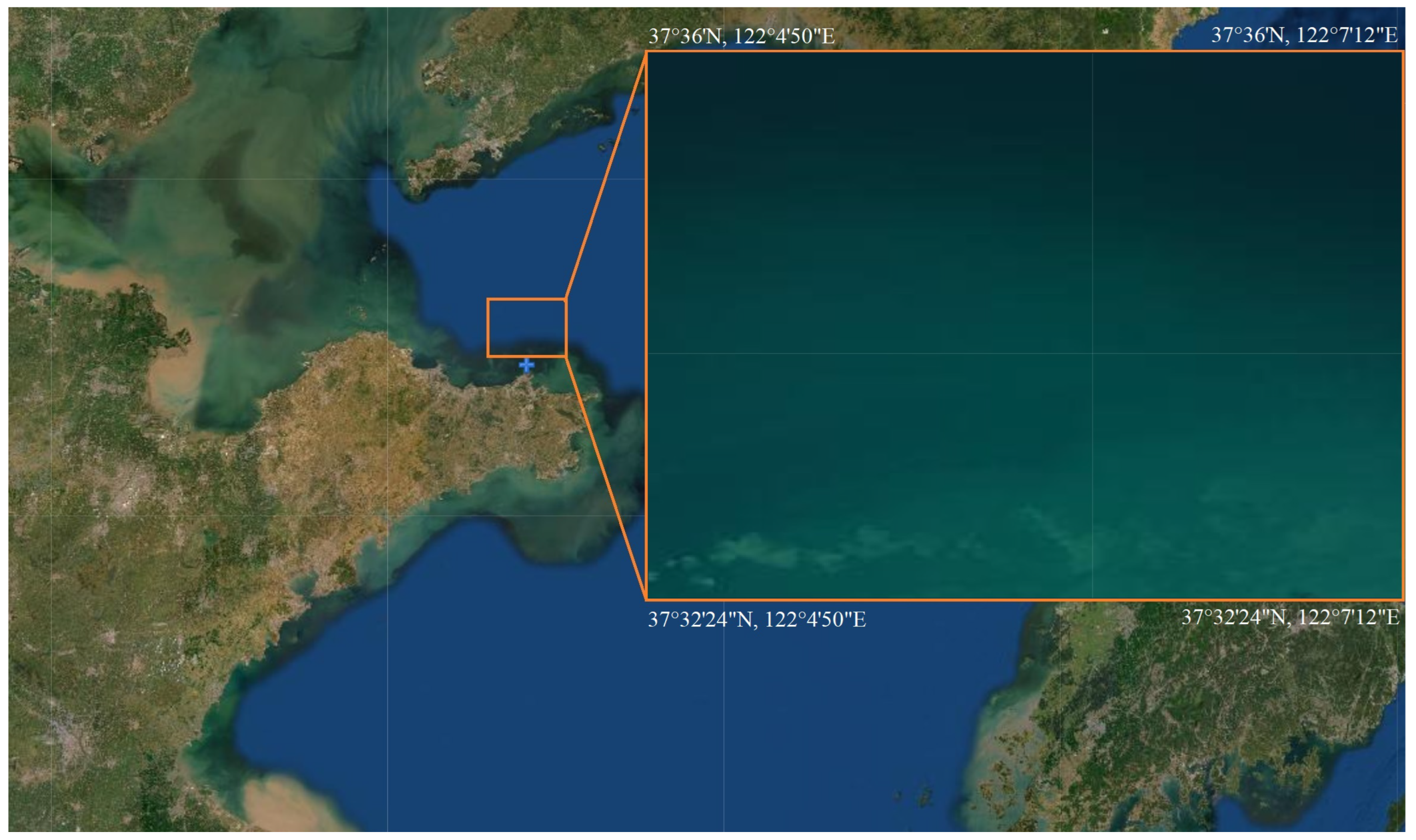
The SSS data were collected in the Yellow Sea waters of China to validate our proposed methods. The surveyed area is presented in Figure 1.

SSS data were acquired using Klein4000 SSS. When working at 100 kHz, it can scan the width of more than 600 m on one side. The images we used are the resolved images of the sonar working at 100 kHz. To ensure that information on seabed sediments can be obtained for the entire area, the area scanned by two adjacent survey lines must overlap by at least 25%. Time variable gain was applied to eliminate the effect of different water depths on SSS imaging. After the sonar data were preprocessed, the SSS images were segmented, screened, and labeled to make the dataset for our experiments.

We also conducted a seabed sediments sampling survey in the areas. In this survey, clam grab samplers were used. They are capable of sampling various surface sediments in different waters and water depths, such as ports and oceans. This technique has been widely used in surface sediments investigation and other fields.

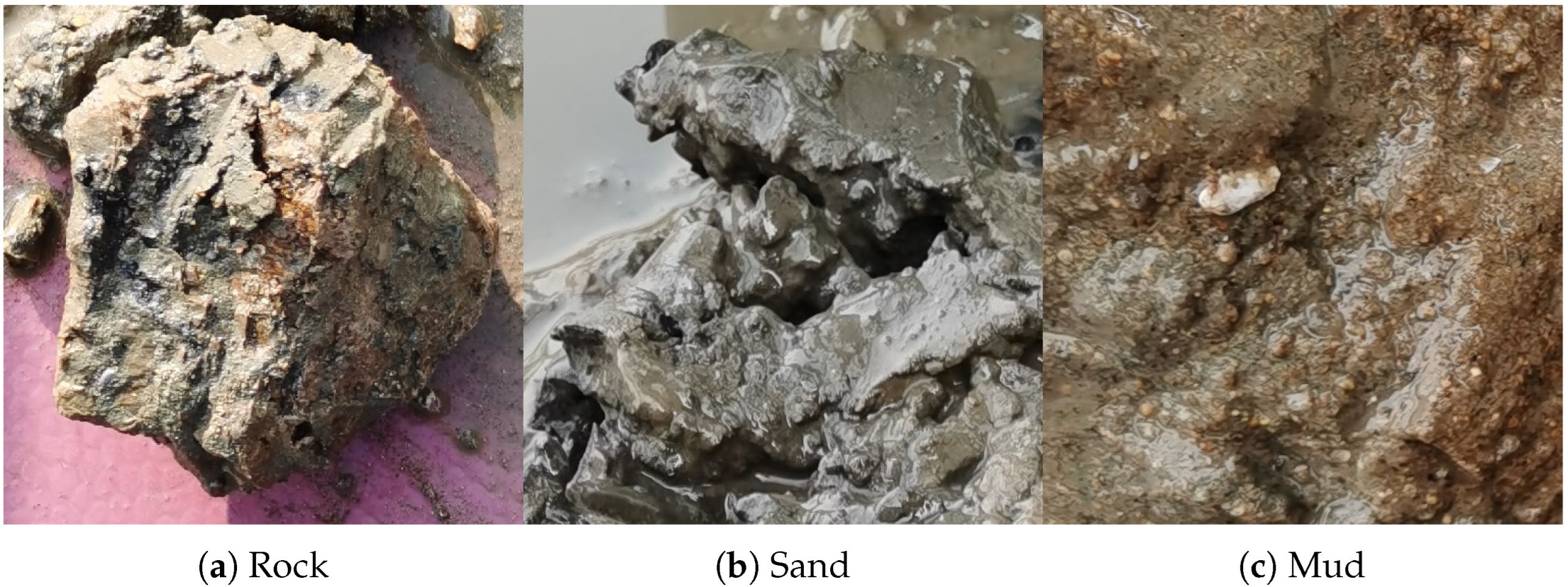
In order to obtain the real distribution of seabed sediments in the survey area, a total of about 500 seabed sediments samples were collected, and the distance between adjacent sediments samples was not more than 200 m. If the collected sample is less than 500 g, we will repeat the grab at the same position. If the total sample mass of five collections at the same location is less than 500 g, we will mark the seabed surface at that location as rocky or an invalid sampling. The collected seabed sediment samples were confirmed to be their type by expert observation and particle size analysis. Figure 2 shows the three types of seabed sediment samples we collected.

2.2. Self-Attention Mechanism

In recent years, the self-attention mechanism has made great breakthroughs in the fields of natural language processing and machine translation [41]. Since the self-attention mechanism has the advantage of being able to focus on significant characteristics and neglect immaterial characteristics, and constantly change the weights in different tasks, self-attention mechanisms have been extensively applied to image classification [42].

The self-attention mechanism is a special attention mechanism that reduces dependence on other knowledge. Compared with the convolutional kernel, it has better performance in identifying the relevance of knowledge. The self-attention mechanism can be defined as a function that maps three vectors of query, key, and value to the output. The output of this function is a weighted sum of values, each weighted by the compatibility of its corresponding query and key. The function of the self-attention mechanism and its output are presented in Equations (1) and (2), respectively:

$$SelfAttention(Q,K,V)=softmax\left(Q{K}^T\right)V$$

(1)

where Q is a tensor concatenated by multiple queries, while K and V are tensors concatenated by multiple key-value pairs, respectively.

$$ou{t}_{SelfAttention}=SelfAttention(Q,K,V)+x$$

(2)

where x is the input of the attention function.

Figure 3 shows the principle and calculation process of the self-attention mechanism.

2.3. SAGAN

It is well known that deep learning is data-driven. In the case of small-samples, many image classifiers can perform poorly in classification. For the same classifier, in most cases, more training data can achieve better classification results. The sonar images of seabed sediments are low-resolution grayscale images, mainly composed of grayscale and sediment texture information. Furthermore, some types of sediment images are visually more like noise, and these sediment images usually do not contain enough feature information as images of human faces or buildings. Therefore, it is necessary to use a large amount of training data to improve the classification accuracy of the model. However, since the acquisition of seabed sediments data is very expensive and difficult, we can only use a small amount of data to build and train a seabed sediment classifier. To solve the above-mentioned issues, SAGAN [40] is used for data augmentation.

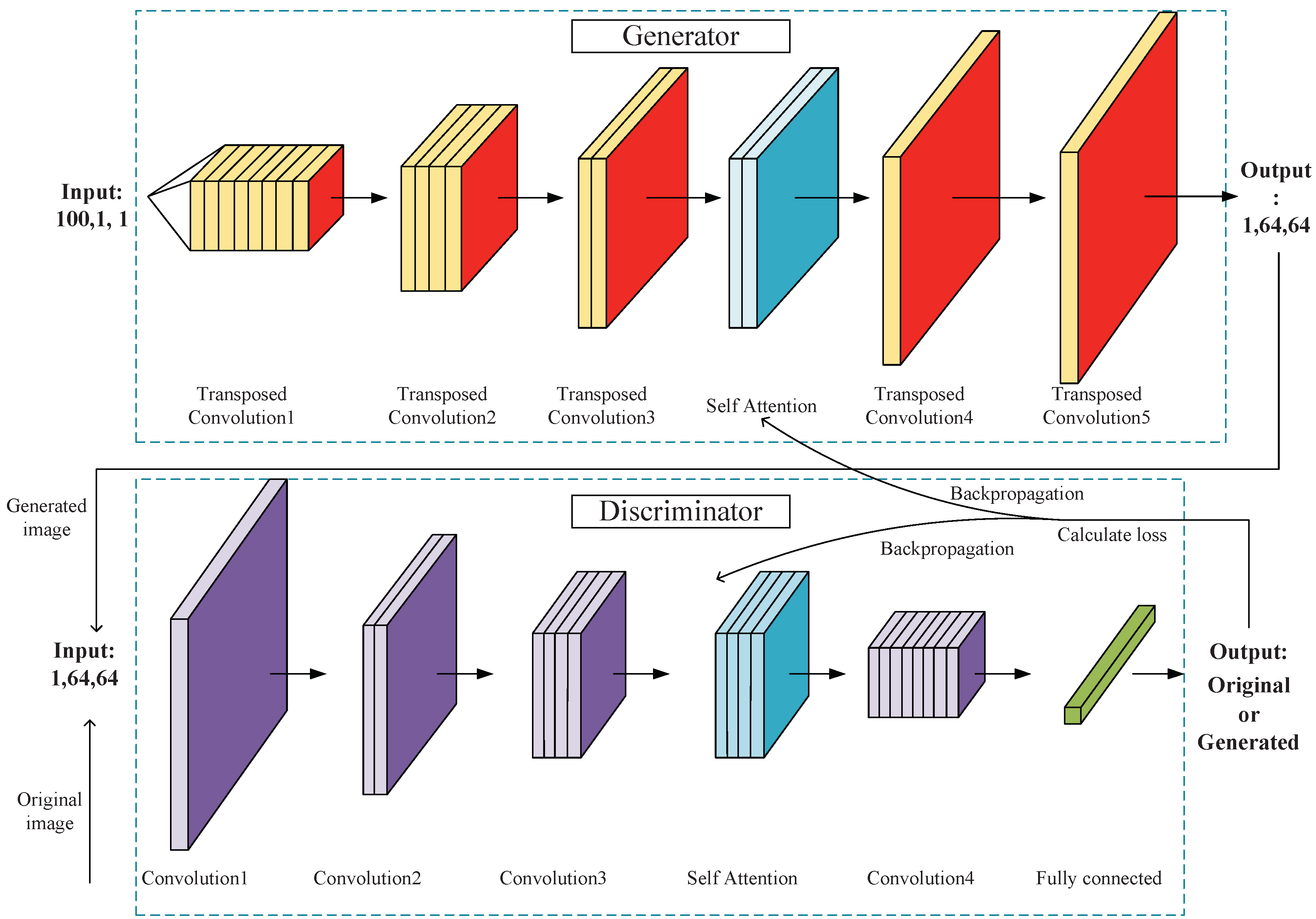
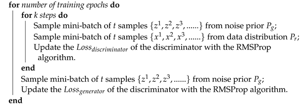
Figure 4 shows the network structure of SAGAN. SAGAN consists of two sub-networks, the generator and the discriminator. The task of the generator is to continuously learn the distribution of data and create fake data to deceive the discriminator. The task of the discriminator is to continuously determine whether the data are real or generated. The two networks co-evolve in a constant game until the discriminator cannot tell whether the data are real or generated by the generator, or until the set number of training epochs is completed. The purpose of this study is to obtain a trained generator for data augmentation to enrich data features and improve the performance of the sediment classifier. The training of SAGAN is detailed in Algorithm 1.

The generator network we adopt contains a total of five transposed convolutional layers and a self-attention layer. The output of every transposed convolutional layer is subjected to the batch normalization (BN) operation [43] to increase the convergence speed of the network. In addition, only the convolutional and self-attention layers were used. The fully-connected layer does not contribute significantly to the quality of the generated images and increases the number of network parameters. Removing the fully connected layer does not reduce the quality of image generation and can improve the parameter adjustment speed of the SAGAN. We did not select spectral normalization in the generator, but we did in the discriminator. Equation (3) shows the loss function:

$$Los{s}_{generator}=-\underset{D\left(G\left(z\right)\right)\sim P_g}{E}\left[D\left(G\left(z\right)\right)\right]$$

(3)

where $P_g$ is the distribution of the generated image, z is the input noise, and $D,G$ are the functions of the generator and discriminator, respectively.

There are several fully connected layers, four convolutional layers and one self-attention layer, in the discriminator network. Likewise, we also minimized the parameters of the fully connected layers to make the network easier to train. The loss function of the discriminator network of Wasserstein generative adversarial network with gradient penalty (WGAN-GP) is widely used due to its good performance [44]. WGAN-GP makes the network satisfy Lipschitz-1 continuity by using a penalty. The loss of the discriminator network of WGAN-GP is shown in Equation (4):

$$Los{s}_{WGAN-GP}=\underset{gradientpenalty}{\underbrace{\lambda E\left[max{\left(0,\left({\parallel {\nabla }_{\widehat{x}}D\left(\widehat{x}\right)-1\parallel }_2\right)\right)}^2\right]}}+\underset{D\left(G\left(z\right)\right)\sim P_g}{E}\left[D\left(G\left(z\right)\right)\right]-\underset{D\left(x\right)\sim P_r}{E}\left[D\left(x\right)\right]$$

(4)

where $P_r$ is the distribution of the real data, x is the original data, $\lambda$ is the penalty coefficient, and $\widehat{x}=G\left(z\right)$.

However, in our network, the spectral normalization [45] was used on the discriminator network to make it satisfy Lipschitz-1 continuity. Therefore, the penalty term in the loss function could be removed. The discriminator function in our network is given in Equation (5):

$$Los{s}_{discriminator}=\underset{D\left(G\left(z\right)\right)\sim P_g}{E}\left[D\left(G\left(z\right)\right)\right]-\underset{D\left(x\right)\sim P_r}{E}\left[D\left(x\right)\right]$$

(5)

Algorithm 1: SAGAN

2.4. SADenseNet

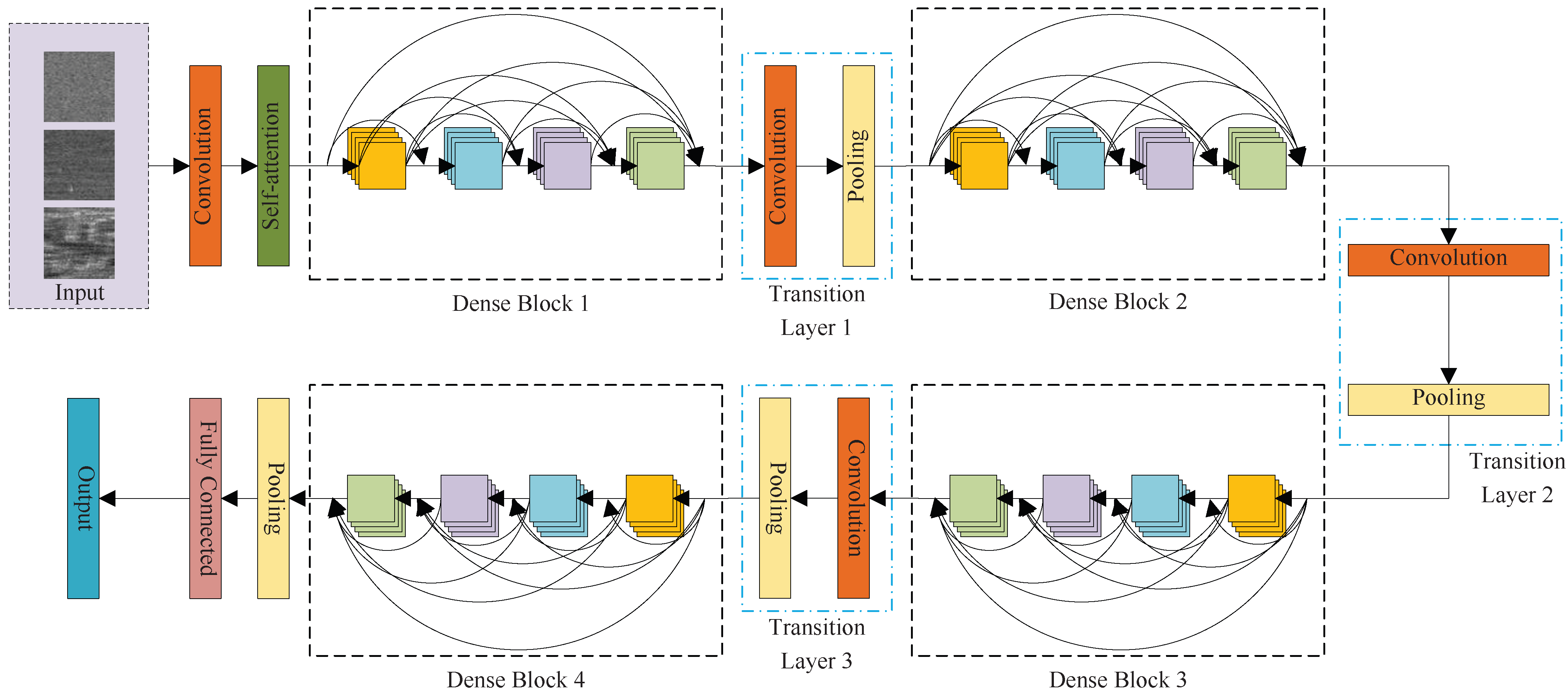
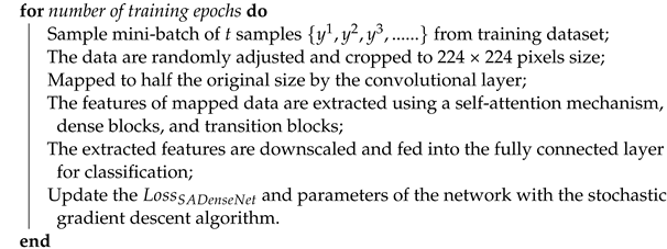
Although many well-performing classification networks have been proposed, the accuracy of seabed sediment classification still needs to be improved. Due to the powerful advantages of the self-attention mechanism (see Section 2.2 for details) and the good classification performance of DenseNet, we introduced the self-attention mechanism into DenseNet, thus proposing SADenseNet to improve the accuracy of seabed sediment classification. The overall structure of SADenseNet containing four dense blocks is shown in Figure 5. The training process of SADenseNet is shown in Algorithm 2.

Dense connectivity has been proposed to better utilize the characteristics of different layers in the network as well as to improve the flow of information between the layers. In ResNet, the output of a layer was derived by summing the input of that layer with its nonlinear transformation. Conversely, in SADenseNet, the output of a layer was determined by all its preceding layers, and the features were combined by concatenation.

$$y_l=H_l\left([y_0,y_1,y_2,...,y_{l-1}]\right)$$

(6)

where $[y_0,y_1,y_2,...,y_{l-1}]$ refers to the concatenation of the feature maps generated at layers $0,1,2,...,l-1$ and $H_l\left(\right)$ is a composite function of BN, rectified linear unit (ReLU), 1 × 1 convolution (Conv), BN, ReLU, and 3 × 3 Conv, in that order.

The number of channels of the output of $H_l\left(\right)$ was $c_0+c(l-1)$, where $c_0$ was the number of channels of the input and l referred to the $lth$ layer of the network. We defined the hyperparameter c as the growth rate of SADenseNet. The channels of each 3 × 3 Conv in the dense block were 32. Before each 3 × 3 Conv, we used BN-ReLU-Conv (1 × 1), which aimed to make the channels of the feature map lower to accelerate the convergence speed of the network and also to fuse the features of each channel. The number of output channels for each 1 × 1 Conv was $4c$.

The transition layer is an important module that connects two dense blocks. It includes 2 × 2 average pooling, 1 × 1 Conv, BN, and ReLU. Here, the role of 1 × 1 Conv is to compress the number of channels of feature maps to half of the input, and the average pooling was used to change the size of each feature map to half of the original, which improve the computational speed and computational efficiency of the network. Moreover, the size of each output feature map was the same as the next dense block.

Global average pooling is the calculation of the average of the features in each channel, reducing their size to 1 × 1. It can scan the global knowledge of each channel and greatly simplify network structure, effectively suppressing network overfitting.

The cross-entropy loss function was used in our proposed network ((7)).

$$Los{s}_{SADenseNet}=-\sum _{j=1}^N{y_r}^j\ast log{{\widehat{y}}_r}^j$$

(7)

where j represents a particular seabed sediment type and N is the number of types of seabed sediments. ${y_r}^j$ is a one-hot vector, indicating that the true sediments type of this sample is type j. ${{\widehat{y}}_r}^j$ means the probability that this sample is predicted to type j.

Algorithm 2: SADenseNet

2.5. Baseline Methods

In order to prove the significance of SADenseNet, many methods, such as SVM [30], KNN [46], RF [3], LeNet [47], AlexNet [48], VGG [49], GoogLeNet [9], ResNet [10], DenseNet [11], Vision Transformer (ViT) [12], and Swin Transformer (SwinT) [50], were selected as baseline methods. These methods have been proven effective in some classification tasks.

3. Experiments and Results

3.1. Original Dataset

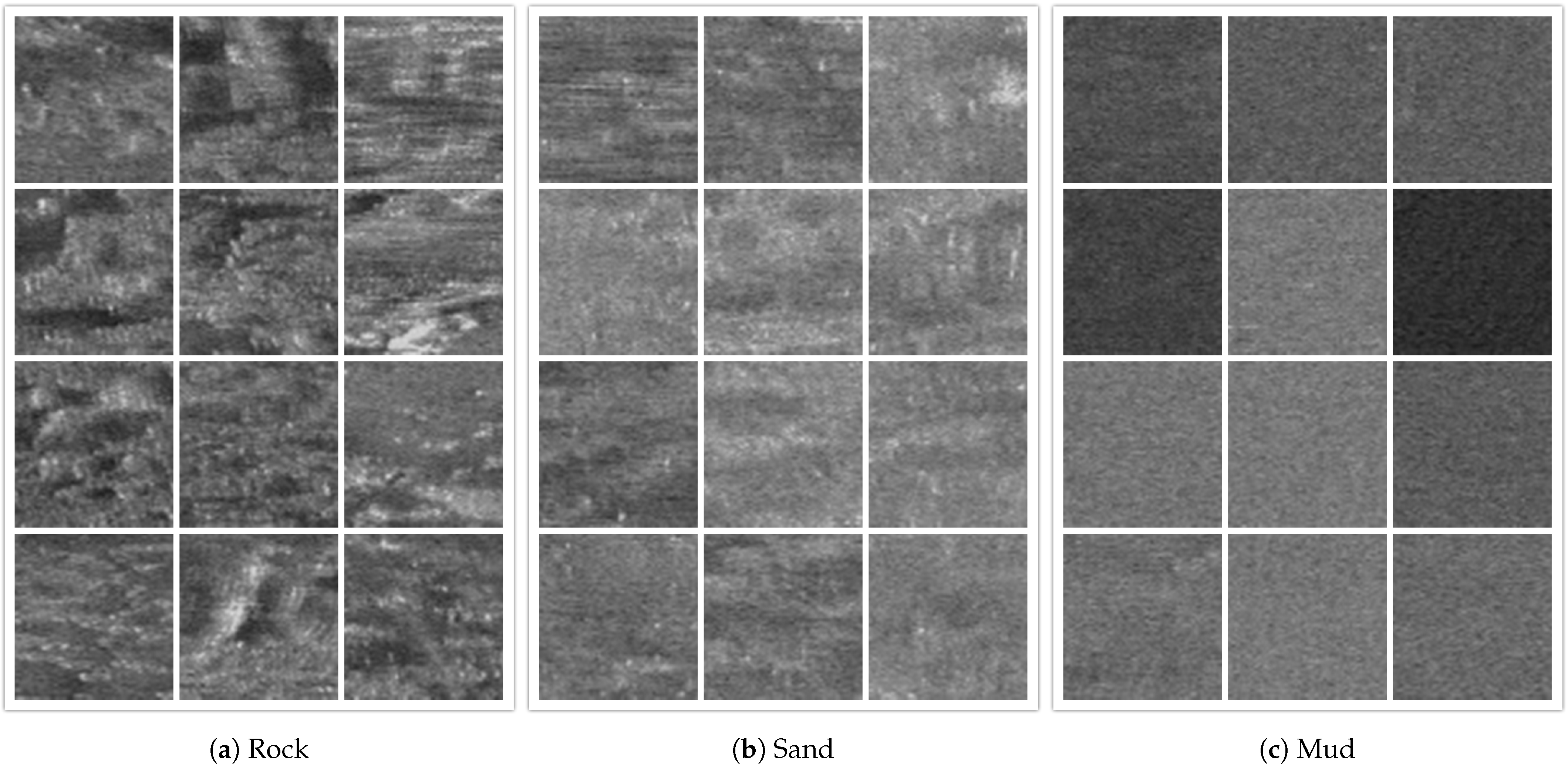
The collected data were preprocessed, segmented, and labeled to create our original dataset, with a total of 686 SSS images. In order to prove the significance of SAGAN and SADenseNet, the amount of data in the training set are far less than that in the test set. There are 110 SSS images in the training set and 576 images in the test set. The size of each image is 64 × 64 pixels. The specific details of the dataset are shown in

Table 1. The original dataset includes 686 samples of mud, rock, and sand.

	Type	Rock	Sand	Mud	Overall
Dataset
Training set		30	50	30	110
Test set		156	187	233	576
Overall		186	237	263	686

, and some SSS images are presented in Figure 6.

3.2. Experimental Setup

Table 2. The structure and parameters of the generator.

			Generator
Layer name	T-Conv1	T-Conv2	T-Conv3	Self-attention	T-Conv4	T-Conv5
Channel	512	256	128	128	64	1
Padding	0	0	0	×	0	0
Kernel size	5	5	5	×	5	4
Stride	2	2	2	×	2	1
Activation	ReLU	ReLU	ReLU	×	ReLU	Sigmoid
Normalization	Batch Norm	Batch Norm	Batch Norm	×	Batch Norm	×

and

Table 3. The structure and parameters of the discriminator.

			Discriminator
Layer name	Conv1	Conv2	Conv3	Self-attention	Conv4	Linear
Channel	64	128	256	256	512	1
Padding	0	0	0	×	0	×
Kernel size	5	5	5	×	5	4
Stride	2	2	2	×	2	1
Activation	ReLU	ReLU	ReLU	×	ReLU	Sigmoid
Normalization	Spectral Norm	Spectral Norm	Spectral Norm	×	Spectral Norm	×

show the network parameters of the generator and discriminator of SAGAN, respectively. The initial learning rate was set to $1\times {10}^{-4}$. The network structure of our proposed SADenseNet is shown in

Table 4. The growth rate of the network is $c=32$, and all “conv” in the table refers to executing BN-ReLU-Conv in order.

Layers	Output Size	Parameters	Output Channels
Convolution	112 × 112	7 × 7 conv, stride = 2	64
Self-attention	112 × 112	$softmax\left(Q{K}^T\right)V+x$	64
Pooling	56 × 56	3 × 3 max pooling, stride = 2	64
Dense Block 1	56 × 56	(1 × 1 conv, 3 × 3 conv) × 6	256
Transition Layer 1-1	56 × 56	1 × 1 conv	128
Transition Layer 1-2	28 × 28	2 × 2 average pooling, stride = 2	128
Dense Block 2	28 × 28	(1 × 1 conv, 3 × 3 conv) × 12	512
Transition Layer 2-1	28 × 28	1 × 1 conv	256
Transition Layer 2-2	14 × 14	2 × 2 average pooling, stride = 2	256
Dense Block 3	14 × 14	(1 × 1 conv, 3 × 3 conv) × 24	1024
Transition Layer 3-1	14 × 14	1 × 1 conv	512
Transition Layer 3-2	7 × 7	2 × 2 average pooling, stride = 2	512
Dense Block 4	7 × 7	(1 × 1 conv, 3 × 3 conv) × 16	1024
Global Average Pool	1 × 1	global average pooling	1024
Fully Connected Layer	1 × 3	fully-connected, softmax	1

. The initial learning rate was set to $1\times {10}^{-3}$.

3.3. Images Augmentation with SAGAN

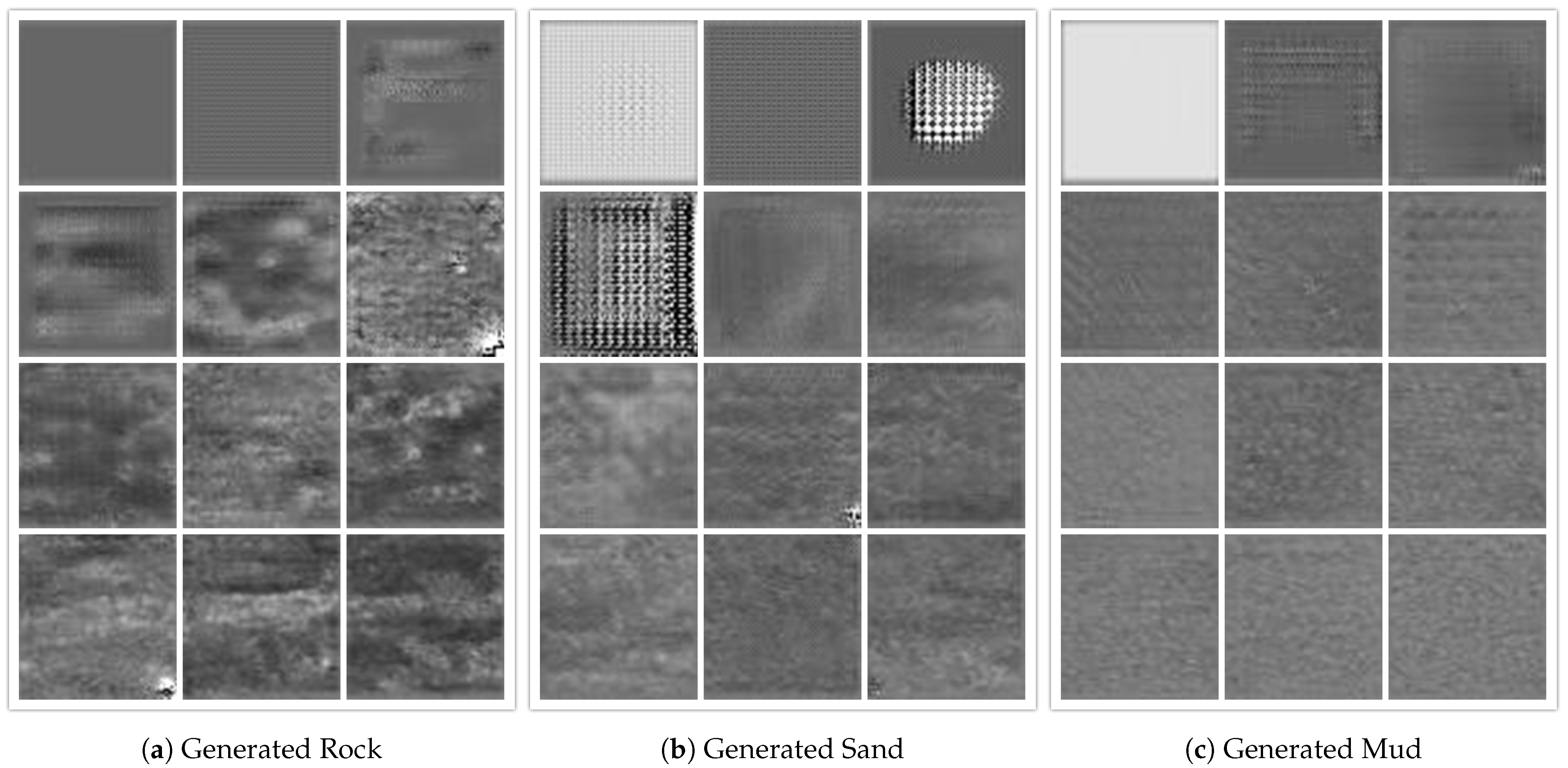
SAGAN was trained for 5000 epochs and the images generated by the network at different epochs are presented in Figure 7. A total of 30,000 images have been generated. The generated images gradually change from fuzzy to clear and from abstract to concrete as the number of training increases in Figure 7. Finally, we manually selected the 880 images generated by SAGAN based on the image visual effects. These images were used to augment the original dataset, and the new dataset is called the augmented dataset.

Table 5. The augmented dataset was also divided into a training set and a test set. The generated sediment images are assigned to the augmented training set, and the test set is the same as the original test set.

	Type	Rock	Sand	Mud	Overall
Dataset
Training set		330	330	330	990
Test set		156	187	233	576
Overall		186	237	263	1566

describes the augmented dataset in detail. Figure 8 shows some of the generated seabed sediment images that were ultimately selected. We did not find the difference between the generated image and the original image by visual observation. To further validate the similarity of the generated images to the original data, the Fréchet Inception Distance (FID) between these generated images and the real images was calculated. FID is a measure of the distance between the feature vectors of the real image and the generated image [51]. The smaller the FID, the more similar the two sets of images are, or the more similar their statistics are. When FID is 0, it indicates that the two sets of images are the same. In addition, 110 real images were selected as the training set and 880 generated images were selected as the test set to verify the effectiveness of SAGAN. The results of these experiments are shown in

Table 6. Classification accuracy and kappa coefficient using the original training set and the generated images as the test set.

	Accuracy	Rock	Sand	Mud	Overall	Kappa
Model
SVM		79.00%	92.14%	98.67%	89.89%	0.848
KNN		86.00%	86.79%	93.67%	88.86%	0.833
RF		81.00%	78.21%	83.00%	80.80%	0.710
LeNet		83.67%	88.57%	95.33%	89.21%	0.838
AlexNet		85.67%	90.00%	99.33%	91.70%	0.876
VGG		81.00%	87.86%	99.00%	89.32%	0.840
ResNet		89.33%	93.93%	92.67%	91.93%	0.879
GoogLeNet		86.00%	93.93%	99.00%	92.96%	0.894
DenseNet		93.00%	86.43%	98.33%	92.73%	0.891
ViT		89.33%	78.57%	83.33%	83.86%	0.758
SwinT		75.00%	91.43%	99.00%	88.41%	0.826
SADenseNet		93.33%	94.64%	99.33%	95.80%	0.937

. The FID of images that have not been manually selected is 60.61, while the FID of images that have been manually selected is 47.29.

3.4. Comparison of Classification Accuracy Using Original SSS Images

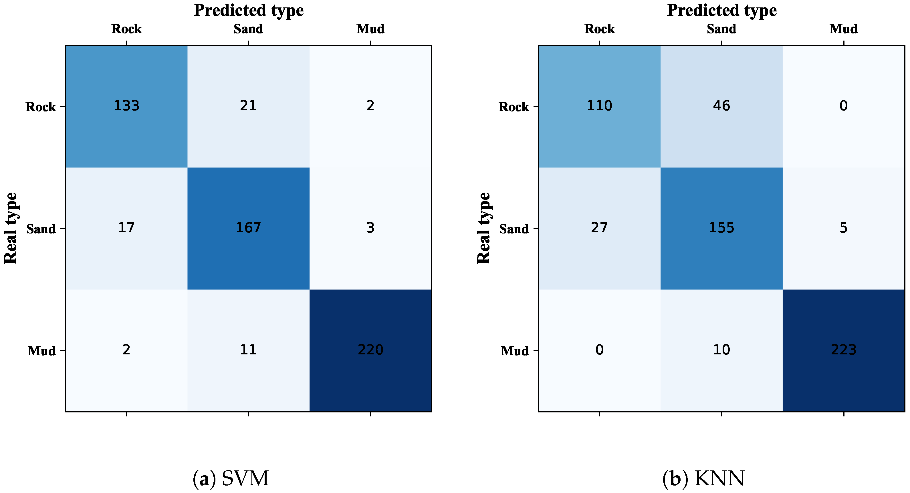
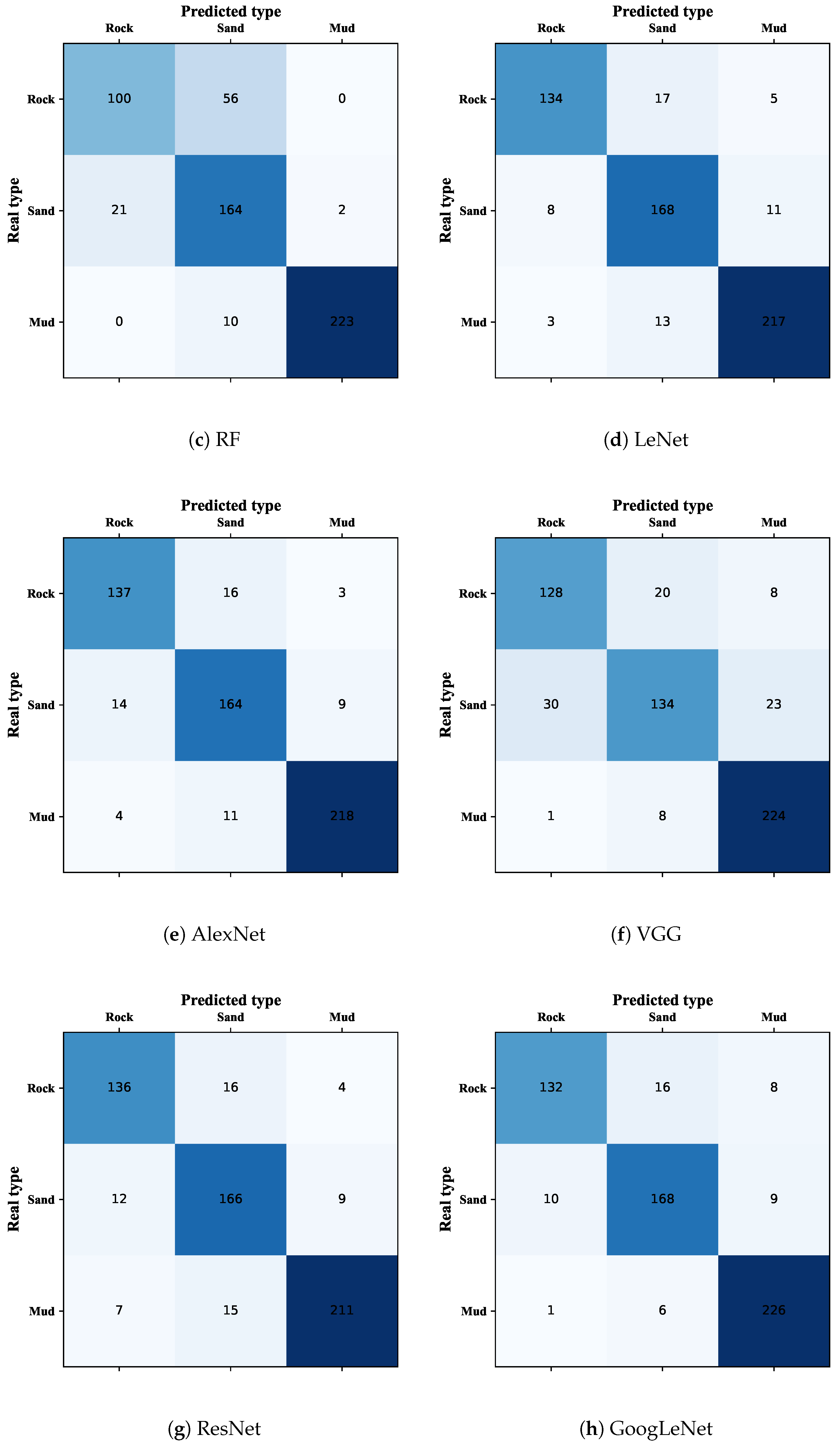
To demonstrate the effectiveness of our proposed SADenseNet, eleven classification methods were selected for comparative analysis, and the number of parameters based on different deep-learning-based classification models is given in

Table 7. Parameters of different classifiers based on deep learning.

Models	LeNet	Alexnet	VGG	GoogLeNet	ResNet	DenseNet	ViT	SwinT	SADenseNet
Parameters	0.6 M	61 M	138 M	7 M	22 M	8 M	86 M	29 M	10 M

. The classification results of the classification methods are detailed in Figure 9 and

Table 8. Classification accuracy and kappa coefficient of different classifiers trained using the original training set.

	Accuracy	Rock	Sand	Mud	Overall	Kappa
Model
SVM		85.26%	89.30%	94.42%	90.28%	0.852
KNN		70.51%	82.89%	95.71%	84.72%	0.767
RF		64.10%	87.70%	95.71%	84.55%	0.764
LeNet		85.90%	89.84%	93.13%	90.10%	0.849
AlexNet		87.82%	87.70%	93.56%	90.10%	0.850
VGG		82.05%	71.66%	96.14%	84.38%	0.761
ResNet		87.18%	88.77%	90.56%	89.06%	0.834
GoogLeNet		84.61%	89.84%	97.00%	91.32%	0.867
DenseNet		90.38%	90.37%	94.85%	92.19%	0.881
ViT		82.05%	71.66%	93.13%	83.16%	0.744
SwinT		83.33%	80.75%	97.00%	88.02%	0.817
SADenseNet		92.31%	91.44%	97.85%	94.27%	0.913

. In Table 8, we can find that SVM, KNN, RF, LeNet, AlexNet, VGG, ResNet, DenseNet, GoogLeNet, SADenseNet, ViT, and SwinT all have good classification performance. Among all the baseline methods, the best classification performance for overall, sand, rock, and mud was 92.19%, 90.37%, 90.38%, and 97.00%, respectively. RF has the worst result for identifying rock, with only 64.10% classification accuracy. KNN and RF do not identify rock very well. The worst performers for sand classification are VGG and ViT, with only 71.66% classification accuracy. The worst performer for mud classification is ResNet, which still has a classification accuracy of 90.56%. All of these 12 models are able to identify mud very well, and specifically, all of them are no less than 90% accurate for the classification of mud. In addition to classification accuracy, we also selected the kappa coefficient as our evaluation index. The kappa coefficient is an indicator used for consistency testing and can also be used to measure the effectiveness of classification [52]. ViT produces the worst overall classification accuracy and the smallest kappa coefficient of 0.744.

Whether it is the identification of any type of sediment, SADenseNet has the best performance. As can be seen from the confusion matrix of each model in Figure 9, these models may identify some of the rock or mud as sand or may identify sand as rock or mud, but will rarely identify rock as mud and vice versa.

3.5. Comparison of Classification Accuracy Using Augmented SSS Images

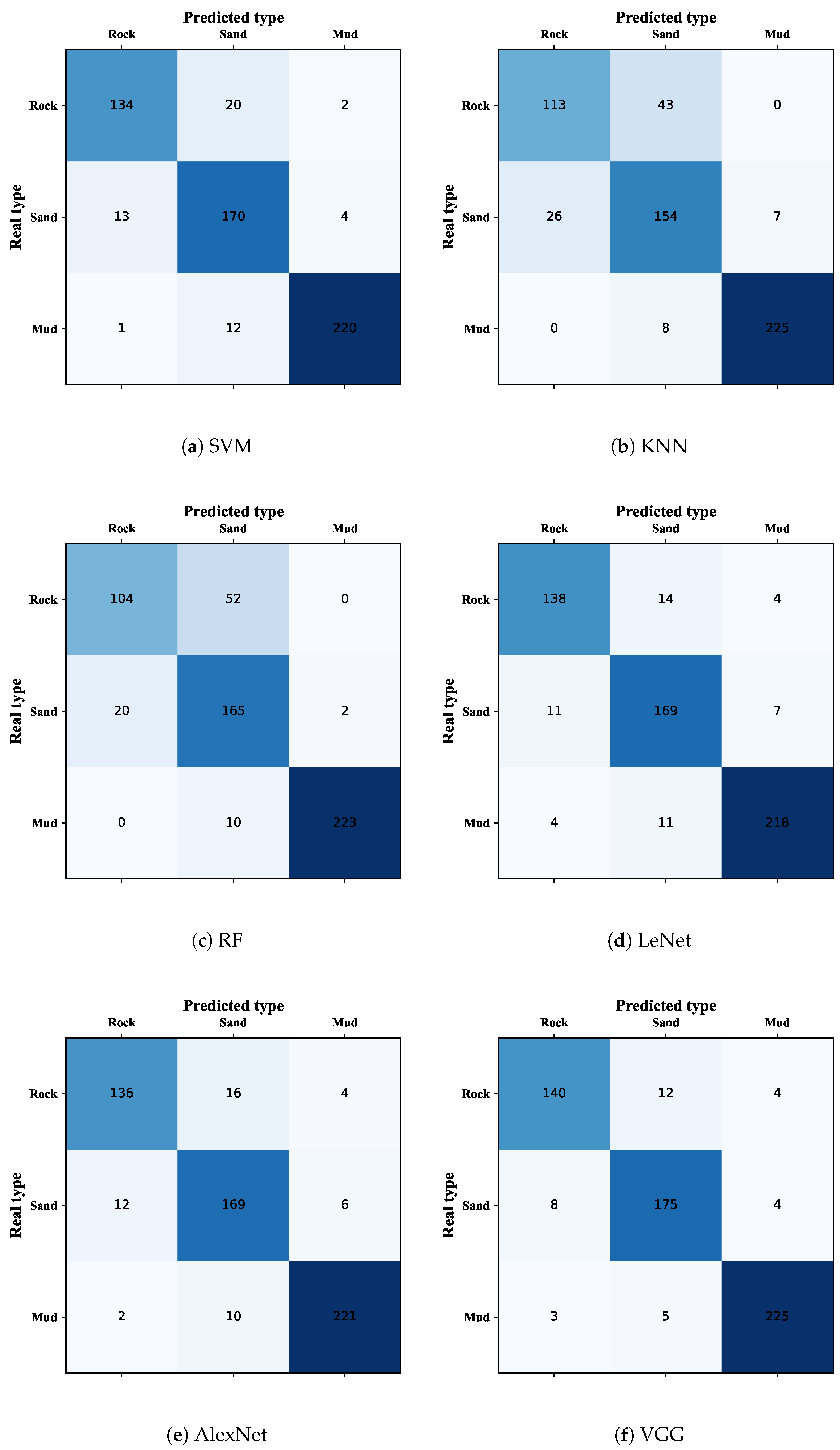
The confusion matrix and classification accuracy of the network trained with the augmented dataset are presented in Figure 10 and

Table 9. Classification accuracy and kappa coefficients of different classifiers trained with the augmented training set. ↑, ↕, and ↓ mean increase, remain the same, and decrease, respectively.

	Accuracy	Rock	Sand	Mud	Overall	Kappa
Model
SVM		85.90% ↑	90.91% ↑	94.42% ↕	90.97% ↑	0.863 ↑
KNN		72.44% ↑	82.35% ↓	96.57% ↑	85.42% ↑	0.778 ↑
RF		66.67% ↑	88.24% ↑	95.71% ↕	85.42% ↑	0.778 ↑
LeNet		88.46% ↑	90.37% ↑	93.56% ↑	91.15% ↑	0.865 ↑
AlexNet		87.18% ↓	90.37% ↑	94.85% ↑	91.39% ↑	0.868 ↑
VGG		89.74% ↑	93.58% ↑	96.57% ↑	93.75% ↑	0.905 ↑
ResNet		89.10% ↑	90.37% ↑	95.71% ↑	92.19% ↑	0.881 ↑
GoogLeNet		89.10% ↑	91.98% ↑	95.71% ↓	92.71% ↑	0.889 ↑
DenseNet		90.38% ↕	92.51% ↑	97.00% ↑	93.75% ↑	0.905 ↑
ViT		84.62% ↑	88.77% ↑	94.85% ↑	90.10% ↑	0.849 ↑
SwinT		86.54% ↑	88.24% ↑	97.85% ↑	91.67% ↑	0.872 ↑
SADenseNet		92.31%↕	95.72%↑	97.85%↕	95.28%↑	0.934↑

, respectively. The best classification performance of the baseline methods for overall, sand, rock, and mud was 93.75%, 93.58%, 90.38%, and 97.85%, respectively. RF performs the worst in identifying rock, with only 66.67% classification accuracy. However, rock and mud are not misclassified by RF. The worst performer for sand classification is KNN, with 82.35% classification accuracy, although rock and mud are not misclassified by KNN, similar to RF. The classifier with the worst ability to identify mud is LeNet, which still has a good performance of 93.56%. In general, KNN and RF have the worst overall classification accuracy of 85.42% and a kappa coefficient of 0.778. In the case of misclassification, rock and sand are misclassified or sand and mud are misclassified, while rock and mud are hardly ever misclassified. Moreover, all the metrics of SADenseNet are the best among these 12 methods.

Compared to using the original dataset, the majority of the overall classification accuracy, kappa coefficient, and classification accuracy of particular sediments were all somewhat improved when we used the augmented dataset to train these 12 classifiers. The average improvement in classification accuracy was 2.25% for rock, 5.12% for sand, 0.97% for mud, 2.64% for overall, and 0.041 for the kappa coefficient. The overall accuracy of the models in order from top to bottom in Table 9 increased by 0.69%, 0.70%, 0.87%, 1.05%, 1.29%, 9.37%, 3.13%, 1.39%, 1.56%, 6.94%, 3.65%, and 1.01%, respectively.

4. Discussion

In seabed sediment classification, to build a classifier with higher classification accuracy and kappa coefficient, there are several approaches, as follows:

(1)

Improving the data quality of seabed sediments by eliminating the influence of the disturbance factors during collection.

(2)

Constructing a better feature extractor.

(3)

Building a better classifier that can better distinguish between different types of seabed sediments.

(4)

Using more data to train the seabed sediment classifier so that the classifier can be trained better.

In this study, we investigate factors (2)–(4) above as follows.

SAGAN is used for data augmentation, which enables SADenseNet to have more training samples to better learn the differences between different types of seabed sediments, thus improving the classification accuracy.

Moreover, a deep-learning-based neural network is constructed called SADenseNet, which can achieve both characteristic construction and classification of seabed sediment images. The self-attention mechanism is introduced in SADenseNet, which can enable the network to better distinguish seabed sediments.

4.1. Image Augmentation

The texture structure presented by SSS images in some sea areas may involve a large spatial range of neighborhoods, and in addition, some classes of images are even close to random distribution. Therefore, in order to better acquire global features of images and generate clear images, larger convolutional kernels as well as deep neural network structures are required. However, such GAN is often difficult to train and obtain satisfactory images. In order to obtain good-quality images, the self-attention mechanism was introduced into the GAN, which is called SAGAN. By adding a self-attention layer to the GAN, the network has a strong global information extraction capability [39]. In order to improve the network’s ability to analyze and generalize global features, both the discriminator and the generator adopt a deep network structure. The addition of the self-attention layer also further enhances the network’s ability to process long-range information, enabling the generated images to reflect the texture patterns of the original images over a larger spatial range [53].

We can see from Figure 7 that as the number of epochs of the network gradually increases, the generated images gradually become concrete from abstract and clear from blurring. Eventually, an image is randomly selected from the selected images, and experts cannot discern whether the image is generated by the generator. The FID of the generated image to the real image is 47.29, which is a good result compared to many advanced GANs [54]. Furthermore, the images that have been manually selected have a smaller FID than those that have not been manually selected. In addition, the classification results using generated images are very similar to using real images as the test set. All these can prove the effectiveness of SAGAN. We divide the generated images into the training set to increase the feature richness of the dataset, and thus, improve the final classification performance of the classifier. Although theoretically, it can have the ability to optimize the processing of seabed sediments data, experiments are still needed to demonstrate its effectiveness. We will describe and analyze the effectiveness of this method in Section 4.3.

4.2. Classification Accuracy Using Original SSS Images

We can see from the data in Table 8 that the traditional machine learning methods have good classification results, especially SVM, which has better performance than many deep-learning-based classification models. Deep-learning-based classification models are data-driven, and a large amount of training data is required to make these networks learn the characteristics of different types of sediments adequately. Furthermore, the training samples for this set of experiments were small, so a portion of the deep-learning-based classification models performed worse than traditional machine models. In contrast, SVM requires only a small amount of data to determine the segmentation hyperplane, so it will also have good performance under small-sample conditions. ViT has the worst performance. The number of parameters for the deep learning model is given in Table 7. Compared to other deep-learning-based classification models, ViT is a very large model, which means that more data are needed to train it to achieve satisfactory performance. Our training set is a very small dataset, which makes it difficult to train ViT adequately. Furthermore, the data dependence of ViT is much greater compared to convolutional neural networks of various structures. GoogLeNet and DenseNet introduce the inception module and dense connection, respectively. Inception module concatenates feature maps of different sizes, and dense connection improves feature flow between layers and enhances feature reuse. Inception module and dense connectivity reduce the data dependency of the network to some extent. In small-sample data classification tasks, a network with an inception module or dense connection will have better classification performance and kappa coefficients compared to a network without inception modules or dense connection.

The proposed SADenseNet has higher accuracy of sediment classification and larger kappa coefficients compared with the state-of-the-art models. The self-attention mechanism is introduced into the proposed SADenseNet. With the current development of deep learning technology, the feature extraction ability of deep networks is becoming more and more powerful, which inevitably causes a large amount of feature redundancy while improving network performance. The self-attention is similar to human vision, which can automatically distinguish important information from global information, reduce the interference of unimportant information, and reduce the waste of computational resources caused by some redundant features. In addition, the self-attention mechanism can better acquire the global features of images and improve the classification performance of the network. The proposed SADenseNet also introduces dense connectivity. The dense connectivity improves the information flow between layers, with each layer obtaining input from all previous layers and passing its output to each subsequent layer, which greatly enhances feature reuse and thus improves the performance of the network. Moreover, each layer of the network is designed to be narrow, which also reduces the number of parameters of the network, decreases the computational cost, and makes the network easier to be trained.

As can be seen from the confusion matrix of each classification model in Figure 9, the models rarely identify rock as mud or identify mud as rock. This is because there is a large difference in the physical grain size as well as the texture characteristics between rock and mud. Sand with a larger grain size will have more similar features to rock, which will cause the models to misclassify rock and sand. Similarly, sand with a smaller grain size has similar characteristics to mud, which will also cause misclassification of the model.

4.3. Classification Accuracy Using Augmented SSS Images

Figure 10 and Table 9 show the classification performance of all models, and we can see that the proposed SADenseNet also has the best performance. Meanwhile, the models basically do not misidentify rock and mud with each other. Most of the misidentifications consist of identifying rock or mud as sand or sand as rock or mud, which is consistent with the results using the original dataset.

By analyzing the performance of the classification models listed in Table 8 and Table 9, it can be seen that only very few of the classification accuracy decreased slightly or remained the same, and the vast majority of the classification accuracy, as well as all kappa coefficients, increased. Artificial intelligence algorithms are data-driven; SAGAN was used for data augmentation, which produced more information not available in the original dataset and enriched the number of features in the data. This allows the classification models to be better trained and more accurately map the acoustic images to the correct sediments type. The model with the largest improvement compared to the original training set was VGG, which improved the overall accuracy by 9.37% and the kappa coefficient by 0.144. VGG has the largest number of parameters in these networks (Table 6) and is more data-dependent, so VGG trained with the augmented training set had the largest improvement in performance. These experimental results demonstrate that data augmentation of the training set using SAGAN can indeed improve the performance of the classification model.

Training each classification model with the augmented dataset, the deep-learning-based classification models performed better than the traditional machine learning-based ones, which can also indicate that deep-learning-based classification models can better fit the function that maps sediment images to sediments types when the dataset is larger.

5. Conclusions

In this study, SAGAN is used to learn the data distribution of the original dataset and generate new SSS images to perform data augmentation on the original dataset. Through our experiments, We demonstrate that the images generated by SAGAN are very similar to real images and can augment the features of the original dataset, enabling the classification model to better learn the mapping of SSS images to real sediments types, and the classification model has higher classification accuracy and kappa coefficients.

The self-attention mechanism is introduced into the proposed SADenseNet. The self-attention mechanism can automatically scan the SSS images to obtain the key information of the images and highlight the key features of the images, which can reduce the waste of computational resources caused by feature redundancy. Besides, the self-attention mechanism can also better capture the correlation of the internal information and global features of the images, which contributes to raising the performance of SADenseNet. Dense connectivity is also used in SADenseNet. Dense connectivity enhances feature propagation and feature reuse. The output of each layer will be the input of all the subsequent layers so that the input of each layer is jointly determined by all the preceding layers, which can alleviate the gradient disappearance of the network and improve the classification performance. The transition layer reduces the size of the feature map, which improves the computational efficiency of the network.

The data augmentation method, SAGAN, can also be transferred to other data-starved tasks, and SADenseNet can be extended to challenging tasks, such as underwater target recognition. However, our proposed methods have several limitations, as follows: (1) The quality of data generated by SAGAN is unstable and requires manual selection; (2) SAGAN was trained for more than 30 days in order to generate visually appealing images of seabed sediments, which consumed a large amount of computational resources; (3) In order to make our proposed SADenseNet achieve good classification results, it took about 20 days on parameter tuning, which is time-consuming.

In our future research, we will investigate designing a less computationally expensive and more stable data generator, and build a classifier with a relatively simple structure and better classification performance. In addition, image super-resolution reconstruction technology can effectively solve the problem of low resolution of sonar images, which will be the focus of our research in the future.

References

1. Zhao, J.; Yan, J.; Zhang, H.; Meng, J. A new radiometric correction method for side-scan sonar images in consideration of seabed sediment variation. Remote Sens. 2017, 9, 575. [Google Scholar] [CrossRef]
2. Zhu, Z.; Cui, X.; Zhang, K.; Ai, B.; Shi, B.; Yang, F. DNN-based seabed classification using differently weighted MBES multifeatures. Mar. Geol. 2021, 438, 106519. [Google Scholar] [CrossRef]
3. Zhao, T.; Montereale Gavazzi, G.; Lazendić, S.; Zhao, Y.; Pižurica, A. Acoustic Seafloor Classification Using the Weyl Transform of Multibeam Echosounder Backscatter Mosaic. Remote Sens. 2021, 13, 1760. [Google Scholar] [CrossRef]
4. Zhang, K.; Li, Q.; Zhu, H.; Yang, F.; Wu, Z. Acoustic deep-sea seafloor characterization accounting for heterogeneity effect. IEEE Trans. Geosci. Remote Sens. 2019, 58, 3034–3042. [Google Scholar] [CrossRef]
5. Qin, X.; Luo, X.; Wu, Z.; Shang, J. Optimizing the sediment classification of small side-scan sonar images based on deep learning. IEEE Access 2021, 9, 29416–29428. [Google Scholar] [CrossRef]
6. Li, M.; Tao, Q.; Hou, G.; Zhai, J. A Novel Sub-Bottom Profiler Seabed Sediment Classification Method Based on BPNN With Biot-Stoll Model and Attenuation-Based Model. IEEE Access 2021, 9, 53379–53391. [Google Scholar] [CrossRef]
7. Ji, X.; Yang, B.; Tang, Q. Acoustic seabed classification based on multibeam echosounder backscatter data using the PSO-BP-AdaBoost algorithm: A case study from jiaozhou bay, China. IEEE J. Ocean. Eng. 2020, 46, 509–519. [Google Scholar] [CrossRef]
8. Anderson, J.T.; Van Holliday, D.; Kloser, R.; Reid, D.G.; Simard, Y. Acoustic seabed classification: Current practice and future directions. ICES J. Mar. Sci. 2008, 65, 1004–1011. [Google Scholar] [CrossRef]
9. Szegedy, C.; Liu, W.; Jia, Y.; Sermanet, P.; Reed, S.; Anguelov, D.; Erhan, D.; Vanhoucke, V.; Rabinovich, A. Going deeper with convolutions. In Proceedings of the IEEE Conference on Computer Vision and Pattern Recognition, Boston, MA, USA, 7–12 June 2015; pp. 1–9. [Google Scholar] [CrossRef]
10. He, K.; Zhang, X.; Ren, S.; Sun, J. Deep residual learning for image recognition. In Proceedings of the IEEE Conference on Computer Vision and Pattern Recognition, Las Vegas, NV, USA, 26 June–1 July 2016; pp. 770–778. [Google Scholar] [CrossRef]
11. Huang, G.; Liu, Z.; Van Der Maaten, L.; Weinberger, K.Q. Densely connected convolutional networks. In Proceedings of the IEEE Conference on Computer Vision and Pattern Recognition, Honolulu, HI, USA, 21–26 July 2017; pp. 4700–4708. [Google Scholar] [CrossRef]
12. Dosovitskiy, A.; Beyer, L.; Kolesnikov, A.; Weissenborn, D.; Zhai, X.; Unterthiner, T.; Dehghani, M.; Minderer, M.; Heigold, G.; Gelly, S.; et al. An image is worth 16x16 words: Transformers for image recognition at scale. arXiv 2020, arXiv:2010.11929. [Google Scholar] [CrossRef]
13. Ding, Y.; Zhao, X.; Zhang, Z.; Cai, W.; Yang, N.; Zhan, Y. Semi-supervised locality preserving dense graph neural network with ARMA filters and context-aware learning for hyperspectral image classification. IEEE Trans. Geosci. Remote Sens. 2021, 60, 5511812. [Google Scholar] [CrossRef]
14. Ding, Y.; Zhang, Z.; Zhao, X.; Hong, D.; Cai, W.; Yu, C.; Yang, N.; Cai, W. Multi-feature fusion: Graph neural network and CNN combining for hyperspectral image classification. Neurocomputing 2022, 501, 246–257. [Google Scholar] [CrossRef]
15. Forman, D.J.; Neilsen, T.B.; Van Komen, D.F.; Knobles, D.P. Validating deep learning seabed classification via acoustic similarity. JASA Express Lett. 2021, 1, 040802. [Google Scholar] [CrossRef]
16. Lohse, J.; Doulgeris, A.P.; Dierking, W. An optimal decision-tree design strategy and its application to sea ice classification from SAR imagery. Remote Sens. 2019, 11, 1574. [Google Scholar] [CrossRef]
17. Sales, M.H.; De Bruin, S.; Souza, C.; Herold, M. Land use and land cover area estimates from class membership probability of a random forest classification. IEEE Trans. Geosci. Remote Sens. 2021, 60, 4402711. [Google Scholar] [CrossRef]
18. Koda, S.; Zeggada, A.; Melgani, F.; Nishii, R. Spatial and structured SVM for multilabel image classification. IEEE Trans. Geosci. Remote Sens. 2018, 56, 5948–5960. [Google Scholar] [CrossRef]
19. Chen, L.; Li, S.; Bai, Q.; Yang, J.; Jiang, S.; Miao, Y. Review of image classification algorithms based on convolutional neural networks. Remote Sens. 2021, 13, 4712. [Google Scholar] [CrossRef]
20. Cui, X.; Liu, H.; Fan, M.; Ai, B.; Ma, D.; Yang, F. Seafloor habitat mapping using multibeam bathymetric and backscatter intensity multi-features SVM classification framework. Appl. Acoust. 2021, 174, 107728. [Google Scholar] [CrossRef]
21. Yu, X.; Zhai, J.; Zou, B.; Shao, Q.; Hou, G. A Novel Acoustic Sediment Classification Method Based on the K-Mdoids Algorithm Using Multibeam Echosounder Backscatter Intensity. J. Mar. Sci. Eng. 2021, 9, 508. [Google Scholar] [CrossRef]
22. Gaida, T.C.; Tengku Ali, T.A.; Snellen, M.; Amiri-Simkooei, A.; Van Dijk, T.A.; Simons, D.G. A multispectral Bayesian classification method for increased acoustic discrimination of seabed sediments using multi-frequency multibeam backscatter data. Geosciences 2018, 8, 455. [Google Scholar] [CrossRef]
23. Yan, P.; Feng, X.; Yue, L.J.Z. Seabed Sediment Classification based on Multi-features Fusion and Feature Selection Framework. In Proceedings of the 2021 OES China Ocean Acoustics (COA), Harbin, China, 14–17 July 2021; pp. 378–381. [Google Scholar] [CrossRef]
24. He, L.; Zhao, J.; Lu, J.; Qiu, Z. High-accuracy acoustic sediment classification using sub-bottom profile data. Estuar. Coast. Shelf Sci. 2022, 265, 107701. [Google Scholar] [CrossRef]
25. Li, S.; Zhao, J.; Zhang, H.; Qu, S. Sub-Bottom Sediment Classification Using Reliable Instantaneous Frequency Calculation and Relaxation Time Estimation. Remote Sens. 2021, 13, 4809. [Google Scholar] [CrossRef]
26. Zheng, H.B.; Yan, P.; Chen, J.; Wang, Y.L. Seabed sediment classification in the northern South China Sea using inversion method. Appl. Ocean Res. 2013, 39, 131–136. [Google Scholar] [CrossRef]
27. Wang, F.; Yu, J.; Liu, Z.; Kong, M.; Wu, Y. Study on offshore seabed sediment classification based on particle size parameters using XGBoost algorithm. Comput. Geosci. 2021, 149, 104713. [Google Scholar] [CrossRef]
28. Manik, H.; Albab, A. Side-scan sonar image processing: Seabed classification based on acoustic backscattering. IOP Conf. Ser. Earth Environ. Sci. 2021, 944, 012001. [Google Scholar] [CrossRef]
29. Febriawan, H.; Helmholz, P.; Parnum, I. Support vector machine and decision tree based classification of side-scan sonar mosaics using textural features. Int. Arch. Photogramm. Remote Sens. Spat. Inf. Sci.-ISPRS Arch. 2019, 42, 27–34. [Google Scholar] [CrossRef]
30. Annalakshmi, G.; Murugan, S.S.; Ramasundaram, K. Side Scan Sonar Images Based Ocean Bottom Sediment Classification. In Proceedings of the 2019 International Symposium on Ocean Technology (SYMPOL), Ernakulam, India, 11–13 December 2019; pp. 138–144. [Google Scholar] [CrossRef]
31. Berthold, T.; Leichter, A.; Rosenhahn, B.; Berkhahn, V.; Valerius, J. Seabed sediment classification of side-scan sonar data using convolutional neural networks. In Proceedings of the 2017 IEEE Symposium Series on Computational Intelligence (SSCI), Honolulu, HI, USA, 27 November–1 December 2017; pp. 1–8. [Google Scholar] [CrossRef]
32. Xi, H.; Wan, L.; Sheng, M.; Li, Y.; Liu, T. The study of the seabed side-scan acoustic images recognition using BP neural network. In Proceedings of the Parallel Architecture, Algorithm and Programming: 8th International Symposium, Haikou, China, 17–18 June 2017; pp. 130–141. [Google Scholar] [CrossRef]
33. Yu, Y.; Zhao, J.; Gong, Q.; Huang, C.; Zheng, G.; Ma, J. Real-time underwater maritime object detection in side-scan sonar images based on transformer-YOLOv5. Remote Sens. 2021, 13, 3555. [Google Scholar] [CrossRef]
34. Atallah, L.; Shang, C.; Bates, R. Object detection at different resolution in archaeological side-scan sonar images. In Proceedings of the Europe Oceans 2005, Brest, France, 20–23 June 2005; Volume 1, pp. 287–292. [Google Scholar] [CrossRef]
35. Yulin, T.; Jin, S.; Bian, G.; Zhang, Y. Shipwreck target recognition in side-scan sonar images by improved YOLOv3 model based on transfer learning. IEEE Access 2020, 8, 173450–173460. [Google Scholar] [CrossRef]
36. Hou, S.; Jiao, D.; Dong, B.; Wang, H.; Wu, G. Underwater inspection of bridge substructures using sonar and deep convolutional network. Adv. Eng. Inform. 2022, 52, 101545. [Google Scholar] [CrossRef]
37. Shorten, C.; Khoshgoftaar, T.M. A survey on image data augmentation for deep learning. J. Big Data 2019, 6, 60. [Google Scholar] [CrossRef]
38. Bayer, M.; Kaufhold, M.A.; Reuter, C. A survey on data augmentation for text classification. ACM Comput. Surv. 2022, 55, 1–39. [Google Scholar] [CrossRef]
39. Goodfellow, I.; Pouget-Abadie, J.; Mirza, M.; Xu, B.; Warde-Farley, D.; Ozair, S.; Courville, A.; Bengio, Y. Generative adversarial networks. Commun. ACM 2020, 63, 139–144. [Google Scholar] [CrossRef]
40. Zhang, H.; Goodfellow, I.; Metaxas, D.; Odena, A. Self-attention generative adversarial networks. In Proceedings of the International Conference on Machine Learning, Long Beach, CA, USA, 9–15 June 2019; pp. 7354–7363. [Google Scholar] [CrossRef]
41. Zhao, H.; Jia, J.; Koltun, V. Exploring self-attention for image recognition. In Proceedings of the IEEE/CVF Conference on Computer Vision and Pattern Recognition, Seattle, WA, USA, 14–19 June 2020; pp. 10076–10085. [Google Scholar] [CrossRef]
42. Niu, Z.; Zhong, G.; Yu, H. A review on the attention mechanism of deep learning. Neurocomputing 2021, 452, 48–62. [Google Scholar] [CrossRef]
43. Ioffe, S.; Szegedy, C. Batch normalization: Accelerating deep network training by reducing internal covariate shift. In Proceedings of the International Conference on Machine Learning, Lille, France, 6–11 July 2015; pp. 448–456. [Google Scholar] [CrossRef]
44. Gulrajani, I.; Ahmed, F.; Arjovsky, M.; Dumoulin, V.; Courville, A.C. Improved training of wasserstein gans. Adv. Neural Inf. Process. Syst. 2017, 30. [Google Scholar] [CrossRef]
45. Miyato, T.; Kataoka, T.; Koyama, M.; Yoshida, Y. Spectral normalization for generative adversarial networks. arXiv 2018, arXiv:1802.05957. [Google Scholar] [CrossRef]
46. Ma, L.; Crawford, M.M.; Tian, J. Local manifold learning-based k-nearest-neighbor for hyperspectral image classification. IEEE Trans. Geosci. Remote Sens. 2010, 48, 4099–4109. [Google Scholar] [CrossRef]
47. Kayed, M.; Anter, A.; Mohamed, H. Classification of garments from fashion MNIST dataset using CNN LeNet-5 architecture. In Proceedings of the 2020 International Conference on Innovative Trends in Communication and Computer Engineering (ITCE), Aswan, Egypt, 8–9 February 2020; pp. 238–243. [Google Scholar] [CrossRef]
48. Krizhevsky, A.; Sutskever, I.; Hinton, G.E. Imagenet classification with deep convolutional neural networks. Commun. ACM 2017, 60, 84–90. [Google Scholar] [CrossRef]
49. Simonyan, K.; Zisserman, A. Very deep convolutional networks for large-scale image recognition. arXiv 2014, arXiv:1409.1556. [Google Scholar] [CrossRef]
50. Liu, Z.; Lin, Y.; Cao, Y.; Hu, H.; Wei, Y.; Zhang, Z.; Lin, S.; Guo, B. Swin transformer: Hierarchical vision transformer using shifted windows. In Proceedings of the IEEE/CVF International Conference on Computer Vision, Montreal, BC, Canada, 11–17 October 2021; pp. 10012–10022. [Google Scholar] [CrossRef]
51. Heusel, M.; Ramsauer, H.; Unterthiner, T.; Nessler, B.; Hochreiter, S. Gans trained by a two time-scale update rule converge to a local nash equilibrium. Adv. Neural Inf. Process. Syst. 2017, 30, 6627–6638. [Google Scholar] [CrossRef]
52. Foody, G.M. Thematic map comparison: Evaluating the statistical significance of differences in classification accuracy. Photogramm. Eng. Remote Sens. 2004, 70, 627–634. [Google Scholar] [CrossRef]
53. Vaswani, A.; Shazeer, N.; Parmar, N.; Uszkoreit, J.; Jones, L.; Gomez, A.N.; Kaiser, Ł.; Polosukhin, I. Attention is all you need. Adv. Neural Inf. Process. Syst. 2017, 30. [Google Scholar] [CrossRef]
54. Wei, J.; Liu, M.; Luo, J.; Zhu, A.; Davis, J.; Liu, Y. DuelGAN: A Duel between Two Discriminators Stabilizes the GAN Training. In Proceedings of the European Conference on Computer Vision, Tel Aviv, Israel, 23–27 October 2022; pp. 290–317. [Google Scholar] [CrossRef]
Figure 1. The area of data collection is situated in the northern part of Weihai City, Shandong Province, China. The area is approximately 20 square kilometers. In this area, a total of three types of sediment were collected, namely rock, sand, and mud.
Remotesensing 15 02178 g001
Figure 2. The three types of seabed sediment samples we collected in the investigation.
Remotesensing 15 02178 g002
Figure 3. The data processing flow of the self-attention mechanism.
Remotesensing 15 02178 g003
Figure 4. The overall structure and calculation process of SAGAN. The input of SAGAN is a 100 × 1 × 1 tensor of noise and the output is a 64 × 64 gray-scale image.
Remotesensing 15 02178 g004
Figure 5. The proposed SADenseNet has four dense blocks. There is a transition layer between adjacent dense blocks, which reduces the dimensionality of the features and makes them uniform in size, which greatly improves computational efficiency.
Remotesensing 15 02178 g005
Figure 6. Three types of original SSS images of seabed sediments.
Remotesensing 15 02178 g006
Figure 7. From left to right, from top to bottom, the different types of seabed sediment images generated by SAGAN are shown in turn with the increasing number of epochs. As the epochs increases, the three types of seabed sediment images generated by SAGAN gradually change from fuzzy and abstract to clear and concrete.
Remotesensing 15 02178 g007
Figure 8. The filtered generated seabed sediment images.
Remotesensing 15 02178 g008
Figure 9. Confusion matrices of different classifiers trained with the original dataset.
Remotesensing 15 02178 g009aRemotesensing 15 02178 g009bRemotesensing 15 02178 g009c
Figure 10. Confusion matrices of different classifiers trained with the augmented dataset.
Remotesensing 15 02178 g010aRemotesensing 15 02178 g010b