Abstract
Earthquakes are a severe natural phenomenon that require continuous monitoring, analysis, and forecasting to mitigate their risks. Seismological data have long been used for this purpose, but geodynamic data from remote sensing of surface displacements have become available in recent decades. In this paper, we present a novel information technology for monitoring, analyzing seismogenic fields, and predicting earthquakes using Earth remote sensing data presented as a time series of surface displacement points for systematic regional earthquake prediction. We demonstrate, for the first time, the successful application of this technology and discuss the method of the minimum area of alarm, which was developed for machine learning and systematic earthquake prediction, as well as the architecture and tools of the GIS platform. Our technology is implemented as a network platform consisting of two GISs. The first GIS automatically loads earthquake catalog data and GPS time series, calculates spatiotemporal fields, performs systematic earthquake prediction in multiple seismically active regions, and provides intuitive mapping tools to analyze seismic processes. The second GIS is designed for scientific research of spatiotemporal processes, including those related to earthquake forecasting. We demonstrate the effectiveness of platform analysis tools that are intuitive and accessible to a wide range of users in solving problems of systematic earthquake prediction. Additionally, we provide examples of scientific research on earthquake prediction using the second GIS, including the effectiveness of using GPS data for forecasting earthquakes in California, estimating the density fields of earthquake epicenters using the adaptive weighted smoothing (AWS) method for predicting earthquakes in Kamchatka, and studying earthquake forecasts in the island part of the territory of Japan using the earthquake catalog and GPS. Our examples demonstrate that the method of the minimum area of alarm used for machine learning is effective for forecasting both catalog and remote sensing data.
1. Introduction
Earthquakes are a highly hazardous natural phenomenon that necessitates ongoing observation, data collection, dynamic analysis, the early detection of critical conditions, and the systematic prediction of significant earthquakes in regions with heightened seismic risk [1]. Prior research has demonstrated that earthquakes are typically preceded by anomalous changes in the geological environment in the anticipated disaster zone [2,3]. Consequently, it is commonly believed that localized geological changes can be used to predict earthquakes.
The difficulty of earthquake prediction arises from incomplete information and the complexity of the phenomena under investigation. As a result, some researchers argue that earthquake prediction is impossible [4,5,6]. However, there are two main approaches to addressing this issue. The first is grounded in the physics of seismological and geodynamic processes, while the second involves identifying the statistical properties of previous significant earthquakes. The former approach requires that the models used to prepare the earthquake source be determined using quantitative indicators derived from instrumental measurements. In contrast, statistical forecasting methods necessitate the expansion of seismic and geodynamic process monitoring networks, increased diversity in the types of instrumental observations employed, and enhanced observation accuracy. To address these challenges, machine learning techniques are now frequently employed for earthquake prediction [7,8,9,10,11,12,13,14]. In many studies, artificial neural networks [15,16] and their hybrid and recurrent versions [17,18] are utilized for forecasting. These approaches require large target event sample sizes for training. However, in certain seismically active areas, the number of strong seismic events during the training period is insufficient, necessitating the use of simpler models that may offer equivalent or superior predictive capabilities.
We use a statistical approach to address the problem of systematic earthquake prediction. This approach utilizes data gathered from long-term instrumental observations. Currently, the most readily available data for earthquake prediction are long-term seismological records containing information on the coordinates, time, and magnitude of earthquakes. In recent decades, geodynamic data from remote sensing of surface displacement have also become accessible for certain regions. Key objectives of the statistical approach to earthquake prediction include investigating the effectiveness of utilizing these data for earthquake prediction and developing methods to extract useful information for forecasting from them.
The technology for monitoring seismogenic processes and systematic earthquake prediction, as discussed in this article, has been implemented as a new version of the network platform available at https://gis.iitp.ru/prognosis-gps/ (accessed on 17 April 2023). The fundamental principles of this technology were previously outlined in [19,20,21]. The updated version is distinctive in that it not only utilizes earthquake catalogs but also incorporates space geodesy data on surface displacement. In order to achieve this, novel algorithms have been developed for processing the displacement trajectories of ground stations that receive GPS signals, as well as new methods for extracting spatiotemporal fields from the received information that are effective for earthquake prediction. The platform consists of two geographic information systems (GISs): GIS Prognosis and GIS GeoTime. The first GIS autonomously monitors seismogenic processes, systematically predicts earthquakes in multiple seismically active regions, and provides intuitive mapping tools for the analysis of seismic processes. The second GIS is designed for scientific research on spatiotemporal processes, including those related to earthquake prediction.
In Section 2, we review the fundamentals of the method of the minimum area of alarm, which was developed for machine learning and systematic earthquake prediction. Section 3 introduces the structure and tools of the GIS platform. In Section 4, we present several examples of the application of the platform for analysis and research in the field of earthquake prediction. The first example illustrates the methods of cartographic analysis applied in the GIS Prognosis to the results of earthquake forecasts in California obtained in automatic mode. The following examples demonstrate the efficiency of the application of the GIS GeoTime for earthquake prediction, including the use of space geodesy data to forecast earthquakes in California, estimation of the density fields of earthquake epicenters using the adaptive weighted smoothing (AWS) method for forecasting earthquakes in Kamchatka, and the forecast of earthquakes in the island part of the territory of Japan using earthquake catalog and GPS data.
2. Technology of Systematic Earthquake Prediction
The scheme for systematic earthquake prediction is as follows [22,23,24,25]: the forecast is regularly conducted in a pre-selected analysis area, with a constant time interval for the forecast. A systematic forecast in time involves determining the alarm interval during which an earthquake with a target magnitude is expected to occur within the analysis zone. In some cases, all forecast intervals can be declared as alarm intervals. A systematic forecast in time and space involves determining both the alarm time interval and the alarm zone within that interval, where the epicenter of the target earthquake is expected. In the first case, the earthquake is successfully predicted if it occurs during the alarm interval. In the second case, the earthquake is predicted if its epicenter falls within the alarm zone during the alarm interval. The accuracy of the forecast is determined by the value of the alarm interval and the area of the alarm zone.
In this paper, we utilize a simplified forecasting scheme similar to [22,23,24], where each forecasting interval is treated as an alarm interval. The forecasting system operates with a time step of . During each time step , new initial data on the seismic process are obtained from remote servers, and the sample of target earthquake epicenters is updated. The forecasting time horizon is defined as , where K represents the number of forecasting intervals.
Machine learning and forecasting are carried out using the method of the minimum area of alarm [20,21,22,23,24,25]. We present the properties (features) of the process under study with the help of unified grid space–time fields. Field values at grid nodes correspond to feature vectors. Training is performed before each forecast on all available historical data. The learning algorithm uses a special measure of the anomalousness of the values of the feature vector components. The model of the method assumes that vectors with a high degree of anomaly can precede the epicenters of earthquakes with magnitudes , where M is the threshold magnitude of the target earthquake.
The learning algorithm finds one or more such anomalous vectors in the retrospective data for each earthquake epicenter . We call these vectors earthquake precursors. We can say that the precursor is an anomaly (anomalous value of the vector field) that precedes a close (in space–time) target event with magnitude . Based on the vectors of earthquake precursors and feature fields, taking into account the position of the coordinate grid nodes of the feature fields in space and time, the learning algorithm calculates the spatiotemporal alarm field.
The learning algorithm works as follows. First, it selects the precursor with the highest measure of anomaly out of all n precursors in the training sample. Based on this precursor, the algorithm finds a set of grid nodes , the feature vectors of which are, in a certain sense, similar to the feature vector of the given precursor. All grid nodes of the set are assigned the value of the function , equal to the selected number of nodes. Next, the algorithm selects a feature vector with the highest measure of anomaly among the remaining ones and finds for it a set of similar grid nodes . The set of grid nodes equal to the difference of sets is assigned the value , which is equal to the number of grid nodes in the union of sets . By repeating this procedure for the next precursor, we obtain a set of grid nodes , which are assigned the value equal to the number of grid nodes in the union of sets . Thus, the algorithm calculates, in spatiotemporal coordinates, a function whose values are equal to the number of grid nodes in the unions of sets related to all n earthquake precursors of the training sample. Grid nodes that did not fall into the union of sets are assigned the value N, equal to the number of grid nodes in the entire analysis area in space and time. The alarm field takes values , where
The alarm field algorithm builds from so-called alarm cylinders. Radius and generating alarm cylinders are parameters of the algorithm.
The alarm field values are used to group grid nodes together based on a heuristic rule. The alarm field values that are less than or equal to a specified threshold define the alarm area where the epicenter of the target earthquake is expected to occur. However, the alarm area mostly contains grid nodes where the expected epicenter will not be. The proportion of grid nodes in the alarm area is referred to as the alarm volume, denoted by . Therefore, the alarm field value is a probability estimate that the epicenter of the target earthquake will not be located within a given alarm area. This is why the values of the alarm field are sometimes referred to as estimates of false alarm probabilities.
The time slice of the alarm field at the forecast moment determines the alarm map for the forecast interval . The target earthquake is predicted if its epicenter falls within the alarm zone at this interval. The quality of a systematic forecast can be assessed by two types of criteria. For the practical use of the results, the introduction of an assessment of the success of an individual forecast is required. Such estimates are, for example, an estimate of the probability that at least one target event will actually occur in the analysis zone in a given alarm interval [25] or an estimate of the probability that target events will occur in the alarm interval and all of them will fall within the alarm zone.
To compare learning algorithms and determine the effectiveness of feature fields, integral estimates of the quality of the forecast are used. To do this, we use an estimate of the probability of detecting the epicenters of target earthquakes and the proportion of the average area of the alarm zone from the area of the analysis zone. The estimate of the probability of detecting target events is defined as the proportion of the number of detected target events , from the number of all target events:
The estimate of the share of the average area of the alarm zone from the area of the analysis zone is equal to
where is the value of the average area of the alarm zone, S is the area of the analysis zone, is the area of the alarm zone for the n-th forecast, and N is the number of learning intervals.
Obviously, the larger the average size of the area of the alarm zone , the greater the probability of detecting target events by a random field and the less the estimate of the probability of detecting events calculated as a result of training differs from the value V. Therefore, it is evident that the area should be limited.
When deciding whether to detect target events, two types of errors occur: errors due to missed target events and errors related to the size of the alarm zone. The estimate of the probability of missing target events is equal to . The relative value of the alarm zone area is determined by the alarm volume V. The alarm volume is considered as an estimate of the false alarm probability.
3. Platform for Systematic Earthquake Prediction
3.1. Architecture
The platform combines two levels of data analysis. The first level automatically monitors seismogenic processes and regularly forecasts earthquakes. The results obtained at the first level and the tools designed to analyze them are available to a wide range of users. The second level is intended for research related to the analysis of spatiotemporal processes and earthquake prediction. Specialists have access to a wide range of tools for the complex analysis of spatial and spatiotemporal data.
Implementing two levels of data analysis using two network GISs is convenient. The first GIS provides users with process analysis tools that have intuitive operations and a simplified interface. The GIS works with a constant step, downloading and processing initial data, training the prediction rule, and calculating the earthquake prediction map at each step. At the user’s request, it prepares a GIS project containing the data used in the prediction from the beginning of training to the current moment. The second GIS is a multifunctional system focused on the analysis of spatiotemporal processes. This GIS is launched with a prepared GIS project. Along with standard operations, a second-level GIS can provide the dynamic loading and integration of data from remote servers and the user’s local network, and also has a large set of special tools for the joint analysis of heterogeneous spatial and spatiotemporal data.
The first version of the demonstration platform for monitoring and forecasting is described in [20]. The second version is available at https://gis.iitp.ru/prognosis-gps/. The main improvement in the second version is the integration of remote sensing data to enhance the accuracy of earthquake prediction. Let us summarize the description that applies to both the new version and the previous one.
The first level of analysis is provided by GIS Prognosis, and the second level of analysis is supported by GIS GeoTime. GIS Prognosis is implemented in a client–server architecture with a thin client written in JavaScript. Its preliminary adjustment to the regions in which the systematic forecast of earthquakes is carried out is made by the researchers using GIS GeoTime. The analytical part of GIS Prognosis is written in Java.
Figure 1 shows the block diagram of GIS Prognosis. The GIS Prognosis automatically polls remote servers with earthquake catalogs and servers with GPS data on the Earth’s surface displacements. Catalogs and time series are sent to the data preprocessing module. Here, various spatiotemporal fields of features are calculated according to the earthquake catalog that carry information about the properties of the seismic process. GPS time series require more complex processing, which is discussed briefly in Section 4.2, and a more detailed description of the processing of GPS series is given in [24]. At the output of the processor, seismological and geodynamic data are spatiotemporal grid fields with a time step . Examples of such seismological fields are the density field of earthquake epicenters and the b-value field. Examples of geodynamic fields are the field of the strain rate of the Earth’s surface, the field of the rotor, and the divergence of the strain rate, etc. These fields and a sample of target earthquakes are fed to a machine learning processor. Here, the algorithm of the method of minimum area of alarm with step calculates a new alarm field and, with step T, calculates the alarm map, according to which the forecast is made. At the same time, all the cartographic data are fed to the cartographic processor, with the help of which the user can visualize time slices of spatiotemporal fields, time series graphs at the grid nodes, and earthquake epicenters. At the request of the user, GIS Prognosis prepares the current version of the GIS project for the analyzed region and uploads it to the GIS GeoTime on the user’s computer.
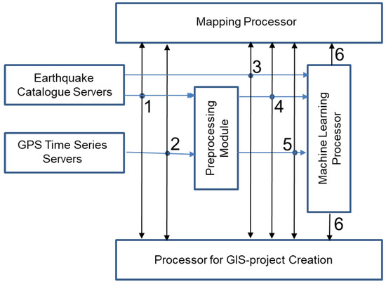
Figure 1.
Scheme of the process of data analysis in GIS Prognosis: 1. Catalog of earthquakes. 2. GPS time series. 3. Catalog of target earthquakes. 4. Seismological spatiotemporal grid fields. 5. Geodynamic spatiotemporal grid fields. 6. Spatiotemporal grid field of alarm.
3.2. GIS Prognosis Functions
GIS Prognosis operates using the Coordinated Universal Time (UTC) standard, converts earthquake catalogs to raster fields, calculates new raster fields, and saves these new rasters as files and images for presentation on the site. This system performs the following set of operations.
- Automatic loading of source data from remote servers. The input data consist of earthquake catalogs and process monitoring time series that represent the preparation of a strong earthquake source. Data from the following websites are used:
- –
- Website of the Kamchatka Branch of the Geophysical Survey of the RAS http://sdis.emsd.ru/info/earthquakes/catalogue.php (accessed on 5 March 2023) [26];
- –
- –
- International Seismological Centre (20XX), On-line Bulletin, https://doi.org/10.31905/D808B830 (accessed on 5 March 2023) [29];
- –
- –
- Nevada Geodetic Laboratory website http://geodesy.unr.edu/about.php (accessed on 5 March 2023) [32].
Earthquake catalog data are updated daily, and GPS data are downloaded with a step. - Preprocessing of input data. Earthquake catalogs are limited by the depth of hypocenters and by the minimum representative magnitude of earthquakes. Time series of receiving GPS monitoring stations are cleaned of noise and processed taking into account data gaps.
- Analysis. Earthquake catalogs and time series are used to calculate grid spatiotemporal fields of forecast features in a universal coordinate grid and with the same time step.
- Training and forecast. Training is performed on all data available at the time of the forecast. As a result of training, the alarm zone is calculated, in which the appearance of epicenters of target events in the interval T is expected.
GIS Prognosis uses the following intuitive data analysis methods:
- Joint visual analysis of maps of time slices of fields with the epicenters of target earthquakes occurring in the interval T of the forecast, and with the epicenters of earthquakes with magnitudes above a given threshold that occurred in the interval T before this forecast;
- Interactive analysis of graphs of time series of values of spatiotemporal fields;
- Tabular and graphical presentation of statistical estimates of forecast quality;
- Preparation of a GIS project for analysis in GIS GeoTime.
3.3. GIS GeoTime Functions
Cartography
- Animated representation of 2D slices of 3D and 4D grid and vector fields;
- Combined animation representation of grid and point spatiotemporal fields;
- Interactive cartographic measurement of grid field values and attributes of vector objects;
- Interactive graphical representation of slices and time series of grid spatiotemporal fields;
- Representation of statistics of interactively selectable polygons of grid fields;
- Management of the palette and dimensions of the cartographic presentation of data.
Preprocessing
- Point Data
- –
- Earthquake catalogs: estimation of minimum representative magnitude and seismic regime parameters, calculation of earthquake sub-catalogs by sorting by magnitude, depth, time, and coordinates;
- –
- Time series: data gap correction, smoothing, parameter estimation.
- Grid Fields
- –
- Calculation of spatial and spatiotemporal grid fields from point marked fields: fields obtained using spatial interpolation, density fields of earthquake epicenters, fields of the slope of the earthquake recurrence graph (b-value) [25], fields of the RTL parameter [33];
- –
- Calculation of spatial and spatiotemporal grid fields from the fields of lines and polygons;
- –
- Grid field filtering: averaging, median smoothing, calculation of derivatives, modulus and azimuth of the spatial gradient, anisotropic smoothing via the AWS method (see Section 4.2.2);
- –
- Evaluation of changes in field values in time and space;
- –
- Estimation of invariants of 2D vector fields: divergence, rotor, shift;
- –
- Estimation of fields of quantiles of values of spatiotemporal fields;
- –
- Grid calculations: calculations on arbitrary algebraic and logical formulas;
- –
- Estimation of the field of field correlation coefficients in a sliding space–time window;
- –
- Estimation of the spatial field of similarity between the time series of the spatiotemporal field and the time series of the same field at an arbitrary point.
Machine learning
- Training and modeling of earthquake prediction using the method of minimum area of alarm.
- –
- Prediction of anomalous objects in spatiotemporal fields;
- –
- Detection of alarm time intervals in spatiotemporal fields;
- –
- Detection of alarm zones at alarm intervals.
- Training in the detection of anomalous geological objects.
The user can perform a series of studies on earthquake prediction with the help of GIS GeoTime tools:
- Study of the effectiveness of earthquake precursors.
- Study of the possibility of increasing the sample size of events for training:
- a
- By adding earthquakes with smaller magnitudes than the target events [23];
- b
- By combining several regions of the same type in terms of seismotectonics and geodynamics.
- Study of the possibility of predicting earthquake magnitudes [24].
- Investigation of earthquake time prediction in a given region.
- Study of spatiotemporal patterns of earthquake precursors.
- Study of the possibility of using universal spatiotemporal attribute fields for earthquake prediction in regions of the same type in terms of seismotectonics and geodynamics.
- Experimental study of physical models of earthquake preparation.
4. Case Studies
4.1. GIS Prognosis
Figure 2 shows the start page of the platform. It allows users to select the analysis region and download GIS GeoTime to their computer. The platform is designed to systematically predict earthquakes in several regions, including California, the Eastern Mediterranean, Japan, and Kamchatka. The earthquake forecasts are based on earthquake catalogs and daily series of surface displacements of the Earth’s surface obtained from GPS observations.
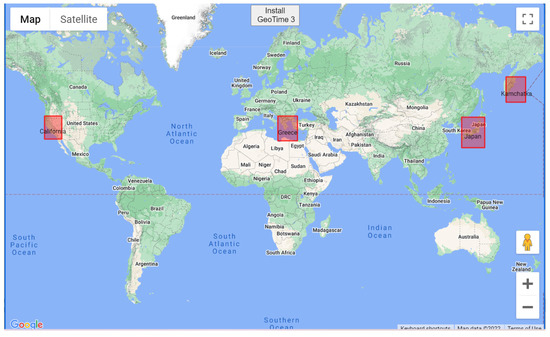
Figure 2.
Starting page of the platform displaying the available regions for selection, including California, the Eastern Mediterranean, Japan, and Kamchatka. The option to download GIS GeoTime is also available by “Install GeoTime 3” button.
Take the California region as an example. Earthquake prediction in the region is based on the earthquake catalog of NEIC and the time series of the daily horizontal surface displacement of the Earth’s surface according to GPS data from the Nevada Geodetic Laboratory site. A comprehensive description of the GPS data utilized is accessible at http://geodesy.unr.edu/PlugNPlayPortal.php (accessed on 17 April 2023). The same portal details how the data is obtained, as described by [32]. We used the “Stations with final solutions” in “env format”, which provides the offset in meters from the reference meridian and equator. Although accuracy data are also provided in the portal, they were not utilized in this study. The properties of the seismic process are represented by space–time fields in a grid of days. The forecast is given for earthquakes with magnitudes .
The analysis zone of the region is the intersection of two zones. The first zone consists of the union of circles with a radius of 100 km, with centers at the nodes of the coordinate grid, which include at least 300 epicenters of earthquakes from 1971 to 1993 with magnitudes from 2.4 and hypocenter depths up to 160.0 km. The second zone consists of a union of 50 km circles with coordinates at the centers of ground stations receiving GPS signals. Machine learning started on 7 August 2009. It is performed automatically with a step days for all data known by the time of each forecast.
A detailed explanation of the grid space–time fields chosen for California earthquake prediction will be given in the next section. These fields (see Section 4.2.1) are (1) the field of change in the average rates of divergence of the deformation of the Earth’s surface in time (field ) and (2) the field of change in the average rates of the shear deformation of the Earth’s surface in time (field ).
In Figure 3 and Figure 4, we present an analysis of the earthquake forecast for the epicenter of the 5.8 magnitude earthquake that occurred on 24 June 2020. Figure 3 shows cross sections of the alarm field (alarm zone) at different forecast intervals. The figures demonstrate the attenuation of the alarm field after three earthquakes in 2019 and the appearance of a new alarm field before the 2020 earthquake. In the interval [16 June 2019–16 July 2019), three earthquakes were predicted on 4 July 2019, 6 July 2019, and 6 July 2019 with magnitudes of 6.4, 7.1, and 5.5 and epicenter coordinates (−117.504, 35.705), (−117.599, 35.770), and (−117.750, 35.901) within the alarm zone. The epicenter of the earthquake on 24 June 2020 with a magnitude of 5.8 and coordinates (−117.975, 36.447) fell into the alarm zone during the interval [10 June 2020–10 July 2020).
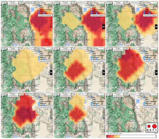
Figure 3.
Sections of the alarm field at forecast intervals: Line 1 [16 June 2019–16 July 2019), [15 August 2019–14 September 2019), [14 October 2019–13 November 2019). Line 2 [11 February 2020–12 March 2020), [11 April 2020–11 May 2020), [10 June 2020–10 July 2020). Line 3 [7 November 2020–7 December 2020), [6 January 2021–5 February 2021), [7 March 2021–6 April 2021). The circles show the epicenters of earthquakes with target magnitudes . In the interval [16 June 2019–16 July 2019), three earthquakes were predicted on 4 July 2019, 6 July 2019, and 6 July 2019, with magnitudes of 6.4, 7.1, and 5.5 and epicenter coordinates (−117.504, 35.705), (−117.599, 35), and (−117.750, 35.901). An earthquake on 24 June 2020, with a magnitude of 5.80 and coordinates (−117.975 36.447) is predicted for the interval [10 June 2020–10 July 2020).
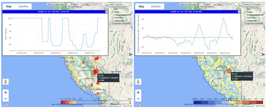
Figure 4.
Analysis of earthquake forecast for a 5.8 magnitude earthquake on 24 June 2020. Left: Alarm zone (10 June 2020–10 July 2020) with earthquake epicenter (red circle center) and plot of alarm field values at the epicenter. Right: Map of the field of increasing divergence values of average strain rate for 360 days (16 June 2019–10 June 2020) compared to the average strain rate for the previous 360 days.
In Section 2, we explained that the alarm field is a function of the predictive feature fields. In our case, and are the feature fields. The alarm field values are an estimate of the probability of a false alarm. The first line of Figure 3 shows a forecast interval in which the alarm zone contains the epicenters of three target earthquakes. The figure demonstrates that in this case, the values of the alarm zone are close to 0, indicating that the values of the attribute fields and are close to anomalous. In the next intervals, the activation of the area shifts to the west. The second line of the figure shows the intervals of the process of activating a new alarm zone, which ends with the occurrence of a target earthquake, the epicenter of which also falls into the alarm zone. The third line of the figure shows the intervals for completing the activation process. The values of the alarm field increase and exceed the threshold value . For values greater than 0.2, the alarm field is not displayed.
Figure 4 illustrates the analysis of the forecast for the epicenter of the earthquake on 24 June 2020 with a magnitude of 5.8. On the left, the figure shows a fragment of the alarm zone map for the forecast interval 10 June 2020–10 July 2020, the epicenter of the analyzed earthquake (the center of the red circle), and the graph of the time series of alarm field values at its epicenter. It can be seen that in the forecast interval, the value of the alarm field is much less than the threshold of the alarm zone, 0.2, and is approximately equal to 0.04. On the right is a map of the time slice of the field of increasing divergence values of the average strain rate in the annual time interval 16 June 2019–10 June 2020 compared to the average strain rate for the previous year. It can be seen that the analyzed earthquake was preceded by a significant anomaly in the increase in the values of the divergence of the average strain rate.
The forecast parameters and statistics are automatically generated using templates and linguistic variables and presented in a file. Part of such a description for the California region is shown in Figure 5.
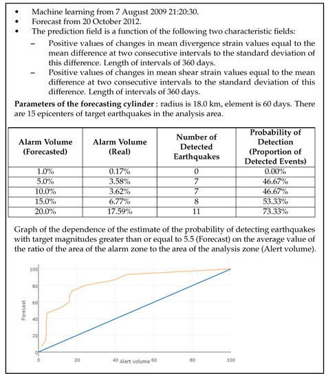
Figure 5.
Fragment of description of the forecast results in GIS Prognosis.
4.2. GIS GeoTime
4.2.1. Performance Analysis of Earthquake Prediction Based on Space Geodesy Fields
Method
Fields are considered effective if they allow obtaining a satisfactory forecast quality. Modeling is performed according to the technique described in [24]. Calculation of the attribute fields of earthquake prediction is performed in two stages. The purpose of the first stage is to extract the useful signal from the time series of the coordinates of the receiving stations. The purpose of the second stage is to identify spatiotemporal fields that are effective for forecasting.
At the first stage, two operations are performed: (1) estimation of the time series of strain rates and (2) calculation of the spatiotemporal grid fields of average daily strain rates with positive values in the west–east and south–north directions. The average daily horizontal displacement rates of the GPS receiving station and are determined by two coordinates separated in time by the interval days: , .
There are discontinuities in the time series of station coordinates. Since the displacement velocity estimates are ahead of the time of the values of the first station coordinates and by days, each gap in the time series of station coordinates increases the number of missing values in the time series of velocity by days. With a large number of discontinuities, the number of missing velocity values can significantly exceed the number of missing coordinate values. To limit the number of gaps in the velocity values, we linearly interpolate coordinate values at gaps less than or equal to . For discontinuities with gaps of more than days, we end the velocity calculation at the last value of the station coordinate before the discontinuity and re-estimate the velocities starting from the first value of the station coordinate after the discontinuity. In [24], the statistics of the values of time series gaps are given, on the basis of which the value of the interval days was chosen.
Spatiotemporal grid fields of daily strain rates and are calculated for the analyzed regions in the grid day. The fields are calculated in two steps. The first step uses an interpolation method known as the inverse distance weighted method. During interpolation, gaps in the values of the time series of daily velocities are taken into account as the absence of a monitoring station. The field values at the grid nodes for each time slice of the west–east velocity component field are calculated via the formula
where is the value of the field of the west–east velocity component at grid node n at time t, K is the maximum number of stations closest to node n, in a circle of radius , is the value of west–east velocity components for the k-th receiving station at time t, is the distance from the k-th station to the grid node n, and p is the degree that determines the dependence of the station weight from its distance to the grid node. The interpolation parameters are km, km, . If , then . The second component of the field is calculated similarly. After interpolation, the values of the velocity fields and are exponentially smoothed with parameters in time days, and in space with a radius of 15 km. Next, the velocity fields are used to calculate the spatiotemporal fields of the strain rate invariants and the fields representing the changes in these invariants in time.
is the divergence field of strain rates. The value of the field at the point with coordinates determines the relative contraction or expansion of the size of a small horizontal area located at this point,
is the field of the strain rate rotor. The value of the field at the point with coordinates determines the direction and intensity of the twisting of the field around the vertical axis located at this point,
is the shear strain rate field. The value of the field at the point with coordinates is determined by the expression
We assume that strong earthquakes can be preceded by anomalous changes not only in the values of the invariants, but also in the values of changes in the deformation regime over time. The values of these fields are equal to the ratios of the average values of the strain invariants over two successive time intervals to the standard deviation of this difference. The field values are calculated in two steps: first, the fields of changes in the deformation invariants in time are calculated with a time step day; then, the fields are converted to the grid days.
Field determines the change in divergence over time. The value of the field at the grid node g is equal to the ratio of the difference between the average divergence values at this grid node on two successive time intervals and to the standard deviation of this difference ,
where is calculated from the values of the field on the interval , and is calculated on the interval .
Field determines the change in the rotor in time. The values of the field are calculated from the values of the field similarly to the values of the field ,
Field determines the change in the shear in time. The values of the field are calculated from the values of the field similarly to the values of the field ,
GPS time series processing operations use a number of parameters: the time interval for estimating average daily displacement rates, the parameters for interpolating time series into spatiotemporal velocity fields, and the sizes of spatial and temporal smoothing windows. The transformation parameters were chosen, as in [22], on the basis of qualitative considerations for the optimal cleaning of signals from noise, methods for restoring missing initial values, and methods for revealing information about the spatial and temporal properties of geodynamic processes.
Modeling
The analysis was performed for the California region. Earthquakes are predicted with an epicenter depth of up to 60 km and a magnitude of . The forecast uses time series of daily horizontal displacements of the Earth’s surface in the west–east and south–north directions in the interval 1 January 2008–5 February 2023. Data are obtained from the Nevada Geodetic Laboratory (NGL) [32]. Fields are considered effective if they allow satisfactory forecast quality to be obtained.
The analysis area (see Figure 6) contains 1204 GPS ground receiving stations. The average minimum distance between receiving stations is 9.38 km, and the standard deviation of these values is 5.74 km. Seismological data are represented by the National Earthquake Information Center (NEIC) [27,28] for the interval of 1 January 1995 to 5 February 2023.
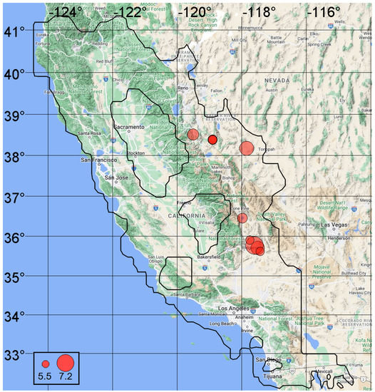
Figure 6.
Analysis zone and epicenters of test earthquakes in the interval 1 January 2008–5 February 2023 with magnitudes and hypocenter depths km.
The parameters of the studied space–time fields , , and , as well as the parameters of the precursor cylinders used in the algorithm of the method of the minimum area of alarm, were selected by us in the training interval before testing for earthquakes with magnitudes in the interval 7 August 2009–2 February 2016.
Analysis of the earthquake precursor efficiency was performed for each of the fields , , , , , and separately. The field is considered effective if, with an alarm volume of no more than , the probability of detecting target events U in the testing interval is statistically significantly different from the probability of detection when predicting by a field consisting of random numbers. The best results of earthquake prediction are obtained from spatiotemporal fields of an increase in time of strain invariants , , and with parameters days. The , , and strain invariant fields, as well as the time decrease fields of , , and strain invariants with the same parameters, showed small estimates of probability for the detection of target events. At the threshold of the alarm, these values are virtually the same as the probability of detecting events via a random field. The parameters of the learning algorithm are equal: the radius of the alarm cylinder is km, and the element of the cylinder is days.
The parameter values that we set as earthquake precursors are not unique to the field under study. The same and more abnormal values can be observed in areas other than the epicenters of the target earthquakes. These zones represent forecast errors, being false alarms. In our case, they are limited by the size of the alarm volume and occupy on average no more than 20% of the analysis area.
Forecasting training was conducted on the interval from 7 August 2009 to the moment of next testing. Testing was carried out between 2 February 2016 and 26 January 2023. Table 1 shows the coordinates of the epicenters of the test earthquakes and the results of the forecast for fields , , and . The forecast card takes alarm values from 0 to 1. Each value of the map corresponds to an alarm volume equal to the share of the alarm area from the area of the analysis zone. The last three columns of Table 1 show the alarms in the test earthquake epicenters. Alarm values of not more than 0.2 are shown in bold type. These earthquakes have been successfully detected with an alarm volume of no more than .

Table 1.
Results of forecasting target earthquakes by spatiotemporal fields of increase in time of strain invariants , and .
Table 1 can be supplemented by the Figure 7 histograms of values of analyzed fields and earthquake harbingers on the test interval. In the figure, the values of the spatiotemporal fields of divergence , rotor , and shear are shown in red. The blue color shows histograms of values of the same fields, which are precursors of 10 test earthquakes. Precursors are the values at the grid nodes of the field that precede the predicted earthquakes at intervals days and refer to cylinders with base centers at the earthquake epicenters and with a base radius km. It can be seen that good histogram separation applies to all fields , , and .
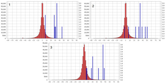
Figure 7.
Histograms of the values of divergence field (1), rotor field (2), and shear field (3), as well as histograms of earthquake precursors, during the testing interval from 2 February 2016 to 26 January 2023 in Japan region. The red bars represent the distribution of field values, while the blue bars show the distribution of earthquake precursor values.
Figure 8 shows the dependencies of the estimated probability of detecting target event U on the volume of alarm V. The experimental data show that the fields of increasing strain rate of divergence , rotor , and shear are almost equally effective for earthquake prediction. However, this conclusion is certainly preliminary. It should be noted that the result was obtained for earthquakes with hypocenter depths up to 12.5 km. The test sample is very small and contains dependent events: a foreshock (line 4, in Table 1) and three aftershocks (lines 2, 3, and 6).
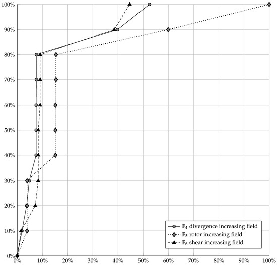
Figure 8.
Plots of dependences in the forecast from the fields of divergence increasing fields, rotor, and shear.
4.2.2. Comparison of Methods to Estimate the Density Fields of Earthquake Epicenters
Method
One of the most important factors in successful earthquake prediction is the method for calculating the space–time fields that carry information about the preparation of target earthquakes. Many precursors of strong earthquakes use the density of earthquake epicenters. In early publications, the spatial density fields of earthquake epicenters were estimated using local kernel smoothing with a sliding cylindrical kernel [33,34]. In later works, the Gaussian kernel function was used instead of a cylindrical window to estimate the spatiotemporal seismic parameter fields [35]. In [36,37], a new method of adaptive weight smoothing of spatial and spatiotemporal fields (AWS) was proposed and studied, and it was subsequently generalized by the authors and called the PS approach (Propagation–Separation). This method is focused on smoothing fields that include areas with locally constant values. The difference from standard methods is that the boundaries between local areas with different constant values are preserved, and the quality of smoothing of field sections with constant values corresponds to standard local kernel methods. AWS generalizes methods of local kernel smoothing, taking into account not only the local features of spatiotemporal data, but also their statistical structure. To take into account the local statistical properties of the data, the method introduces a statistical measure of contrast based on the estimate of the maximum locally weighted likelihood. It was shown in [37] that for a fairly wide class of probabilistic models that belong to the family of exponential-type distributions, the contrast measure is the Kullback–Leibler distance (discrepancy) [38]. In [39,40], the method is generalized to estimate the fields of seismic process parameters from marked point fields, which are, in particular, earthquake catalogs.
Modeling
Let us consider the analysis of the efficiency of earthquake prediction based on the density fields of earthquake epicenters using the data of the Kamchatka region for illustrative purposes. For analysis, we use the earthquake catalog obtained from the website of the Kamchatka Branch of the Geophysical Survey of the Russian Academy of Sciences http://sdis.emsd.ru/info/earthquakes/catalogue.php. The analyzed fields are calculated from the epicenters of earthquakes since 1986, with magnitudes and hypocenter depths km. Earthquake epicenters with magnitudes and hypocenter depths km are predicted. The training starts on 30 March 1998 and ends before the moment of testing. The testing interval is from 29 May 2010 to 20 May 2022. The forecast algorithm has the following parameters: forecasts are generated every 30 days, the radius of the alarm cylinder km, the element of the alarm cylinder days. The analysis area and epicenters of target earthquakes are shown in Figure 9.
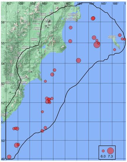
Figure 9.
Analysis area and epicenters of test earthquakes in the interval 29 May 2010–20 May 2022 with magnitudes and depths of epicenters km.
The analysis is carried out on the following three fields:
- is a field of the density of earthquake epicenters, calculated according to the earthquake catalog using Gaussian kernel smoothing. The values of the density field of the epicenters are given bywhere , is the coordinate of the 3D grid node, N is the number of the event, is the magnitude of the n-th earthquake, (km) is the distance from the grid node to the earthquake epicenter, (days) is the time interval from the grid node to the earthquake epicenter, and . The parameters of the formula are as follows: radius km, time interval days, and threshold coefficient .
- is a field of earthquake epicenter density that is calculated using the generalized AWS method [39,40] with the earthquake catalog.
- is a field of earthquake epicenter density that is calculated by smoothing the field using the AWS method [36,37].
Table 2 shows the coordinates of the epicenters of target earthquakes and the results of the forecast for fields , , and . The last three columns of the table show the values of the alarm volume at the epicenters of the target earthquakes. Values of alarm volumes no more than 0.2 are in bold type. These earthquakes were successfully detected with an alarm volume of no more than .

Table 2.
Results of forecasting target earthquakes based on spatiotemporal fields of earthquake epicenter densities , , and .
Table 3 contains estimates of the quality of probability of detecting target events for each of the analyzed fields. Figure 10 shows the dependencies of the estimates of detection probability of target events U on the alarm volume V. It can be seen that the most effective for earthquake prediction in the Kamchatka region are the fields and , for which adaptive weighted smoothing (AWS) was used when estimating the density of earthquake epicenters.

Table 3.
Estimates of prediction of the quality of detecting target earthquakes based on the fields of density of earthquake epicenters , , and . —number of detected target events; U—estimation of detection probability.
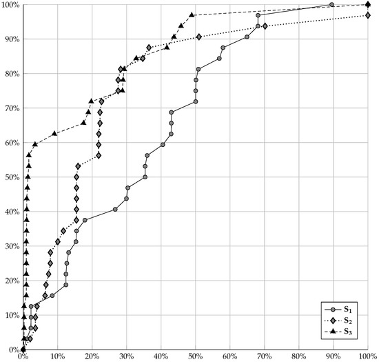
Figure 10.
Plots of dependences in the forecast from the fields (density of the earthquake epicenters with Gaussian Kernel smoothing), (density of the earthquake epicenters with AWS), and (AWS of ).
4.2.3. Modeling Systematic Earthquake Prediction in Japan
Let us consider an example of applying GIS GeoTime to the forecasting of earthquakes in Japan. The area of analysis is limited to the coastline of the Japanese Islands. Usually, the quality of earthquake prediction in this area of analysis, performed only on the basis of seismological data, is found to be lower than for coastal areas. This example illustrates the analysis of the possibility of improving the forecast by adding geodynamic data on the displacements of the Earth’s surface contained in the GPS time series.
We used the GPS time series of daily horizontal displacements of the Earth’s surface in the west–east and south–north directions in the interval 1 January 2009–5 February 2023 and the catalog of earthquakes in Japan. GPS data are from the Nevada Geodetic Laboratory (NGL) [32]. The analysis area contains 1229 GPS receiving stations. The average minimum distance between GPS receiving stations is 12.8 km, and the standard deviation is 5.4. The seismological data of Japan are represented by earthquakes with magnitudes , with hypocenter depths km, taken from the Japan Meteorological Agency earthquake catalogs [30,31] for the interval 21 January 2012–5 February 2023.
The epicenters of earthquakes with magnitudes and hypocenter depths km were chosen as targets. The training began on 21 January 2013 and ended at each step before the moment of testing. The testing interval was from 3 August 2016 to 29 January 2023. The forecast algorithm has the following parameters: the forecast is given every 30 days, the radius of the alarm cylinder km, the element of the alarm cylinder days. The analysis area and epicenters of target earthquakes are shown in Figure 11.
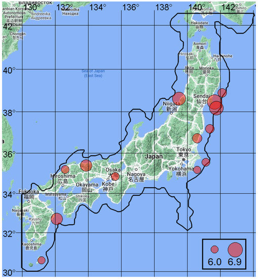
Figure 11.
Japan region: analysis zone and epicenters of test earthquakes in the interval 3 August 2016–29 January 2023 with magnitudes with magnitudes and hypocenter depths km.
Fields and were chosen for the forecast. Field was calculated according to Formula (8) with parameters days, days. The field was calculated using the Gaussian kernel smoothing method. The values of the exponential kernel function are given in (11): (km) is the distance from the grid node to the epicenter, (days) is the time interval from the grid node to the epicenter, , radius km and time interval days, and threshold coefficient . The fields are presented in the grid days.
Table 4 shows the coordinates of the epicenters of test earthquakes and the results of the forecast for fields and . The last two columns show the values of the alarm volume at the epicenters of the test earthquakes, for the forecast performed via only the field and for the forecast performed via both the and fields. Values of alarm volumes no more than 0.2 are in bold type. The earthquakes corresponding to these lines of the table were successfully detected.

Table 4.
Results of forecasting target earthquakes in Japan.
Figure 12 shows the plots of the dependence of the estimate of the probability of detecting target events U on the volume of alarm V. Plot and corresponds to the case wherein the alarm field is built from the fields of increasing divergence of the strain rate () and the density of earthquake epicenters (); plot corresponds to the case wherein the alarm field is plotted only by the density field of earthquake epicenters. It can be seen that with the alarm volume in case and , the estimate of the probability of detecting target earthquakes is , and in case , this estimate is .
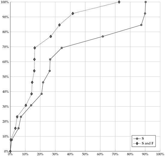
Figure 12.
Plots of dependencies in the forecast for Japan region from fields (density of the earthquake epicenters with Gaussian Kernel smoothing) singly, and both and (divergence increasing fields).
The result of this analysis shows that the addition of GPS data to seismological data can significantly improve earthquake prediction for the area bounded by the coastline of the Japan Islands. From this, it follows that it is necessary to continue the study of earthquake prediction in Japan based on a set of seismological and geodynamic data.
5. Conclusions
In this article, we have presented a new technology for monitoring seismogenic processes and systematically predicting earthquakes. This technology combines geoinformation tools for cartography and data mining and is implemented as a network platform that uses two different types of input data for automatic earthquake prediction. The traditional type of earthquake prediction data are represented by earthquake catalogs that use the coordinates of the epicenter and magnitude of earthquakes for forecasting. The second type is represented by earth remote sensing data that uses the displacement trajectories of ground stations receiving GPS signals for prediction. Our study demonstrates the effectiveness of platform analysis tools that are intuitive and accessible to a wide range of users in solving problems of systematic earthquake prediction. The examples shown in Figure 3 and Figure 4 illustrate that these analysis methods are accessible and informative.
We conducted three examples of data mining on GIS GeoTime and obtained experimental results that show the effectiveness of using space geodesy data for predicting California earthquakes, estimating the density fields of earthquake epicenters using the adaptive weighted smoothing (AWS) method in predicting earthquakes in Kamchatka, and supplementing earthquake catalog data with GPS data on the displacement of the Earth’s surface to improve earthquake prediction for the area bounded by the coastline of the Japanese Islands.
The examples of systematic earthquake prediction in California and the insular part of Japan demonstrate the effectiveness of using space geodesy data for earthquake prediction. The results of the GIS GeoTime application demonstrate that the method of the minimum area of alarm, which was proposed in [21,22,23,24] for machine learning is effective for forecasting, both according to catalog data represented by point fields of earthquake epicenters with an indication of their magnitudes and according to remote sensing data represented by fields trajectories of points on the Earth’s surface.
Author Contributions
Conceptualization, V.G. and A.D.; methodology, V.G.; software, A.D.; validation, V.G. and A.D.; formal analysis, V.G.; investigation, V.G.; resources, A.D.; data curation, A.D.; writing—original draft preparation, V.G.; writing—review and editing, A.D.; visualization, A.D.; supervision, V.G.; project administration, V.G.; funding acquisition, V.G. All authors read and agreed to the published version of the manuscript.
Funding
This research received no funding.
Data Availability Statement
The GPS data were obtained from the Nevada Geodetic Laboratory (NGL), http://geodesy.unr.edu/about.php (accessed on 5 March 2023) at https://doi.org/10.1029/2018EO104623 [32]; the earthquake catalog data for Japan were obtained from the Japan Meteorological Agency (https://www.hinet.bosai.go.jp/) (accessed on 5 March 2023) [30,31]; the earthquake catalog data for California were obtained from the NEIC USGS catalog (https://earthquake.usgs.gov/earthquakes/feed/) (accessed on 5 March 2023) [28]. The earthquake catalog used in this study is produced by the Japan Meteorological Agency, in cooperation with the Ministry of Education, Culture, Sports, Science and Technology. The catalog is based on seismic data provided by the National Research Institute for Earth Science and Disaster Resilience, the Japan Meteorological Agency, Hokkaido University, Hirosaki University, Tohoku University, the University of Tokyo, Nagoya University, Kyoto University, Kochi University, Kyushu University, Kagoshima University, the National Institute of Advanced Industrial Science and Technology, the Geographical Survey Institute, Tokyo Metropolis, Shizuoka Prefecture, Hot Springs Research Institute of Kanagawa Prefecture, Yokohama City, and Japan Agency for Marine-Earth Science and Technology.
Conflicts of Interest
The authors declare no conflict of interest. The funders had no role in the design of the study; in the collection, analyses, or interpretation of data; in the writing of the manuscript, or in the decision to publish the results.
References
- Hyndman, D.; Hyndman, D. Natural Hazards and Disasters; Cengage Learning: Boston, MA, USA, 2016. [Google Scholar]
- Sobolev, G. Principles of Earthquake Prediction; Nauka Publishing House: Moscow, Russia, 1993. [Google Scholar]
- Sobolev, G.; Ponomarev, A. Earthquake Physics and Precursors; Nauka Publishing House: Moscow, Russia, 2003. [Google Scholar]
- Geller, R.J.; Jackson, D.D.; Kagan, Y.Y.; Mulargia, F. Earthquakes cannot be predicted. Science 1997, 275, 1616. [Google Scholar] [CrossRef]
- Koronovskii, N.; Naimark, A. Unpredictability of earthquakes as a fundamental consequence of the nonlinearity of geodynamic systems. Vestn. Mgu. Ser. 4 Geol. 2012, 6, 3–12. [Google Scholar]
- Gufeld, I.; Matveeva, M.; Novoselov, O. Why can not we implement forecast strong crustal earthquakes. Geodin. I Tektonofiz. 2011, 2, 378–415. [Google Scholar] [CrossRef]
- Keilis-Borok, V.; Soloviev, A.A. Nonlinear Dynamics of the Lithosphere and Earthquake Prediction; Springer Science & Business Media: Berlin, Germany, 2013. [Google Scholar]
- Kossobokov, V.; Shebalin, P. Earthquake prediction. In Nonlinear Dynamics of the Lithosphere and Earthquake Prediction; Springer: Berlin/Heidelberg, Germany, 2003; pp. 141–207. [Google Scholar]
- Corbi, F.; Sandri, L.; Bedford, J.; Funiciello, F.; Brizzi, S.; Rosenau, M.; Lallemand, S. Machine learning can predict the timing and size of analog earthquakes. Geophys. Res. Lett. 2019, 46, 1303–1311. [Google Scholar] [CrossRef]
- Shebalin, P.N.; Narteau, C.; Zechar, J.D.; Holschneider, M. Combining earthquake forecasts using differential probability gains. Earth Planets Space 2014, 66, 37. [Google Scholar] [CrossRef]
- Amei, A.; Fu, W.; Ho, C.H. Time series analysis for predicting the occurrences of large scale earthquakes. Int. J. Appl. Sci. Technol. 2012, 2, 1–12. [Google Scholar]
- Marzocchi, W.; Zechar, J.D. Earthquake forecasting and earthquake prediction: Different approaches for obtaining the best model. Seismol. Res. Lett. 2011, 82, 442–448. [Google Scholar] [CrossRef]
- Moustra, M.; Avraamides, M.; Christodoulou, C. Artificial neural networks for earthquake prediction using time series magnitude data or seismic electric signals. Expert Syst. Appl. 2011, 38, 15032–15039. [Google Scholar] [CrossRef]
- Rhoades, D.A. Mixture models for improved earthquake forecasting with short-to-medium time horizons. Bull. Seismol. Soc. Am. 2013, 103, 2203–2215. [Google Scholar] [CrossRef]
- Kail, R.; Burnaev, E.; Zaytsev, A. Recurrent convolutional neural networks help to predict location of earthquakes. IEEE Geosci. Remote Sens. Lett. 2021, 19, 1–5. [Google Scholar] [CrossRef]
- Priambodo, B.; Mahmudy, W.F.; Rahman, M.A. Earthquake Magnitude and Grid-Based Location Prediction using Backpropagation Neural Network. Knowl. Eng. Data Sci. 2020, 3, 28–39. [Google Scholar] [CrossRef]
- Asim, K.M.; Idris, A.; Iqbal, T.; Martínez-Álvarez, F. Earthquake prediction model using support vector regressor and hybrid neural networks. PLoS ONE 2018, 13, e0199004. [Google Scholar] [CrossRef]
- Panakkat, A.; Adeli, H. Neural network models for earthquake magnitude prediction using multiple seismicity indicators. Int. J. Neural Syst. 2007, 17, 13–33. [Google Scholar] [CrossRef] [PubMed]
- Gitis, V.; Derendyaev, A.; Weinstock, A. Web-based GIS technologies for monitoring and analysis of spatio-temporal processes. Int. J. Web Inf. Syst. 2016, 12, 102–124. [Google Scholar] [CrossRef]
- Gitis, V.G.; Derendyaev, A.B. Web-Based GIS platform for automatic prediction of earthquakes. In Computational Science and Its Applications—ICCSA 2018, Proceedings of the 8th International Conference, Melbourne, VIC, Australia, 2–5 July 2018; Springer: Berlin/Heidelberg, Germany, 2018; pp. 268–283. [Google Scholar]
- Gitis, V.; Derendyaev, A. From monitoring of seismic fields to the automatic forecasting of earthquakes. Int. J. Web Inf. Syst. 2019, 15, 535–549. [Google Scholar] [CrossRef]
- Gitis, V.G.; Derendyaev, A.B. Machine Learning Methods for Seismic Hazards Forecast. Geosciences 2019, 9, 308. [Google Scholar] [CrossRef]
- Gitis, V.; Derendyaev, A. The Method of the Minimum Area of Alarm for Earthquake Magnitude Prediction. Front. Earth Sci. 2020, 8, 482. [Google Scholar] [CrossRef]
- Gitis, V.; Derendyaev, A.; Petrov, K. Analyzing the Performance of GPS Data for Earthquake Prediction. Remote Sens. 2021, 13, 1842. [Google Scholar] [CrossRef]
- Gitis, V.; Derendyaev, A.; Petrov, K. On the Applied Efficiency of Systematic Earthquake Prediction. In Proceedings of the Computational Science and Its Applications–ICCSA 2022 Workshops, Malaga, Spain, 4–7 July 2022; Springer: Berlin/Heidelberg, Germany, 2022; pp. 607–624. [Google Scholar]
- Chebrova, A.Y.; Chemarev, A.; Matveenko, E.; Chebrov, D. Seismological data information system in Kamchatka branch of GS RAS: Organization principles, main elements and key functions. Geophys. Res. 2020, 21, 66–91. [Google Scholar]
- Barnhart, W.D.; Hayes, G.P.; Wald, D.J. Global earthquake response with imaging geodesy: Recent examples from the USGS NEIC. Remote Sens. 2019, 11, 1357. [Google Scholar] [CrossRef]
- Masse, R.; Needham, R. NEIC-The national earthquake information center. Earthq. Volcanoes (Usgs) 1989, 21, 4–44. [Google Scholar]
- Bondár, I.; Storchak, D. Improved location procedures at the International Seismological Centre. Geophys. J. Int. 2011, 186, 1220–1244. [Google Scholar] [CrossRef]
- Okada, Y.; Kasahara, K.; Hori, S.; Obara, K.; Sekiguchi, S.; Fujiwara, H.; Yamamoto, A. Recent progress of seismic observation networks in Japan: Hi-net, F-net, K-NET and KiK-net. Earth Planets Space 2004, 56, xv–xxviii. [Google Scholar] [CrossRef]
- Obara, K.; Kasahara, K.; Hori, S.; Okada, Y. A densely distributed high-sensitivity seismograph network in Japan: Hi-net by National Research Institute for Earth Science and DisasterPrevention. Rev. Sci. Instrum. 2005, 76, 021301. [Google Scholar] [CrossRef]
- Blewitt, G.; Hammond, W.C.; Kreemer, C. Harnessing the GPS data explosion for interdisciplinary science. Eos 2018, 99, 485. [Google Scholar] [CrossRef]
- Bune, V.; Gorshkov, G. Seismic Zonation of USSR; Nauka: Moscow, Russia, 1980; p. 307. [Google Scholar]
- Riznichenko, Y.V. On the study of the seismic regime. Izv. Akad. Nauk Sssr Ser. Geofiz 1958, 9, 1057–1074. [Google Scholar]
- Sobolev, G.; Tyupkin, Y.S. Anomalies in the weak seismicity regime prior to Kamchatka strong earthquakes. Vulkanol. Seismol 1996, 4, 64–74. [Google Scholar]
- Polzehl, J.; Spokoiny, V.G. Adaptive weights smoothing with applications to image restoration. J. R. Stat. Soc. Ser. B (Stat. Methodol.) 2000, 62, 335–354. [Google Scholar] [CrossRef]
- Polzehl, J.; Spokoiny, V. Propagation-separation approach for local likelihood estimation. Probab. Theory Relat. Fields 2006, 135, 335–362. [Google Scholar] [CrossRef]
- Kullback, S. Information Theory and Statistics; Courier Corporation: Chelmsford, MA, USA, 1997. [Google Scholar]
- Gitis, V.; Derendyaev, A.; Pirogov, S.; Spokoiny, V.; Yurkov, E. Adaptive estimation of seismic parameter fields from earthquake catalogs. J. Commun. Technol. Electron. 2015, 60, 1459–1465. [Google Scholar] [CrossRef]
- Gitis, V.G.; Derendyaev, A.B.; Pirogov, S.A.; Spokoiny, V.G.; Yurkov, E. Earthquake prediction using the fields estimated by an adaptive algorithm. In Proceedings of the 7th International Conference on Web Intelligence, Mining and Semantics, Amantea, Italy, 19–22 June 2017; pp. 1–8. [Google Scholar]
Disclaimer/Publisher’s Note: The statements, opinions and data contained in all publications are solely those of the individual author(s) and contributor(s) and not of MDPI and/or the editor(s). MDPI and/or the editor(s) disclaim responsibility for any injury to people or property resulting from any ideas, methods, instructions or products referred to in the content. |
© 2023 by the authors. Licensee MDPI, Basel, Switzerland. This article is an open access article distributed under the terms and conditions of the Creative Commons Attribution (CC BY) license (https://creativecommons.org/licenses/by/4.0/).