Mapping Tree Species Using CNN from Bi-Seasonal High-Resolution Drone Optic and LiDAR Data

Abstract

As the importance of forests has increased, continuously monitoring and managing information on forest ecology has become essential. The composition and distribution of tree species in forests are essential indicators of forest ecosystems. Several studies have been conducted to classify tree species using remote sensing data and machine learning algorithms because of the constraints of the traditional approach for classifying tree species in forests. In the machine learning approach, classification accuracy varies based on the characteristics and quantity of the study area data used. Thus, applying various classification models to achieve the most accurate classification results is necessary. In the literature, patch-based deep learning (DL) algorithms that use feature maps have shown superior classification results than point-based techniques. DL techniques substantially affect the performance of input data but gathering highly explanatory data is difficult in the study area. In this study, we analyzed (1) the accuracy of tree classification by convolutional neural networks (CNNs)-based DL models with various structures of CNN feature extraction areas using a high-resolution LiDAR-derived digital surface model (DSM) acquired from a drone platform and (2) the impact of tree classification by creating input data via various geometric augmentation methods. For performance comparison, the drone optic and LiDAR data were separated into two groups according to the application of data augmentation, and the classification performance was compared using three CNN-based models for each group. The results demonstrated that Groups 1 and CNN-1, CNN-2, and CNN-3 were 0.74, 0.79, and 0.82 and 0.79, 0.80, and 0.84, respectively, and the best mode was CNN-3 in Group 2. The results imply that (1) when classifying tree species in the forest using high-resolution bi-seasonal drone optical images and LiDAR data, a model in which the number of filters of various sizes and filters gradually decreased demonstrated a superior classification performance of 0.95 for a single tree and 0.75 for two or more mixed species; (2) classification performance is enhanced during model learning by augmenting training data, especially for two or more mixed tree species.

1. Introduction

Forests, an important part of the global carbon cycle, have played an important role in mitigating climate change caused by global warming [1]. In addition to timber and mining, forests provide temperature regulation, flood protection, and ecosystem management [2,3]. The significant global climate change due to global warming has substantially expanded the global importance of forests. Thus, a 1:5000 scale precision clinical map is created annually in Korea to monitor changes in forest resources and environments [4,5]. Various forest inventories, including tree species, tree diameter, vertical structure, and tree age, are compiled on a specific area to comprehend the current status and distribution of forests nationwide [6]. The composition and distribution of trees in the forest are essential for sustainable forest management and monitoring the conditions of the forest ecosystem [7,8]. It also provides essential information for measuring biomass and carbon absorption in Korea, substantially affecting the establishment of national forest management plans and the determination of fundamental forest statistics [5].

Forest tree species surveys have been conducted through field survey and visual analysis using aerial imagery by experts [9]. Field survey requires considerable resources, such as time, cost, and labor, especially in mountainous areas. Visual analysis results also depend on factors such as the resolution, tree height information, and the experience of the experts conducting the analysis [10]. To overcome these limitations, studies have estimated and classified forest attributes using high-resolution remote sensing data. Drones equipped with sensors are being used to conduct research on forest and vegetation domains in several countries, including the United States, Europe, and China. Using signals, such as optical or microwave radiation, remote sensing systems collect data on objects on Earth’s surface. Because tree species have various spectral reflection and structural characteristics, remote sensing data effectively distinguishes species across a vast area [11,12]. Advancements in drone and sensor technologies have allowed distinguishing between spectral and structural characteristics, increasing the precision of species classification [13].

Deep learning (DL), a machine learning (ML) technology, has been gaining interest because its results are more accurate in tree parameter estimation and classification than other machine learning approaches, such as random forest, gradient boosting, support vector machine, and conventional classification algorithms [14]. The use of convolutional neural networks (CNN), deep learning-based models, in image classification have expanded, owing to their ability to classify complicated patterns within image datasets. The CNN architecture includes a convolution layer and pooling layer for extracting characteristics and compressing the feature maps, respectively. These network architectures use the feature mappings acquired from each convolution and pooling layer to thoroughly train the network [15]. Because the model’s performance changes depending on the network architecture, suggesting an optimal model by combining various convolutional and pooling layers and filters with different architectures is necessary.

As does the network structure, model performance depends on the size and quality of the datasets. Generally, large datasets can increase explanatory power, improve classification accuracy, and minimize overfitting. However, acquiring a significant amount of training data is difficult. The application of augmentation techniques based on the geometric alteration of images overcomes these disadvantages [16,17]. However, according to our review of the literature, quantitative studies on the effects of image augmentation on tree species classification have not been conducted.

Machine learning based tree classification experiments have been conducted on a single tree, and classification performance was enhanced by utilizing discrete spectral data for each tree [18,19]. In the case of labels containing two or more species, such as other broad-leaved evergreen trees and mixed forests, acquiring specific spectral information for each tree is challenging, making reliable classification difficult.

In this study, we conducted a feasibility study on the use of deep learning techniques for tree species mapping by utilizing high-resolution multi-seasonal optical data and LiDAR data collected by drones to investigate the following: (1) the CNN classification performance with various architectures to classify labels including two or more species, as well as a single tree species in a forest, and (2) conducting a quantitative comparative analysis of the image augmentation method for the classification of tree species. For this, we acquired optic and LiDAR data from Jeju Island, South Korea, from the UAV platform on 24 October 2018 and 14 December 2018. To apply UAV optical and LiDAR data to CNN models with various structures, spectral bands such as red, green, and blue and spectral index maps such as the Green Normalized Difference Vegetation Index (GNDVI), normalized difference red edge index (NDRE), and chlorophyll index (CI) were derived from the UAV optical images, and UAV LiDAR data was utilized to generate canopy height maps. To compare the efficacy of data augmentation, we separated the data into two groups; Group 1: before data augmentation and Group 2: after data augmentation using a geometric method. In the end, the performance of forest tree species classification was evaluated and compared to the calculated accuracy of the two groups.

2. Study Area and Data

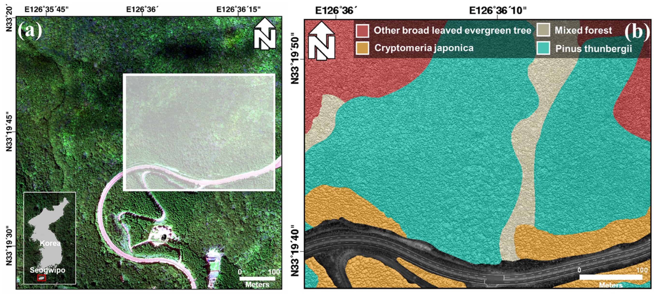
The study area is near Seongpanak on Hallasan Mountain, Seogwipo-si, Jeju Island, South Korea, where cold-resistant and dry-resistant species of broad-leaved evergreen trees have grown. A tree classification map for this study was obtained using a comprehensive vegetation survey in the field. According to the guidelines for classifying tree species in forests in Korea, experts established a stationary quadrat measuring 20 m × 20 m through manual means within the forest. This quadrat was subsequently partitioned into four sections along both its length and width, following which the dominant species present in the region were identified. The dominant species were identified by determining the species with the greatest combined value of relative density, relative frequency, and relative cover. However, if the features were difficult to describe, they were determined by the ecological type of the dominant species and consist of two or more species, such as mixed forests and other broad-leaved evergreen trees. The species shown in Figure 1 were classified as mixed forest, other broad-leaved evergreen trees, Pinus thunbergii, and Cryptomeria japonica. Pinus thunbergii, Machilus thunbergii, and Pinus comprised the mixed forest and Machilus thunbergii and Daphniphyllum were the other broad-leaved evergreen trees. The middle of the study area was a non-forested region, which was a road.

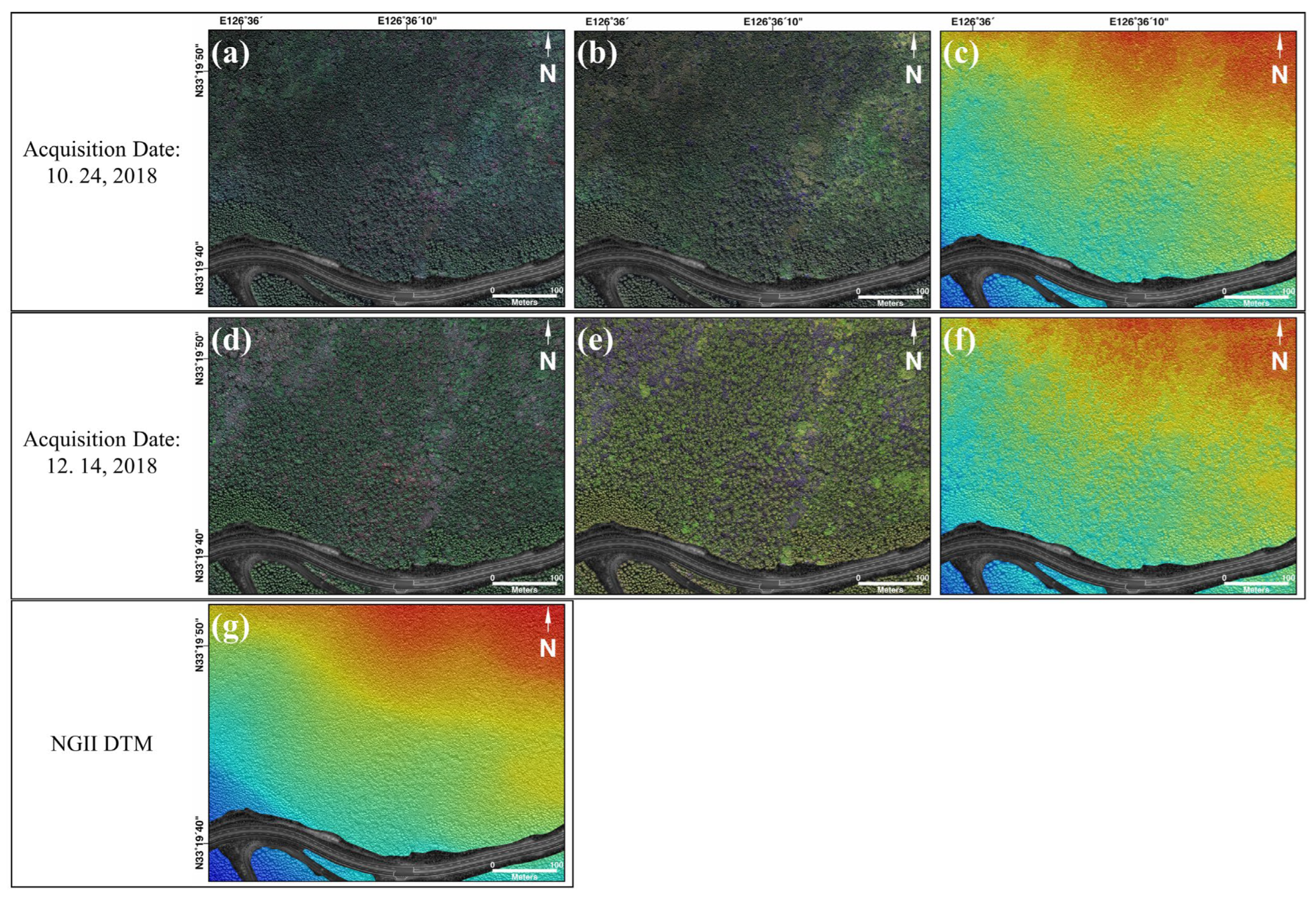
Two-seasonal optic images and LiDAR point clouds acquired by an optic sensor mounted on a UAV platform were used in the study. The first UAV data were acquired on 24 October 2018 (fall) and the second on 14 December 2018 (winter). There is a defoliation period between the two acquisition dates [20]. In addition to deciduous trees, defoliation alters the characteristics of conifers as well. Modifying the acquisition dates is possible. The reason for using October and December data is because in Korea, forestry data is typically collected during the fall and winter months.

The optical images were captured using a FireFLY6 Pro model, which is a fixed-wing drone with vertical takeoff and landing capabilities. The drone has dimensions of 1.5 m in length and 0.95 m in width and weighs 4.1 kg. The UAV optical images mounted on a red edge sensor were captured in the two seasons; five bands were acquired—blue, green, red, red edge, and NIR—on October 24 (fall) and 14 December 2018 (winter) (

Table 1. Specifications of sentinel-2 image.

Bands	Wavelength Center (nm)	Bandwidth (nm)
Blue	475	32
Green	560	27
Red	668	16
Red Edge	717	12
NIR	840	57

). In particular, as chlorophyll absorbs visible and near-infrared wavelengths, resulting in high reflectance values, the application of red edge and NIR offers several advantages for classifying vegetation [21]. Moreover, by combining bi-seasonal images, classification based on intra- and inter-species spectral differences is possible and overcomes the resolution limitations of the sensor spectrum [22]. Their spatial resolution was between 21 and 22 cm, and the orthogonal pictures were resampled to 20 cm using bicubic interpolation.

The LiDAR data was acquired using a rotary wing model known as the XQ-1400VZX drone, as the fixed wing type cannot accommodate the 1 kg LiDAR sensor. The UAV LiDAR data were collected utilizing the Velodyne LiDAR Puck Sensor (VLP-16) with a 3 cm accuracy, and a two-seasonal DSM was produced by manipulating the LiDAR point clouds with TLmaker software. Because the constructed DSM reflects microwaves in the tree area directly below the canopy, height, including artifacts and trees, may be estimated. It was resampled to 20 cm because the spatial resolution of the DSM was approximately 2 cm, and all the images used for DL had the same spatial resolution. For application to DL, all input images had to have the same spatial resolution; therefore, it was resampled to 20 cm from its 2 cm resolution. We also attempted to generate a DTM from LiDAR data but could not obtain an accurate DTM because of the dense forest cover. Therefore, the DTM utilized National Geographic Information Service data. The NGII DTM is a contour-based numerical topographic map that differs from the DSM in terms of vegetation and artifacts. The DTM data were downsampled from 5 to 20 cm. The height of DTM generated using contours can typically be approximated by a smooth surface; hence, resampling to 20 cm has no effect on model performance.

3. Methodology

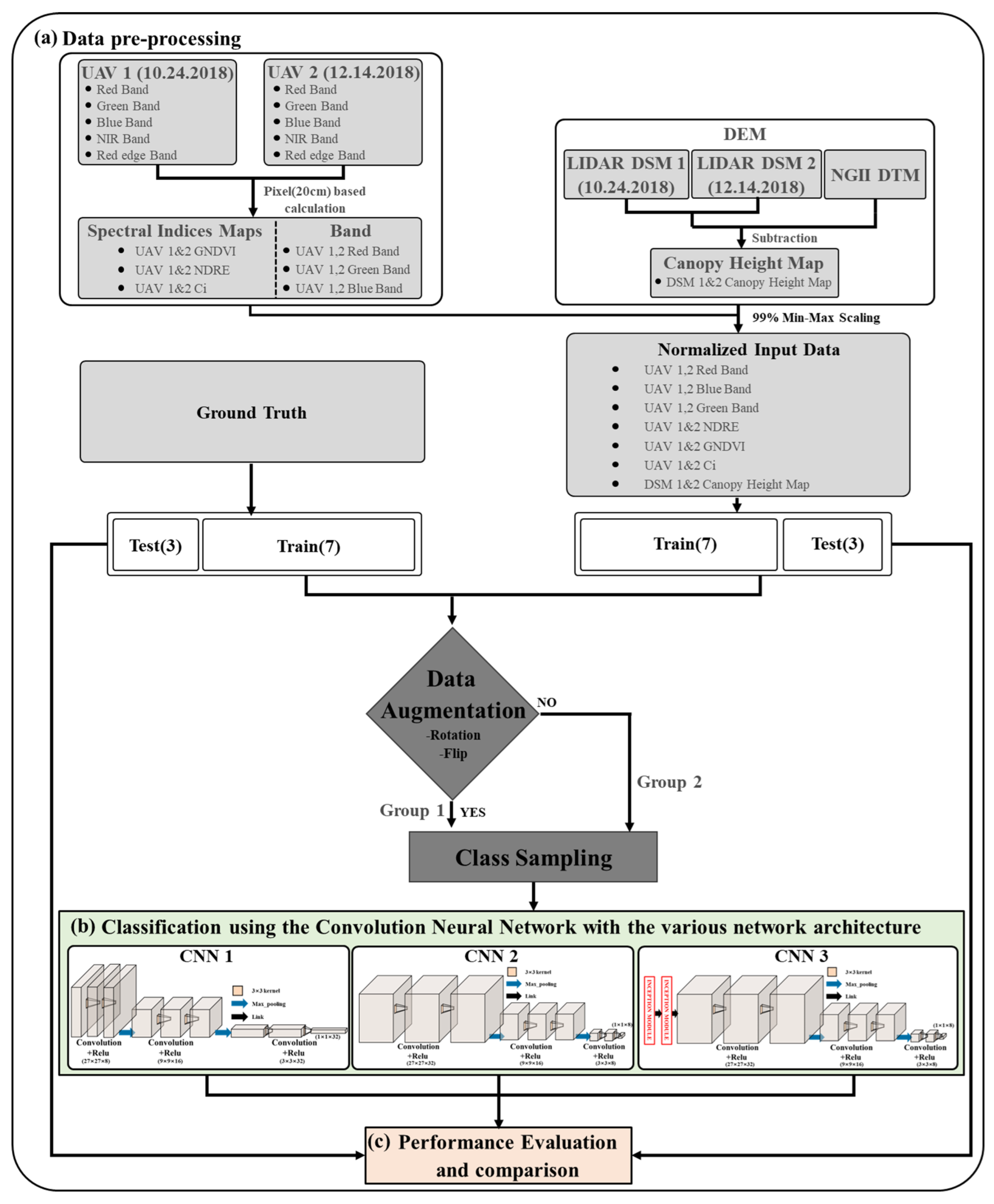
For the feasibility test on the effectiveness of the CNN architecture and data augmentation, the UAV optic and LiDAR data were divided into two groups—before augmentation (Group 1) and after augmentation (Group 2)—and three CNN models were utilized in each group. Subsequently, we used three CNN-based model architectures. The detailed process is illustrated in Figure 2. The primary procedure has three steps: (a) data preprocessing for the trained DL model, (b) classification using the CNN with various network architectures, and (c) performance evaluation and comparison. In the first step, three single standard bands (red, green, and blue) and three spectral index maps (GNDVI, NDRE, and CI) were generated from two time periods of UAV data, and a canopy height map was generated by differentiating the DSM and NGII DTM derived from two time periods of UAV LiDAR data. Subsequently, the maps were normalized using 99% min-max scaling. The normalized maps were randomly and independently split in a 7:3 ratio between training and test datasets. In this instance, the training and test data must be chosen so that they do not overlap in the study region. The training dataset was then separated into Group 1 and Group 2 for a quantitative comparison of image augmentation with or without augmentation. To address the imbalance problem in each class, we ensured that both groups matched the size of each class. Group 1 had 3724 trees per species, a total of 14,896 trees. Group 2 had 8724 trees per species, a total of 34,896 trees. In both groups, 1418 test datasets were obtained. In the second step, the forest tree species were classified using CNN-based models with diverse network architectures for each group. Finally, the classification performance of each group’s three learned models was quantitatively compared and assessed based on the test data using the F1 score and Average Precision (AP) values.

3.1. Generating Input Data

3.1.1. RGB Images and Spectral Index Maps

The red, green, and blue spectral bands are fundamental and affordable data from remote sensing, which have been extensively utilized in vegetation research [23]. Furthermore, various studies have employed RGB images in conjunction with additional data sources, such as spectral index maps and LiDAR data, to enhance the accuracy of classification outcomes [24]. The spectral index map shows the distinction between the absorption and reflectance of each spectral band via the mathematical processing of spectral bands, such as the ratio and difference of spectral characteristics, and is used as an indicator of the relative distribution, activity, leaf area index, chlorophyll content, and photosynthetic absorption and radiation [25]. They involve the reduction of topographic distortion and shadow artifacts in optical image distortion.

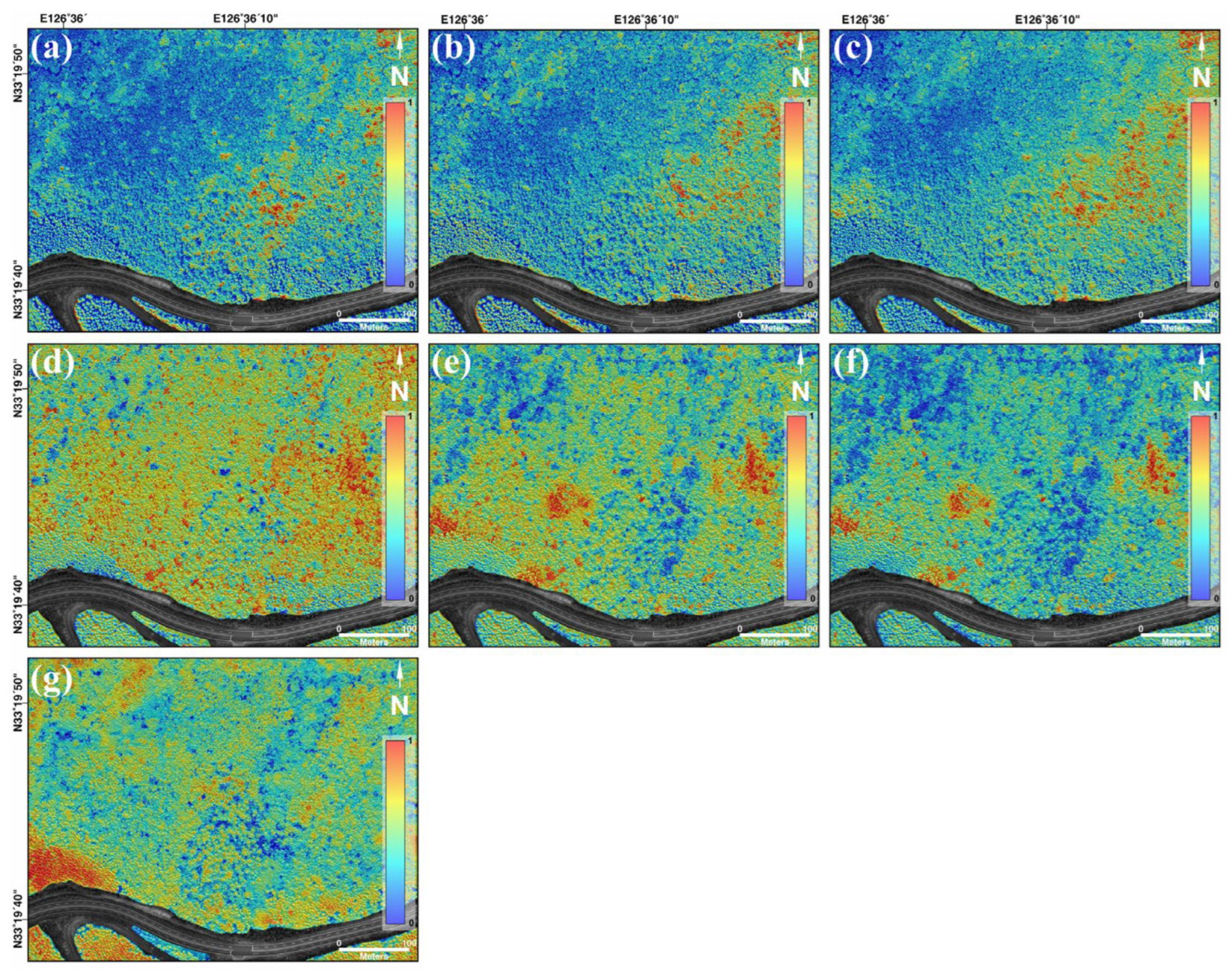
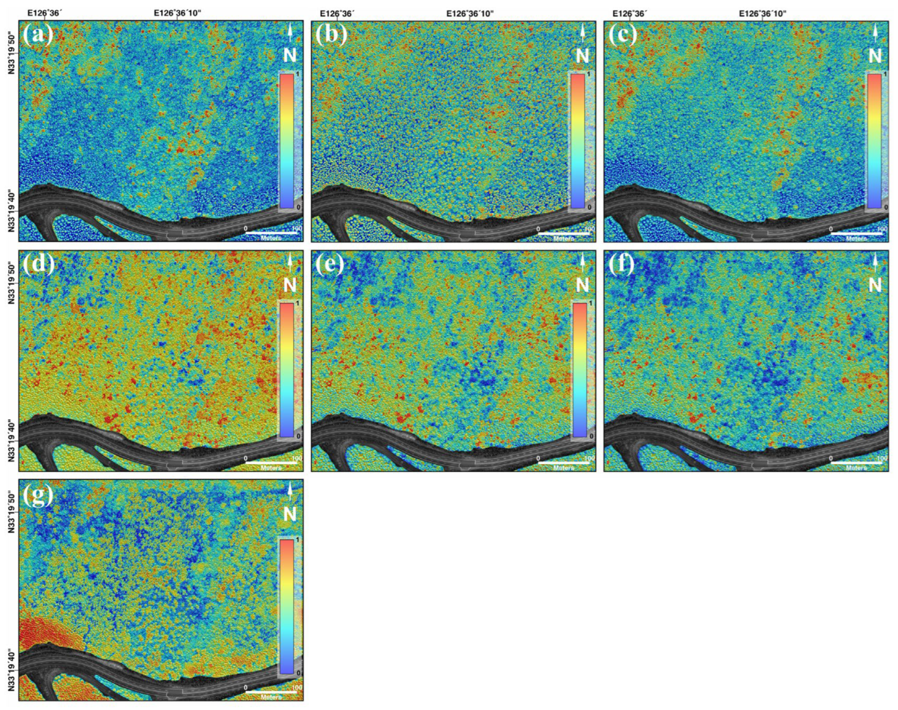
In this study, the overall accuracy of tree classification was improved by integrating individual spectral bands (e.g., red, green, and blue) and vegetation indices (e.g., GNDVI, NDRE, and CI). The expressions for the three vegetation indices used in this study are listed in

Table 2. Information from the spectral index map used in this study.

Name	Abbreviation	Formula
Green Normalized Difference Vegetation Index	GNDVI	(NIR-GREEN)/(NIR + GREEN)
Normalized Difference Red Edge Index	NDRE	(NIR-RED Edge)/(NIR + RED Edge)
Chlorophyll Index (Red edge)	CI	(NIR/RED Edge) − 1

. GNDVI measures canopy variation in the number of green crops in response to variations in crop chlorophyll by using green and NIR band images. In particular, the green channel is sensitive to the visible reflection of chlorophyll and has a linear relationship with biomass and LAI. NDRE is an index that best represents the health and vitality of vegetation. By using the red edge band, the understanding of vegetation vitality can be improved and changes in chlorophyll content can be sensitively indicated, even in situations where the amount of living organisms is saturated. Using the red edge and NIR bands, the CI index was also used to monitor chlorophyll levels and evaluate plant photosynthesis.

3.1.2. Canopy Height Maps

Canopy height maps reflect the structural properties of trees; thereby, they provide valuable information on forest structure, tree species, and other forest properties. As aforementioned, the DSM created by the LiDAR point cloud treatment represents surface height, which includes buildings (artificial objects) and trees on Earth’s surface. In forest areas, microwaves are reflected immediately below the canopy; therefore, it is strongly related to tree height. Alternatively, NGII DTM represents the height of the indicator from which they are extracted. In this study, we determined the height of trees or artifacts by distinguishing DSM and NGII DTM from UAV LiDAR.

3.1.3. Normalization

Normalization describes the technique of standardizing input data by adjusting its scale to account for variations in units and ranges. This prevents deep learning models from overfitting and improves model robustness [26]. In addition, sensor noise due to ambient brightness, noise in the process of compressing the original image, and noise due to transmission errors occur during the acquisition of remote sensing images. Image noise may cause issues such as a reduction in the accuracy of the algorithm. For denoising and normalization, the pixels of the image were sorted by size for each piece of data, and the values corresponding to 0.5% and 99.5% were set as min and max, respectively, and min-max normalization. Normalization values less than 0 were considered 0 and values larger than 1 were considered 1; hence, its range was between 0 and 1. This is used to ensure that each input data is equally important.

3.2. Augmentation

DL models are generated by training parameters, and in the case of CNN, many parameters exist owing to the layering of many layers. Overfitting problems that affect the model’s performance are highly prevalent without sufficient learning data to train the model parameters.

Therefore, training many parameters requires a large quantity of high-quality data, which are difficult to obtain. Several classification studies have improved classification performance through data augmentation techniques to overcome these limitations [27]. So, we incorporated the utilization of data augmentation techniques involving geometric transformations, specifically flipping and rotation, resulting in the acquisition of a substantial quantity of superior training data. Also, we conducted a comparison of the efficacy of high-quality training data. We divided the training data into two groups to determine how the addition of geometric data affected tree species classification. Group 1 did not undergo the augmentation technique and input data were constructed by randomly oversampling each of the 3724 trees to solve the data balance problem by species, including 61% Pinus thunbergii and 8% other broad-leaved evergreen trees. Group 2 randomly sampled data were augmented five times by 90°, 180°, and 270° rotation; horizontal and vertical flip in training data; and was combined with Group 1’s dataset to yield a total of 34,896 training datasets, 8724 in each class.

3.3. Training Classification Model with DL Techniques

DL, developed by simulating human neural networks, is state-of-the-art technology that outperforms other classification algorithms in various image-processing fields, including remote sensing. DL does not require many preprocessing approaches to extract features representing image data because it solves data problems by providing simple intermediate representations that may be combined to form complex concepts [28,29]. Researchers have constructed various neural network designs based on the purpose and type of data, and numerous studies have demonstrated that CNN is optimized for processing image data and outperforms other learning algorithms, such as DNN, MLP, and SVM. CNN solves the problem of spatial features being lost in a fully connected layer when processing image data. Additionally, CNN is constructed through the iterative setting of convolutional and pooling layers, with a final, fully connected layer for classification, in accordance with the user’s intended application. This architecture is commonly referred to as a convolutional neural network.

Specifically, the CNN-based classification model utilized in this study has a different objective than an object detection model such as Yolo, as it is designed to map tree species classification. In addition, as classification of tree species requires a single correct answer value from a single patch, a semantic segmentation model that categorizes correct answer values based on pixels is unsuitable.

CNN Architecture

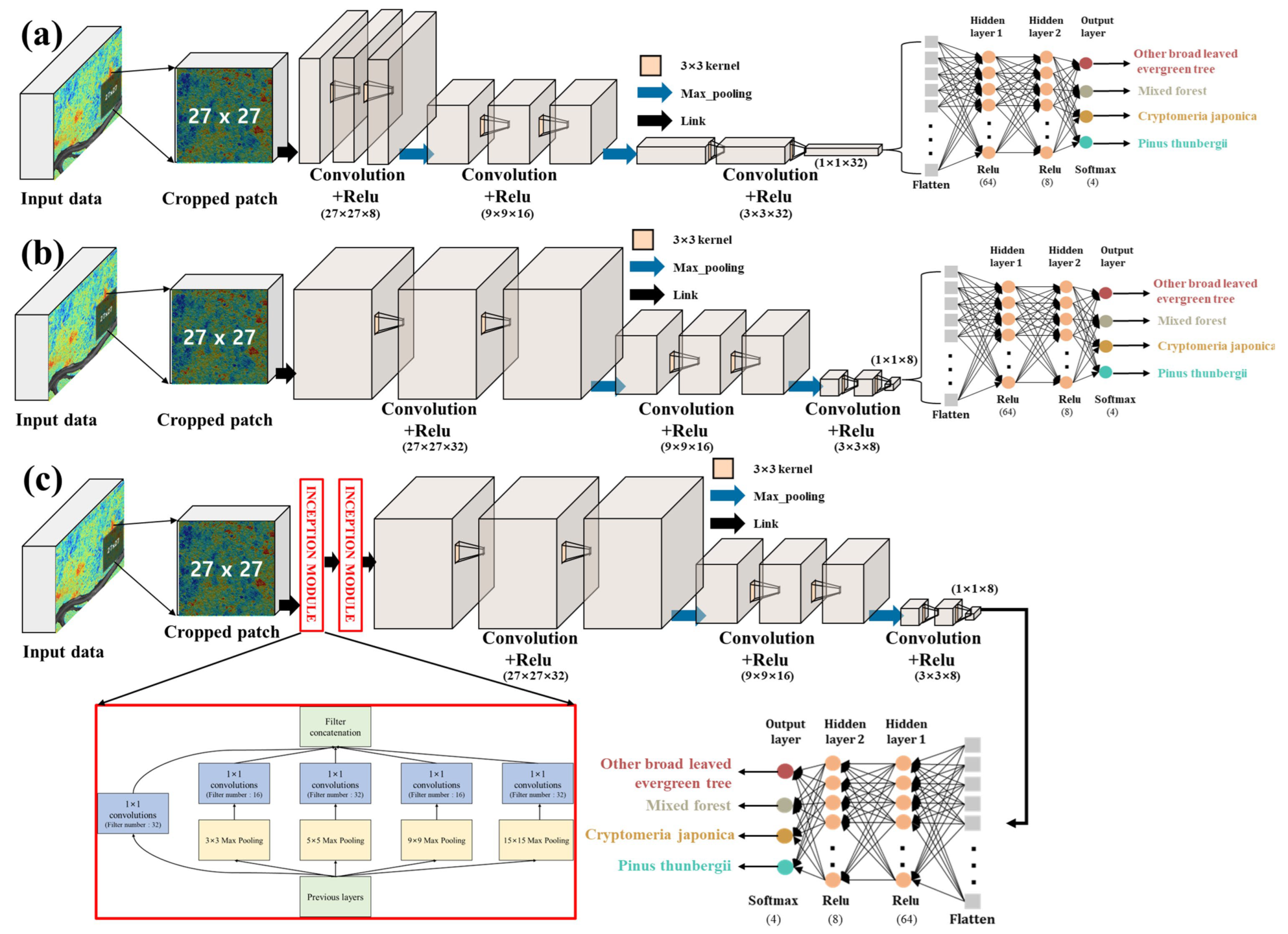
In this study, we compared and examined the performance of tree classification based on the structure of the CNN’s feature extraction area, and we established three models in which the number of feature maps extracted from the number of filters utilized in the convolution computation and generated by the inception module is determined differently for each. Figure 3 shows the prediction process using the CNN classifier used in this study.

In the first model, the number of filters employed in the convolution operation was gradually raised from 8 to 32, generating a small number of feature maps through a small operation at first and employing many feature maps shortly before the fully connected layer.

By contrast, in the second model, the number of filters used in the convolution operation was gradually reduced from 32 to 8, resulting in the creation of many feature maps through multiple operations at the beginning and a smaller number of feature maps before the fully connected layer.

The third model applied the module to the second model. Generally, the greater the number of layers in a neural network, the greater its performance. However, as the number of layers increases, the number of parameters to be learned and the amount of computation required increases exponentially, particularly for image data. Significant research has been conducted on CNN architecture development to improve accuracy and reduce complexity. One of them, the inception module utilized in this work, generated several feature maps by extracting key information from the input data by stacking pooling layers of varying sizes, such as 3 × 3, 5 × 5, 9 × 9, and 15 × 15. Subsequently, a 1 × 1 convolution layer placed the following layer to incur any additional cost, and the number of convolution filters was 32 and 16 iterations, as shown in

Table 3. Inception module hyperparameters.

	Module	Inception Module
Hyper Parameter
Max pooling size		[3 × 3], [5 × 5], [9 × 9], [15 × 15]
Filter size		1 × 1
Convolution filter numbers		[32, 16, 32, 16, 32]

.

Based on the number of convolution and pooling layers and the number of filters applied, the information and size of the resulting feature map vary, which is reflected in the following layer and has a major effect on the model’s performance. For other hyperparameters, the activation function may extract nonlinear data characteristics. The loss function analyzes the model’s performance by indicating the difference between the predictions of the statistical model and the actual results. Depending on the learning rate, the optimizer updates the weights of the DL model to minimize the output value of the loss function.

In this study, three convolution layers and one pooling layer were continually computed using a small 3 × 3 kernel to address nonlinear issues, overfitting concerns, and computational efficiency and to create a higher-dimensional feature map for learning complicated features [30]. ReLU was chosen as the activation function because it may prevent slope loss and reduce overfitting [31]. Adam was applied as an optimizer, and category cross-entropy was exploited using the loss function to categorize several classes. The maximum number of epochs and learning rate were set to 1000 and 0.000001, respectively. The extracted feature map through the convolution and pooling layers was reconstructed by a fully connected layer, and the classification result was generated by a nonlinear activation function (Softmax) in the final output layer. CNN uses two-dimensional input data and the size of the input data influences the classification accuracy of the model. In the case of forest tree species, the size of the patch is 27 × 27, as it measures approximately 5 m² on the image. Except for the number of filters and applications to the inception module, all other hyperparameters in this investigation were applied equally, as shown in

Table 4. Hyperparameters used for CNN-1, CNN-2, and CNN-3 models.

	Module	CNN1	CNN2	CNN3 (Inception Module + CNN2)
Hyper Parameter
Convolution filter number		[8, 8, 8, 16, 16, 16, 32, 32, 32]	[32, 32, 32, 16, 16, 16, 8, 8, 8]
Inception module		-	-	Two times
Number of nodes in fully connected layer		[64, 8, 4]
Convolution filter size		[3, 3, 3, 3, 3, 3, 3, 3, 1]
Convolution filter size		3 × 3
activation		The rectified linear unit (ReLU)
Max pool size		3 × 3
Optimizer		Adaptive Moment Estimation (Adam)
learn rate		0.000001
epochs		1000
Loss function		category cross-entropy
Input data dimension		27 × 27

.

3.4. Performance Evaluation

In this study, quantitative evaluation was performed using the F1 score and the AP value derived from the calculation of precision and recall from the confusion matrix to assess classification performance, according to the group and model [32].

Precision quantifies the proportion of positively labeled samples that are positive, as in (1). Recall estimates the proportion of the positive group that the model correctly estimated as positive, as in (2) [33]. The F1 score is the harmonic mean of precision and recall, taking into consideration both metrics to measure the performance of the classifier model when there are imbalanced class issues, as shown in (3) [34].

$$Precision=\frac{TruePositive}{TruePositive+FalsePositive}$$

(1)

$$\mathrm{Recall}=\frac{True Positive}{True Positive+False Negative}$$

(2)

$$F1 Score=2\ast \frac{Precision\ast Recall}{Precision+Recall}$$

(3)

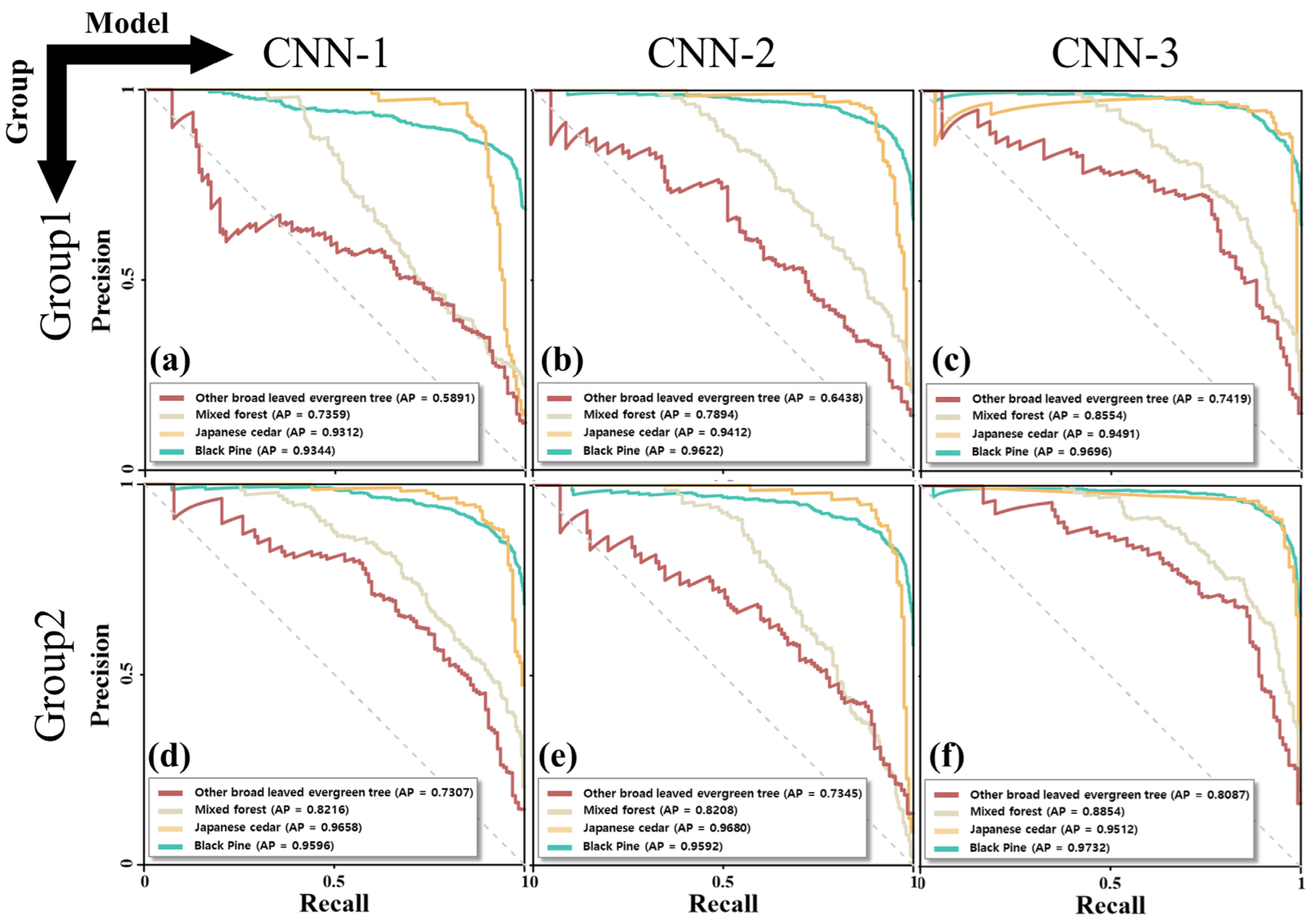
The precision-recall (PR) curve is a graphical representation of the performance of a classification model that considers both precision and recall metrics for different classification thresholds, with the x-axis representing recall and y-axis representing precision. The area under the PR curve, referred to as the AP value, is a useful metric for summarizing the performance of a classifier; a higher AP value indicates that the model is more adept at classification, as shown in (4) [35].

$$AP=\int precision\left(t\right)d\left[Recall\left(t\right)\right]$$

(4)

4. Results and Discussion

4.1. Raw Data

Figure 4 presents the true color composite, false color composite, LiDAR DSM, and NGII DTM images of the study region during autumn and winter. Figure 4a,d are true color images composed of red, green, and blue band images captured on 24 October and 14 December 2018, respectively. Figure 4b,e depicts a false color image derived from red edge, NIR, and blue band images captured on 24 October and 14 December 2018, respectively. The trees are denser in the October image than in the winter image; therefore, Figure 4d,e are superior to a and b for identifying tree boundaries. Moreover, we compared c and f and found that the DSM values have changed as a result of the fallen leaves and the tree’s reduced height. NGII DTM is the height excluding trees and buildings, and the height increases toward the northeast.

4.2. Spectral Index Map and Canopy Height Map

Figure 5 depicts 99% min-max-normalized RGB image data, three index maps (GNDVI, NDRE, and CI), and a canopy height map acquired on 24 October 2018. In the original band images of Figure 5a–c, the Cryptomeria japonica region and Pinus thunbergii in the mixed forest were clearly identified, whereas the overall tree species boundary was divided in Figure 5d–f. In addition, as shown in Figure 5f, the canopy height map provided valuable information for classifying forest species. Particularly notable is the categorization of cedar tree species that comprise artificial forests and other tree species.

Figure 6 shows 99% min-max-normalized RGB image data, three index maps (GNDVI, NDRE, and CI), and a canopy height map collected on 14 December 2018. Figure 6a–c depicts a different perspective from Figure 5a–c. Because the leaves of deciduous trees in other broad-leaved evergreen trees and mixed forests have fallen, the border between tree species has become distinct. Thus, the RGB band was utilized with the index map. The input data consisting of Figure 5 and Figure 6 were used to train a CNN-based model by constructing the learning data for each group.

4.3. Performance Evaluation and Comparison

Figure 7a–c depicts the classification result map for each CNN-based model in Group 1; Figure 7d–f represents the classification result for every CNN-based model in Group 2.

We also present a visual study of several outcomes, which are detailed as follows. First, the CNN-1 classification results are significantly worse than those in CNN-2 and CNN-3. The appropriate size and number of feature maps fluctuate according to the complexity of the training data. However, in the case of species classification from high-resolution images, employing multiple parameter computations to generate many feature maps and to compute the convolution and pooling layers improved the classification results. Second, the classification performance of Group 2 was superior to that of Group 1. This finding was observed owing to the utilization of geometric augmented data to learn from a large quantity of high-quality learning data. Finally, CNN-3 exhibited greater categorization performance than CNN-2, and CNN-3 had greater categorization performance than CNN-2. Bi-seasonal data are utilized for learning, and tree position errors arise when acquiring data from each period [36]. This refers to minimizing the influence of tree position error by acquiring filter information of varying sizes in the inception module.

In Boxes A and B of Figure 7, there are significant discrepancies between the models. Box A is the boundary between Pinus thunbergii and the mixed forest. The CNN-1 model categorized other broad-leaved evergreen trees, Pinus thunbergii, and mixed forests as having ambiguous borders in both groups. CNN-2 and CNN-3 had more distinct borders between the mixed forest and Pinus thunbergii trees than CNN-1. Box B is the boundary between other broad-leaved evergreen trees and Pinus thunbergii, and the dividing line between Groups 2 and 1 is more distinct than that, particularly in CNN-3. In Boxes A and B, misclassification is unavoidable because of the presence of Pinus thunbergii and Machilus thunbergii in the mixed forest and Machilus thunbergii in the other broad-leaved evergreen trees.

Figure 8 depicts the estimated PR curve and AP value for Groups 1 and 2 on the basis of the classification results of the CNN-1, CNN-2, and CNN-3 models. Black, green, orange, and gray lines indicate other broad-leaved evergreen trees, mixed forests, Pinus thunbergii, and Cryptomeria japonica, respectively. The region beneath the PR curve reflects the AP value of the tree species. For the CNN-1, CNN-2, and CNN-3 models within the two groups, the PR curve and AP value of a single tree, Pinus thunbergii and Cryptomeria japonica, demonstrated a high classification performance, whereas other broad-leaved evergreen trees and mixed forests with two or more species demonstrated a relatively low classification performance. When comparing Groups 1 and 2, the classification performance of a single species was similar for all models; however, there was a considerable difference when two or more species were combined.

The AP values of CNN-1, CNN-2, and CNN-3 when two or more species in Group 1 are mixed were approximately at 0.663, 0.717, and 0.79, as shown in Figure 8a–c, and in Group 2, were 0.776, 0.778, and 0.847, respectively, as shown in Figure 8d–f. Group 2 performed categorization approximately 0.113, 0.061, and 0.057 better than Group 1. Additionally, CNN-3 in Group 2 performed better than CNN-1 and CNN-2, with scores of 0.071 and 0.069, respectively. According to the AP value, CNN-3 performed the best classification, whereas CNN-1 performed the worst.

Table 5. Precision, recall, and F1 score for each model and group.

Model	Group	Evaluation Metrics	Other Broad-Leaved Evergreen Tree	Mixed Forest	Cryptomeria Japonica	Pinus Thunbergii	Total
CNN 1	Group 1	Precision	0.54	0.64	0.84	0.88	0.72
		Recall	0.66	0.63	0.90	0.84	0.76
		F1 score	0.59	0.64	0.87	0.86	0.74
	Group 2	Precision	0.58	0.67	0.88	0.91	0.76
		Recall	0.79	0.72	0.94	0.84	0.82
		F1 score	0.67	0.69	0.91	0.87	0.79
CNN 2	Group 1	Precision	0.58	0.75	0.91	0.88	0.78
		Recall	0.60	0.61	0.90	0.93	0.76
		F1 score	0.59	0.68	0.90	0.91	0.77
	Group 2	Precision	0.67	0.63	0.92	0.93	0.79
		Recall	0.69	0.80	0.93	0.85	0.82
		F1 score	0.68	0.71	0.92	0.89	0.80
CNN 3	Group 1	Precision	0.72	0.80	0.92	0.89	0.83
		Recall	0.73	0.69	0.93	0.92	0.82
		F1 score	0.72	0.74	0.92	0.91	0.82
	Group 2	Precision	0.70	0.75	0.89	0.95	0.82
		Recall	0.81	0.84	0.96	0.88	0.87
		F1 score	0.75	0.79	0.92	0.91	0.85

shows the precision, recall, and F1 scores in accordance with the CNN model in each group. The first CNN-3 model achieved the highest precision, recall, and F1 scores in Groups 1 and 2. Consequently, CNN-3 performed the best. Second, throughout all models, Group 2 demonstrated a comparable precision, recall, and F1 score for a single species in Group 1 but a superior recall and F1 score for a mixture of two or more tree species. When two or more tree species were combined, the difference in F1 score was up to 0.09, and the best performance across all evaluation criteria, including precision, recall, and F1 score, was achieved by the CNN-3 model of Group 2. The classification performance measured in terms of F1 score was 0.91 or higher for a single species and 0.75 or higher for a combination of two or more species.

From the results, (1) computing filter information of various sizes, such as the inception module, reduces tree position error effects and has exceptional classification performance for a mixture of two or more species. Therefore, CNN-3 is the best; (2) for mapping tree species classification using CNN-based high-resolution drone images, the structure in which the number of convolutional filters is gradually lowered has a suitable performance; and (3) the construction of input data by geometric data augmentation improves the performance of species classification, particularly a mixture of two or more tree species.

Prior research on classification of forest trees has indicated that the accuracy rate for a singular tree species is approximately 80–90%. However, when dealing with two or more mixed species, such as in a mixed forest and other broad-leaved evergreen trees, the classification accuracy is notably lowered [37]. So, the findings indicates that forest tree categorization maps can be constructed with an accuracy of 0.7 for two or more mixed species and 0.9 for a single tree rousing CNN-3 models trained on both high-resolution optical and LiDAR data after geometric data augmentation.

5. Conclusions

In this study, a methodological strategy for developing models with various CNN structures for high classifiers of forest tree species using multi-time high-resolution optical images and LiDAR data was developed and the impacts of geometric data augmentation were evaluated. In applying bi-seasonal optical images and LiDAR data to CNN approaches, red, green, and blue spectral bands; GNDVI, NDRE, and CI index maps; and canopy height maps were developed and utilized as input data for the three models. In addition, to compare the effects of data augmentation, the input data were separated into two groups: before Group 1 processing and after Group 2 processing. Finally, the learning classification performance was examined and assessed for three CNN models with diverse architectures in the two groups using the F1 score and AP value.

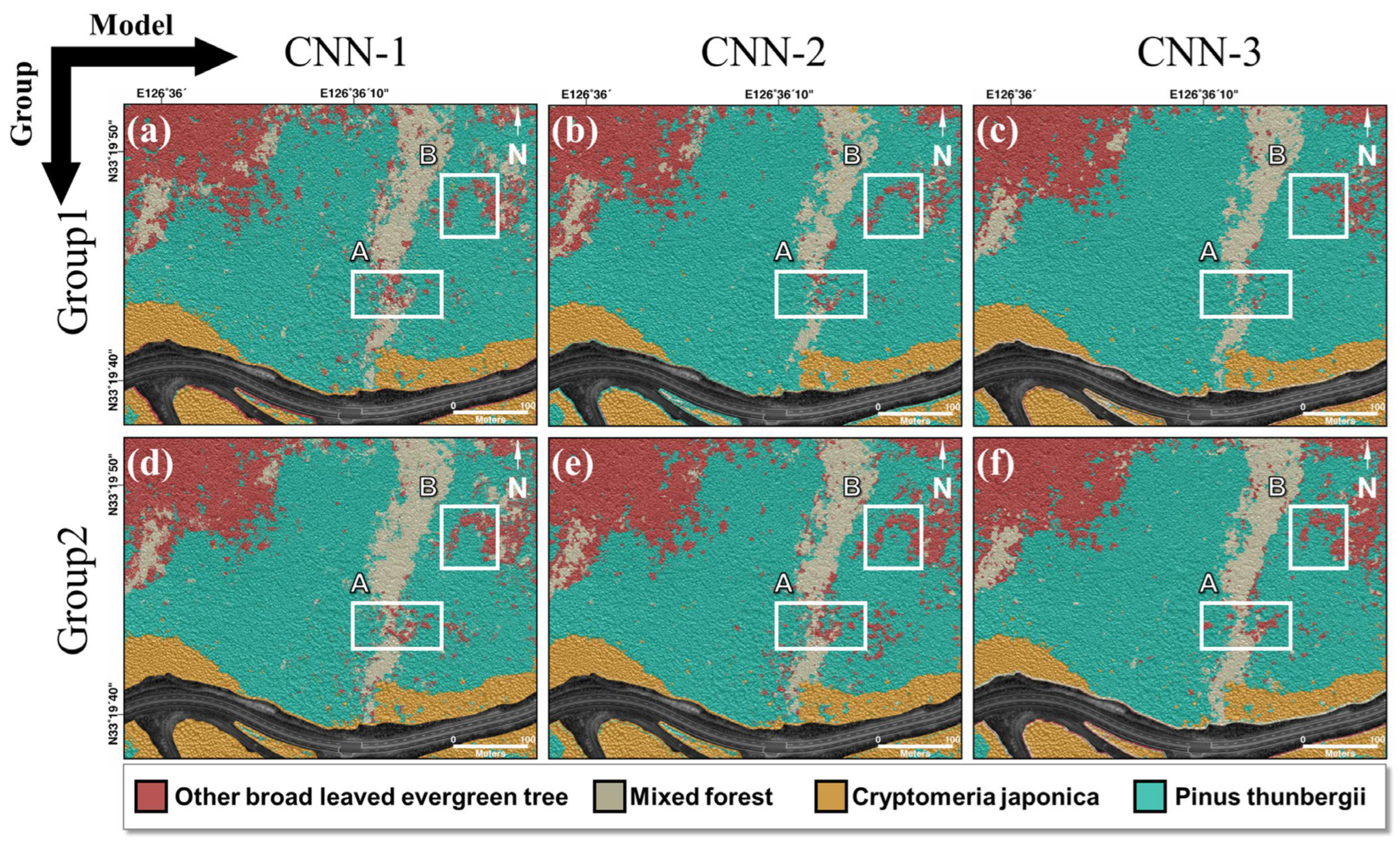
Comparing the AP values of the two groups, CNN-3 performed the best, particularly when two or more species were combined, such as in other broad-leaved evergreen trees and mixed forests. The CNN-1, CNN-2, and CNN-3 values calculated from Groups 1 and 2 were 0.66, 0.72, and 0.79 and 0.78, 0.78, and 0.88, respectively. For Groups 1 and 2, we calculated performance metrics, such as recall, precision, and F1 score, for CNN-1, CNN-2, and CNN-3. In Group 2, the performance indicators were superior to those of Group 1, and Group 2’s CNN-3 model had the best performance with an F1 score of 0.85.

Combining data with geometric data augmentation techniques and CNN-based structures, in which the various filter sizes and the number of filters progressively decrease, suggests that a tree species map with an accuracy of 0.95 or higher for a single species and 0.75 or higher for two or more species is mixed. This shows that, instead of field surveys, a map of forest tree species may be created by applying CNN to high-resolution UAV optics and LiDAR data.