Quantifying the Scale Effect of the Relationship between Land Surface Temperature and Landscape Pattern

Abstract

The spatial scaling of patterns and processes is a hot topic of research in landscape ecology, and different scales may yield completely inconsistent results. Therefore, to understand the impact of the scale effect on urban heat island effect, this study analyzes the correlation between surface temperature and landscape index at different spatial scales over Nanjing. The scale effect is calculated thorough curve fitting of the Pearson’s correlation coefficient between ten landscape indices and land surface temperature at different window sizes, and the optimal one is determined. We have found that landscape indices can be divided into exponential and Gaussian landscape indices whose correlation with land surface temperature at different windows conforms to binomial exponential or multi-Gaussian functions, respectively. The optimal window size is approximately 4000–5100 m for exponential landscape indices, 1000–2000 m for aggregation index (AI) and percentage of like adjacencies (PLADJ), 6330 m for contagion (CONTAG) and 4380 m for total edge contrast index (TECI). Moreover, CONTAG and TECI have a high correlation coefficient plateau where the Pearson correlation coefficient is high and changes by less than 0.03 as the window size changes by more than 3000 m, which makes it possible to decrease the window size in order to save the calculation time without an obvious decrease in the Pearson correlation coefficient. To achieve this, we proposed a suitable window selection function so that the window size becomes 4260 m and 2070 m, respectively. The window sizes obtained in this study are just suitable in Nanjing, but the window sizes in other cities can also be obtained by the method in this study. This study provides a reference for future research on the relationship between landscape pattern and land surface temperature and its driving mechanisms, as well as for the impact of urban land use planning on the heat island effect.

1. Introduction

The urban thermal environment has become a significant concern in light of global warming’s impact on human settlements. Many people in the world are exposed to extreme heat [1]. The urban heat island effect, which occurs as a result of rapid urbanization and expansion, is a growing issue in the Yangtze River Delta region [2]. The negative impact of the urban island on the city is increasing and attracting wide attention. It not only affects the quality of life for residents, but also has a broader impact on urban ecology. The phenomenon of urban heat island makes urban heat islands increasingly a factor affecting urban ecology from general meteorological issues. Urban heat waves, especially when combined with the urban heat island, can result in much more serious heat stress regarding their positive impact on air temperature [3]. The health problems caused by urban heat waves are more serious than those caused by cold [4]. As a result, urban heat island is more intense during a hot day and cause higher health risk, especially for poor people [5]. It makes it much easier for people to obtain diseases such as cardiovascular collapse [6], and even causes death around the world [7,8,9,10,11]. Furthermore, the thermal environment has a profound impact on urban energy and water consumption, ecosystem processes, biological phenology, and the sustainable development of urban economies [12,13,14]. Therefore, addressing the urban heat island effect is an urgent priority.

The urbanization of China has grown rapidly since 1980 and resulted in the increase in urban heat islands [15,16]. Numerous studies have explored the factors and mitigation strategies for the urban heat island effect. Land cover has an obvious relationship with urban heat island [17], and urban green space has been found to effectively lower surface temperature and mitigate the heat island effect [18]. Using geographically weighted regression (GWR) to consider the effect of spatial correlation, Elijah A. Njoku and David E. Tenenbaum [19] found a significant relationship between land use/land cover and land surface temperature. However, maximizing the ecological and environmental benefits of urban green space remains a major focus of current research [20]. Alleviating the urban heat island effect in China by solely relying on increasing the area of urban green space and water bodies is impractical due to limited land availability. To examine the relationship between urban green space layout and the urban heat island effect from a landscape perspective, many scholars have employed landscape ecology methods. Human activities such as urban expansion change the landscape patterns [21]. Therefore, urban planning can adjust the landscape patterns in the city. Landscape patterns have a crucial impact on the urban thermal environment, and the landscape indices we have designed can quantify the aggregation, diversity and connectivity levels of landscape patterns [22,23,24]. Many researchers studied the relationship between landscape indices and land surface temperature with land use data. Sun et al. [25] used the Bivariate Moran’s I method to analyse the spatial correlations of landscape indices and land surface temperature in Chengdu, China. Taking different cities into consideration, Ye et al. [26] studied the correlation between 10 landscape indices and land surface temperature in 5 large cities in China. The results showed that the correlations between landscape indices and land surface temperature is obvious but varied in different cities. Li et al. [27] quantitatively analysed the relationship between configuration landscape indices of greenspace such as mean patch area and land surface temperature intensity by linear regression. They explained the quantitative relationship between landscape indices and the urban heat island effect under high resolution data. In a study using geospatial methods including concentric buffer analysis, correlation analysis, and hierarchical ridge regression model, Ye et al. [26] investigated the impact of landscape patterns on the urban thermal environment in five highly urbanized mega-cities in China. They concluded that arranging urban green space 10–15 km away from the city center maximizes the cooling effect.

However, studies have rarely involved quantifying the scale effect of the correlation between landscape index and urban heat island effect. Wu et al. [28] studied the scale effect on landscape indices and found that the scale effect significantly affected the landscape indices. The values of landscape indices changed under different scales by changing grain size and extent. Wu et al. [29] showed the influence of different scales on the correlations between some of the landscape indices and land surface temperature using the Pearson Correlation Coefficient on the bar graph qualitatively. They demonstrated that the scale effect of correlation of landscape indices and land surface temperature is obvious and vital to the validity of the conclusions of the researchers regarding urban heat island and landscape patterns. Therefore, it is meaningful to use functions to quantify the scale effect of the correlation between land surface temperature and landscape indices in order to design an effective method to look for the optimal window of correlations between landscape indices and land surface temperature to help the researchers when they study the urban heat island. Therefore, this paper uses curve fitting to study the scale effect of the correlation between landscape indices and land surface temperature quantitively. Meanwhile, we propose a method to look for the optimal window.

This paper investigates the scale effect on correlation between 10 different landscape indices and land surface temperature (LST) using remote sensing (RS) and geographic information system (GIS) technology. Taking Nanjing as an example, this study analyses the scale effect of relationship between landscape indices and land surface temperature and find the optimal window sizes. The content includes the following: (1) This paper ses the relationship between landscape indices and land surface temperature by using the Pearson correlation coefficient. (2) This paper quantifies the law of the scale effect of correlation of landscape indices and land surface temperature. (3) This paper provides an optimal window for the correlation between landscape index and land surface temperature in Nanjing. (4) This paper also provides a method of obtaining a suitable window for the correlation between landscape index and land surface temperature, which considers the calculation time and the level of correlation. This finding can aid researchers studying urban thermal environment problems in selecting an appropriate window size.

2. Materials and Methods

2.1. Region of Interest

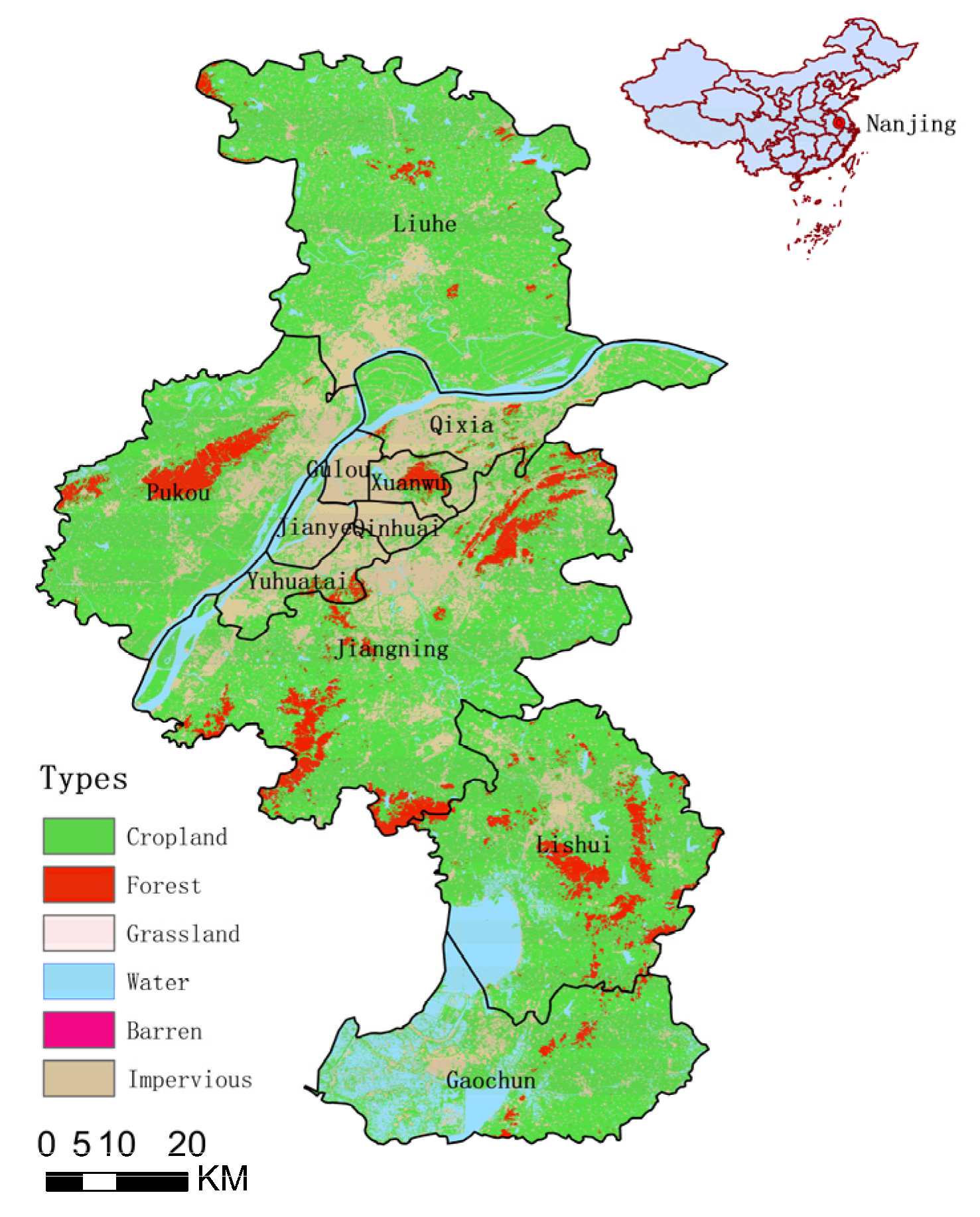
The research data are sourced from Nanjing, a specific region of interest. Nanjing, a city located in the southwestern part of Jiangsu Province, China, is a cultural, political and economic center of the Yangtze River Delta city cluster. It has an administrative area of 6587.02 km², with a built-up area of approximately 868.3 km² by 2020. The city is located in a hilly area, surrounded by mountains on three sides and the Yangtze River to the north. The northern parts of the city are south of the “Laoshan” mountains. Nanjing has a northern subtropical monsoon climate with cold winters, hot summers and high precipitation levels. In 2020, the average temperature was 17.1 °C, and the annual precipitation was 1294.1 mm. The highest temperature in summer can reach 38 °C. The urban area south of the Yangtze River has a high level of modernization, with a dense distribution of high-rise buildings and a large population, bringing huge energy consumption to there. Meanwhile, the mature industrial and commercial activities in the area, along with the increase in cars and consumption levels, have led to urban thermal environment problems. In recent years, with the rapid development of Nanjing Jiangbei District, the urban heat island effect has become increasingly prominent. Figure 1 shows the map of Nanjing.

2.2. Data Source

2.2.1. Land Use Data

The land use cover data utilized in this paper were sourced from the CLCD dataset (https://zenodo.org/record/5816591, accessed on 10 October 2022), which was produced by Huang et al. [30] of Wuhan University. The dataset contains the 2020 Chinese land use cover data with a 30 m spatial resolution. Validation of the dataset was conducted by means of 5463 visual interpretation samples, resulting in an overall accuracy rate of 80%, which is suitable for the research.

Huang et al. [30] used a random forest model to obtain the land use data on Google Earth Engine platform (GEE). The random forest model has been proven to be more accurate and efficient than other machine learning classification methods such as decision tree and support vector machine (SVM) [31]. The theory of random forest model is to build a collection of decision trees to classify the land cover according to the input data. To build decision trees, the random forest model finds the best split according to the traits randomly chosen from input data. The effect of the split is described by Gini coefficient. The smaller the Gini coefficient, the better the effect of the spilt.

$$\begin{array}{c}Gini\left(p\right)={\displaystyle {\displaystyle \sum }_{j=1}^n}{\displaystyle {\displaystyle \sum }_{i=1}^k}{p}_{ij}\left(1-p_{ij}\right) \end{array}$$

(1)

where $n$ is the number of categories generated by the spilt, $j$ is category $j$ generated by the spilt, $k$ is the number of the types of land use cover, $i$ means the land use cover $i$ and $p$ is the frequency of occurrence of land use cover in a category.

The random forest model chooses the split with the smallest Gini coefficient every time to build the decision tree until the number of pixels in leaf node is less than threshold value. Huang et al. [30] built 200 decision trees in their random forest model. When classifying the pixel into land use cover types, the model gives 200 results according to 200 decision trees, respectively. Then, the final result is provided as the result which has the highest frequency occurrence.

To ensure the accuracy of the land use cover results, Huang et al. [31] proposed a method to describe the spatial–temporal consistency probability of a pixel in $3\times 3$ spatial–temporal filter.

$$\begin{array}{c}{P}_{i,t}={\displaystyle \frac{1}{N}}\left[{\displaystyle \sum }_t^{t+2}{\displaystyle \sum }_{x-1}^{x+1}{\displaystyle \sum }_{y-1}^{y+1}I\left(L_{i,t}=L_j\right)\right] \end{array}$$

(2)

where $L_{i,t}$ is the land use cover label of pixel $i$ in the year $t$, $L_j$ is the land use cover label for pixels in the current window, $N$ is the number of pixels in the current window, $I\left(L_{i,t}=L_j\right)$ is 1 if $L_{i,t}$ is equal to $L_j$. Otherwise, $I\left(L_{i,t}=L_j\right)$ is 0. Moreover, $x$ and $y$ are the column and row code of pixel $i$.

When the land use cover changes, the label of pixel should have the spatial–temporal consistency. Huang et al. [30] provided the threshold value of spatial–temporal filter. If $P_{i,t}$ is larger than 0.5, the label of the pixel in year $t$ has a good spatial–temporal consistent. However, if the $P_{i,t}$ is lower than 0.5, the pixel in year $t$ is classified into wrong land use cover type. Then, the label of the pixel $L_{i,t}$ is corrected as $L_{i,t-1}$. Finally, the land use cover data is generated. We download the land use cover data from the website (https://zenodo.org/record/5816591, accessed on 6 October 2022).

2.2.2. Landsat Data

Land surface temperature data with a spatial resolution of 30 m were retrieved by Landsat7 image. Radiometric calibration and atmospheric correction are performed on the image. Then, the image of Landsat7 can be used to retrieve the land surface temperature. Landsat7 is the seventh satellite of the Landsat program in the USA. It has Enhanced Thematic Mapper (ETM+) sensor and was launched in 1999. This paper uses the Level 1 product of Landsat7. We choose the image which was taken on 9 October 2020 at 02:01:30 (Greenwich Mean Time), and the detailed information is shown in

Table 1. The type of landscape indices.

Satellite	Time	Cloud Cover	Resolution	Path/Row
Landsat7	9 October 2020 at 02:01:30 (Greenwich Mean Time)	18%	30 m	120/038

.

2.3. Methods

2.3.1. Land Surface Temperature Retrieving

To ensure the accuracy of the result of land surface temperature retrieving, we use the retrieving algorithm proposed by Cheng et al. [32]. This algorithm can calculate 30 m land surface temperature, which has better accuracy than USGS land surface temperature product [32]. After atmosphere correction, the algorithm can be divided into two steps.

First, calculate the land surface emissivity (LSE) in different land cover types. For non-vegetated surfaces, calculate the land surface emissivity (LSE) in different land cover types. For nonvegetated surfaces, Cheng et al [32] established the empirical equation of land surface emissivity and Landsat SRs.

$${\epsilon }_i=a_0+{\displaystyle \sum }{a}_j\ast {\rho }_j$$

(3)

where ${\epsilon }_i$ is the land surface emissivity, ${\rho }_j$ is the SR of channel $j$. $a_j$ is the parameter of channel $j$, $a_0$ is the constant term.

Then, Cheng et al. [32] proposed a linear regression equation regarding the land surface emissivity of Landsat7 and ASTER.

$${\epsilon }_{L7/b6}=0.278{\epsilon }_{AST13}+0.599{\epsilon }_{AST14}+0.121,R^2=0.975,RMSE=0.003$$

(4)

where ${\epsilon }_i$ is the land surface emissivity of $i$.

Also, the empirical equation of the ASTER emissivity and Landsat SRs can be calculated by statistical regression after spatial-temporal match [32]. Then the empirical equation of land surface emissivity and Landsat SRs is built. We can obtain AST LSE product from https://search.earthdata.nasa.gov/ (assessed on 6 October 2022).

For vegetated surfaces, we use 4SAIL model to build the look-up table of land surface emissivity. In this model, leaf emissivity, soil background emissivity and LAI determine the land surface emissivity [33]. Cheng et al. [32] has provided the range of input parameters of PROSPECT + 4SAIL model, leaf emissivity and soil background emissivity of different land cover types, respectively. They are shown in

Table 2. The emissivity of leaf and soil of different land cover types.

Type	Forest	Shrubland	Savanna	Grassland	Cropland	Other
Leaf emissivity	0.962	0.959	0.968	0.974	0.961	0.965
Soil background emissivity	0.968	0.964	0.964	0.964	0.973	0.968

.

LAI can be calculated by NDVI according to PROSPECT + 4SAIL model, for PROSPECT + 4SAIL model can simulate the surface reflectivity (SR) of red and near-infrared channel of Landsat image [34]. To build the empirical relationship between NDVI and LAI, randomly sample the input parameters and run the model in the range shown in

Table 3. The range of input parameters in PROSPECT + 4SAIL model.

Parameters	Cab	Cbrown	N	Cw	Cm	Car	LAI	Hotspot	Leaf Angle
min	0	0	1.0	6.3 × 10−5	0.0019	0	0	0.01	30
max	100	1	3.0	0.04	0.0165	40	6	0.1	80

. The input parameters include chlorophyll a + b content (C_ab), brown pigment concentration (C_brown), the leaf structure parameter(N), equivalent water thickness (C_w), dry matter content (C_m), carotenoid content (C_ar), LAI, hotspot and leaf angle [32].

Then, we can obtain NDVI from Landsat 7 image and calculate LAI through the empirical relationship between NDVI and LAI. With LAI, leaf emissivity and soil background emissivity, we can calculate the look-up table of land surface emissivity and obtain land surface emissivity by interpolation.

Second, use radiative transfer equation (RTE) algorithm to retrieve the land surface temperature [32].

$$\begin{array}{c}{L}_i=[{\epsilon }_i{B}_i\left(T_s\right)+\left(1-{\epsilon }_i\right)L_i^{\downarrow }]{\tau }_i+L_i^{\uparrow }\end{array}$$

(5)

where $L_i$ is the radiance at sensor of channel $i$, $L_i^{\downarrow }$ is downwelling path radiance of channel $i$, $L_i^{\uparrow }$ is upwelling path radiance of channel $i$, $B_i\left(T_s\right)$ is the blackbody radiance of channel $i$, $T_s$ is land surface temperature which we need to calculate, ${\epsilon }_i$ is land surface emissivity of channel $i$ and ${\tau }_i$ is the atmospheric transmissivity of channel $i$.

We can calculate the blackbody radiance according to the Plank’s law [35].

$$\begin{array}{c}{B}_i\left(T_s\right)={\displaystyle \frac{2h{c}^2}{{\lambda }_i^5\left(e^{{\displaystyle \left(hc/{\lambda }_{i}k{T}_s\right)}}-1\right)}} \end{array}$$

(6)

where $c$ is the speed of light ($2.9979\times {10}^8$ m/s), $h$ is the Planck constant ($6.6261\times {10}^{-34}$ J·S), $k$ is the Boltzmann constant ($1.3806\times {10}^{-23}$ J/K), ${\lambda }_i$ is the effective band wavelength, which is 11.269 $\mathsf{\mu }\mathrm{m}$ for the Band 6 of Landsat 7 [36].

As a result, we can calculate the land surface temperature as follows:

$$\begin{array}{c}{T}_s={\displaystyle \frac{C_1}{{\lambda }_i\ln \left({\displaystyle \frac{C_2}{{\lambda }_i^5\left(B_i\left(T_i\right)-L_i^{\uparrow }-{\tau }_i\left(1-{\epsilon }_i\right)L_i^{\downarrow }\right)/{\tau }_i{\epsilon }_i}}+1\right)}} \end{array}$$

(7)

where $C_i$ is 14387.7 $\mathsf{\mu }\mathrm{m}\cdot \mathrm{K}$, $C_2$ is $1.19104\times {10}^8$ $\mathrm{W}\cdot {\mathsf{\mu }\mathrm{m}}^4\cdot {\mathrm{m}}^{-2}\cdot {\mathrm{sr}}^{-1}$ [26].

The upwelling path radiance, the downwelling path radiance and atmospheric transmissivity can be found on the website https://atmcorr.gsfc.nasa.gov/, accessed on 8 October 2022.

2.3.2. Landscape Index

The relationship between land surface temperature and the degree of aggregation, fragmentation, diversity, shape complexity and connectivity of the landscape has been established in previous studies [37,38,39]. To measure these landscape characteristics, various landscape indices have been developed such as patch cohesion index (COHESION) [26], the aggregation index (AI) [40], Shannon’s diversity index (SHDI) [41], and contagion (CONTAG) [42]. The landscape patterns correlate with land surface temperature [43] and these correlations have been observed in large Chinese cities such as Beijing, Tianjin, Shanghai, Guangzhou and Shenzhen in 1990, 2000 and 2010 [26]. There are also other landscape indices that can describe the spatial distribution of landscape pattern such as connectance (CONNECT), landscape division index (DIVISION), effective mesh size (MESH), modified Simpson’s diversity index (MSIDI), percentage of like adjacencies (PLADJ) and total edge contrast index (TECI) [44]. Thus, this paper selects these landscape indices as the focus of our investigation. We provide a brief description of each landscape index below:

(1) Aggregation Index (AI): The aggregation index reflects the degree of aggregation or dispersion of the same type of landscape patches. The calculation formula is as follows:

$$\begin{array}{c}AI=1+\left({\displaystyle \frac{{{\displaystyle \sum }}_{i=1}^n{{\displaystyle \sum }}_{j=1}^n{P}_{ij}\ln \left(P_{ij}\right)}{2\ln \left(n\right)}}\right) \end{array}$$

(8)

where $n$ represents the number of landscape types, and $P_{ij}$ represents the probability that landscape types $i$ is adjacent to landscape types $j$. The calculation formula is as follows:

$$\begin{array}{c}{P}_{ij}=P_i/P_{j/i} \end{array}$$

(9)

where $P_i$ is the ratio of landscape type $i$’s area to window’s area. $P_{j/i}$ is the probability that a patch is adjacent to another patch whose landscape type is $j$, when the patch’s landscape type is $i$. The calculation formula is as follows:

$$\begin{array}{c}{P}_{j/i}=m_{ij}/m_i\end{array}$$

(10)

where $m_{ij}$ is the number of adjacent edges of patches with landscape type $i$ and landscape type $j$. $m_i$ is the total number of patches whose landscape type is $i$.

(2) Connectance (CONNECT): Connectance measures the degree of connectivity between landscape patches. Strong connectivity between patches facilitates the circulation of material and energy. Since the heat island effect is related to changes in surface energy balance, the connectivity index is expected to be correlated with the heat island effect. The index is calculated using the following formula:

$$\begin{array}{c}CONNECT={\displaystyle \frac{200{{\displaystyle \sum }}_{j=k}^n{c}_{ijk}}{\left(n_i{}^2-n_i\right)}} \end{array}$$

(11)

where $c_{ijk}$ is 1 when the patch of landscape type $j$, and the patch of landscape type $k$ can be connected within the threshold distance. Otherwise, 0. The threshold distance is 100 m in this paper.

(3) Patch Cohesion Index (COHESION): The patch cohesion index represents the degree of aggregation of scenery in space. The calculated formula is follows:

$$\begin{array}{c}COHESION=\left(1-{{\displaystyle \sum }}_{j=1}^n{p}_{ij}/\left({\displaystyle \sum }_{j=1}^n{p}_{ij}\sqrt{a_{ij}}\right)\right)\ast {\left(1-1/\sqrt{A}\right)}^{-1} \end{array}$$

(12)

where $p_{ij}$ is the ratio of the patches of landscape type $ij$. $a_{ij}$ is the number of patches of landscape type $ij$ and $A$ is the total number of patches.

(4) Contagion (CONTAG): Contagion measures the degree of aggregation or diffusion of landscape patches in space. A smaller CONTAG index indicates a more dispersed distribution of different patch types, while a larger index indicates a more clustered distribution of different patch types in space. The index is calculated using the following formula:

$$\begin{array}{c}CONTAG=100\left(1+\left({\displaystyle \frac{{{\displaystyle \sum }}_{i=1}^m{{\displaystyle \sum }}_{k=1}^m{P}_i\left(g_{ik}/{{\displaystyle \sum }}_{k=1}^m{g}_{ik}\right)\ln \left(P_i\right)\left(g_{ik}/{{\displaystyle \sum }}_{k=1}^m{g}_{ik}\right)}{2\ln \left(m\right)}}\right)\right)\end{array}$$

(13)

where $P_i$ is the ratio of the area of the patch whose landscape type is $i$ to the total area. $g_{ik}$ is the number of adjacent patches of landscape type $i$ and landscape type $k$. $m$ is the number of landscape types.

(5) Division Index (DIVISION): Division index shows the dispersion of patches whose landscape type is the same. The calculation formula is as follows:

$$\begin{array}{c}DIVISION=\left(1-{\displaystyle \sum }_{j=1}^m{\left(a_{ij}/A\right)}^2\right)\end{array}$$

(14)

where $a_{ij}$ is the area of patches whose landscape type is $i$. $A$ is the total area of the landscape.

(6) Effective Mesh Size (MESH): Effective mesh size is a metric used to describe the distribution of patch types in space. It is calculated as the ratio of the quadratic sum of patch areas for each landscape type to the total area. The calculation formula for Effective mesh size is as follows:

$$\begin{array}{c}MESH=\left({\displaystyle {\displaystyle \sum }_{j=1}^m}{a}_{ij}^2/A\right)-1/10000 \end{array}$$

(15)

where $a_{ij}$ is the area of the patch, $A$ is the area of the window.

(7) Modified Simpson’s diversity index (MSIDI): Modified Simpson’s diversity index describes the area uniformity of various types of patches in the landscape. The calculation formula is follows:

$$\begin{array}{c}MSIDI=-\mathrm{l}\mathrm{n}\left({\displaystyle {\displaystyle \sum }_{i=1}^n}{p}_i^2\right)\end{array}$$

(16)

where $p_i$ is the probability of the patch whose landscape type is $i$ in the window.

(8) Percentage of Like Adjacencies (PLADJ): Percentage of like adjacencies describes the degree of connection between patches in the landscape. The calculated formula is as follows:

$$\begin{array}{c}PLADJ=\left(g_{ii}/{\displaystyle {\displaystyle \sum }_{k=1}^m}{g}_{ik}\right)\times 100\end{array}$$

(17)

where $m$ is the number of patches. $g_{ii}$ is the number of patches of landscape type $i$ which are connected. $g_{ik}$ is the number of adjacent edges.

(9) Shannon’s Diversity Index (SHDI): Shannon’s diversity index describes the area uniformity of various types of patches in the landscape. The calculation formula is as follows:

$$\begin{array}{c}SHDI=-{\displaystyle {\displaystyle \sum }_{i=1}^m}{p}_i\ln \left(p_i\right) \end{array}$$

(18)

where $p_i$ is the probability of the patches whose landscape type is $i$ in the landscape.

(10) Total edge contrast index (TECI): Total edge contrast index describes the heterogeneity of patch edges in the landscape. The calculated formula is as follows:

$$\begin{array}{c}TECI={\displaystyle \frac{{{\displaystyle \sum }}_{i=1}^m{{\displaystyle \sum }}_{k=i+1}^m\left(e_{ik}{d}_{ik}\right)}{E}}\times 100\end{array}$$

(19)

where $e_{ik}$ is the length of edges of patches whose landscape type is $i$ and patches whose landscape type is $k$. $d_{ik}$ is the weight of the contrast index between the patches of landscape $i$ and landscape $k$. The weight is 1 in this paper.

The scale effect is a common phenomenon in geographic elements. Wu et al. [28] observed a scale effect in the landscape index and emphasized that ignoring this effect can significantly impact the interpretability and practical value of research findings. Estoque et al. [43] discovered a scale effect in the factors influencing the urban thermal environment, where the correlation between impervious surface density and surface temperature was higher at smaller scales. Furthermore, the impact of different scales on land surface temperature varies for each factor. To show the scale effect on the landscape index, this study employs Frastats4.2 software to calculate each landscape index at various window sizes. Windows are selected from small to large including 1000 m, 1200 m, 1500 m, 1800 m, 2000 m, 2200 m, 2500 m, 2800 m, 3000 m, 3200 m, 3500 m, 3800 m, 4000 m, 4200 m, 4800 m, 5000 m, 5200 m, 5500 m, 5800 m, 6000 m, 7000 m, 8000 m, 9000 m, 10,000 m, 11,000 m, 12,000 m, 13,000 m, 14,000 m, 15,000 m, and 16,000 m.

2.3.3. The Calculation of Correlation Coefficient

This paper employs the Pearson correlation coefficient to quantify the relationship between landscape index and surface temperature. A dataset of 15,000 points in Nanjing is selected for this analysis. The calculation method is as follows:

$$\begin{array}{c}{\rho }_{ij}={\displaystyle \frac{Cov\left(LST,X_{ij}\right)}{\sqrt{Var\left(LST\right)}\sqrt{Var\left(X_{ij}\right)}}}\end{array}$$

(20)

where ${\rho }_{ij}$ is the Pearson correlation coefficient between landscape index $i$ and land surface temperature under the window whose size is $j$. $X_{ij}$ is the sample of landscape type $i$ when window size is $j$. $Cov$ means covariance; $Var$ means variance.

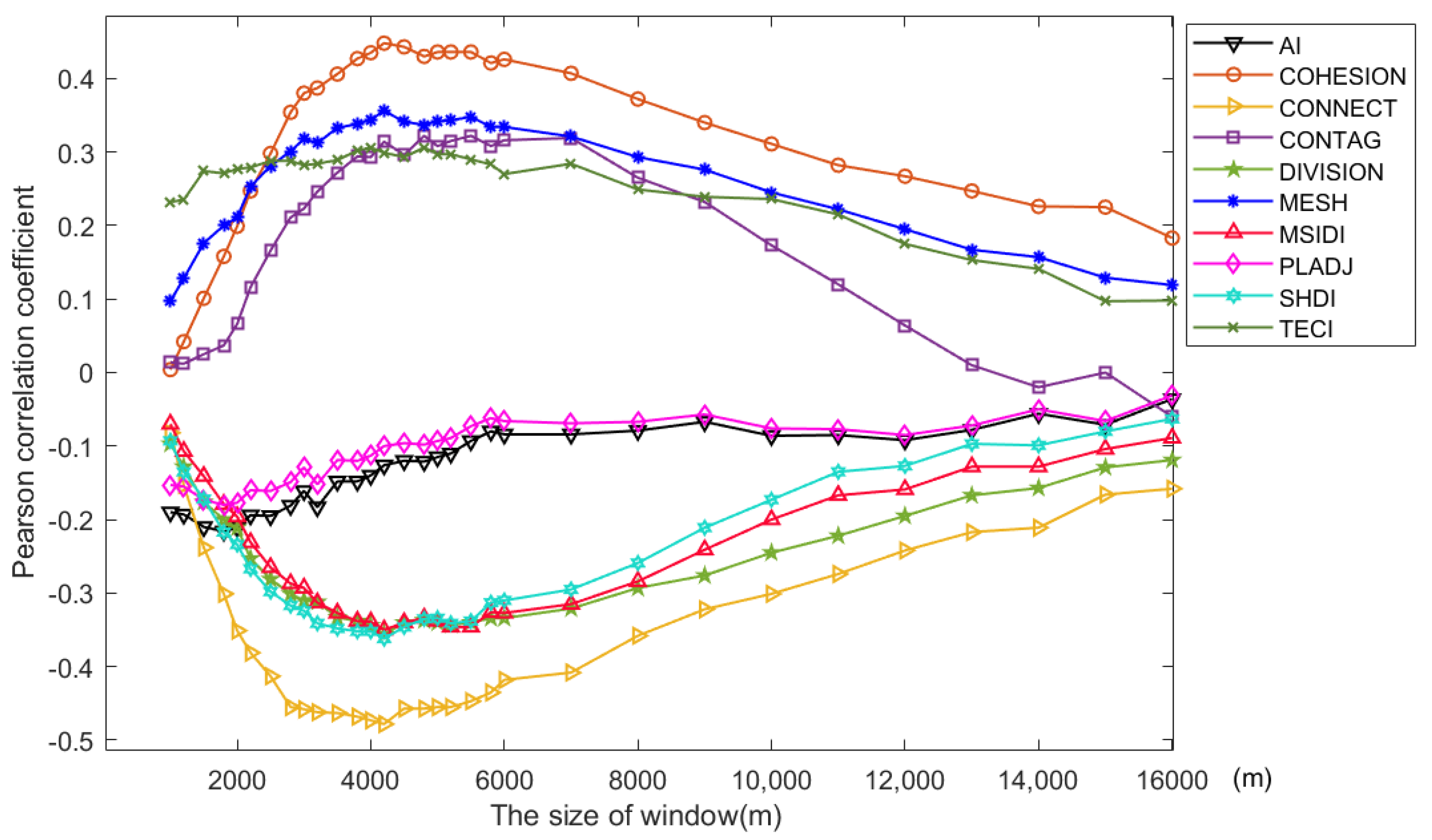
In this study, we utilized SPSS25 software to calculate the Pearson correlation coefficient between land surface temperature and each landscape index for 31 different window sizes. Figure 2 displays the results of these calculations.

2.3.4. Curve Fitting

To explore the correlation between the Pearson correlation coefficient and the window size, this study utilized curve fitting techniques. Various function models were tested, and it was determined that either the binomial exponential function or Gaussian function is suitable for modeling the scale effect of the correlation coefficient. Therefore, these two functions were selected for further fitting. The formula for the binomial exponential function is as follows:

$$\begin{array}{c}y=a{e}^b+c{e}^d\end{array}$$

(21)

where $a$, $b$, $c$ and $d$ are parameters.

The Gaussian function formula is as follows:

$$\begin{array}{c}y={\displaystyle {\displaystyle \sum }_{i=1}^n}{a}_i{e}^{\left(-{\left({\displaystyle \frac{\left(x-b_i\right)}{c_i}}\right)}^2\right)}\end{array}$$

(22)

where $n$ is the number of terms. $a_i$, $b_i$ and $c_i$ are parameters.

To ensure a well-fitted function, limit model complexity and prevent over-fitting, this paper utilizes the adjusted R² and Akaike information criterion (AIC) to determine the number of terms of the Gaussian function. The optimal model is chosen as the one with the smallest AIC value, while ensuring the adjusted R² is not less than 0.95.

2.3.5. Akaike Information Criterion

To determine the optimal number of terms for the Gaussian function fitting, this study uses the Akaike information criterion. This criterion, which is based on the concept of information entropy, helps prevent over-fitting, balance model complexity and improve the model’s application. The optimal number of terms is identified by selecting the AIC value corresponding to the smallest number of terms. The AIC value is calculated using the following method:

$$\begin{array}{c}AIC=2k-n\mathrm{l}\mathrm{n}\left({\displaystyle \frac{S^2}{n}}\right)\end{array}$$

(23)

where $k$ is the number of terms $n$ is the number of samples; $S^2$ is residual sum of squares.

3. Results

3.1. Correlation Analysis between Landscape Index and Surface Temperature

We calculate the Pearson correlation coefficient of landscape indices and land surface temperature and the results are shown in Figure 2.

The results shown in Figure 2 indicate that COHESION, CONTAG, MESH and TECI are positively correlated with surface temperature for the appropriate window size, while AI, CONNECT, DIVISION, MSIDI, PLADJ and SHDI are negatively correlated with land surface temperature for appropriate window sizes. The landscape indices are correlated to the urban thermal environment [40]. The correlation between landscape index and land surface temperature is related to the aggregation and connectivity [40,41], as demonstrated by Equations (8)–(19). COHESION, MESH, MSIDI, DIVISION and SHDI express the aggregation degree of landscape from the perspective of patch area [44], with larger values indicating patches that are closer to a clustered distribution, while larger values of MSIDI and SHDI indicate more dispersed patch distribution. These results showed that the aggregation of building land leads to an increase in local surface temperature, whereas the mosaic distribution of green space between buildings can effectively improve the urban thermal environment [27]. The larger the value of CONNECT, the better the connectivity of similar patches [44], and it has a strongly negative correlation with land surface temperature, indicating that the green corridor formed by the interconnection of green space has an additive effect on improving the urban thermal environment. AI and PLADJ calculate the aggregation of landscape distribution [44] from the perspective of the number of adjacent grids of the same kind, which essentially combines aggregation and connectivity. The positive and negative correlations between AI, PLADJ and surface temperature vary in different regions, suggesting a weak correlation. TECI and CONTAG can be regarded as the aggregation of the landscape pattern calculated by the patch area and the adjacent boundary, with the area being the square of the length of the grid. They have a positive correlation with surface temperature, and the correlation intensity is moderate.

Overall, the correlation between the landscape indices and land surface temperature generally increased and then decreased with increasing window size. COHESION and MESH showed a similar trend, with the maximum correlation occurring at a window size of around 4000–4500 m. In contrast, DIVISION, CONNECT, MSIDI and SHDI showed a negative correlation with surface temperature and peaked at a similar window size. The behavior of AI and PLADJ differed from other landscape indices, with a rise of correlation followed by a plateau, and the maximum correlation appearing at a window size of about 1000–2000 m. CONTAG and TECI showed a high plateau, where the Pearson correlation coefficient changes little. These findings demonstrate a relationship between the correlation coefficient and window size.

3.2. Results of Quantitative Relationship between Correlation Coefficient and Window Size

This paper classifies the landscape indices into correlation coefficient exponential landscape indices and correlation coefficient Gaussian landscape indices according to the model of fitting, which is based on the correlation coefficients between each landscape index and surface temperature under different window sizes.

3.2.1. Correlation Coefficient Exponential Landscape Index

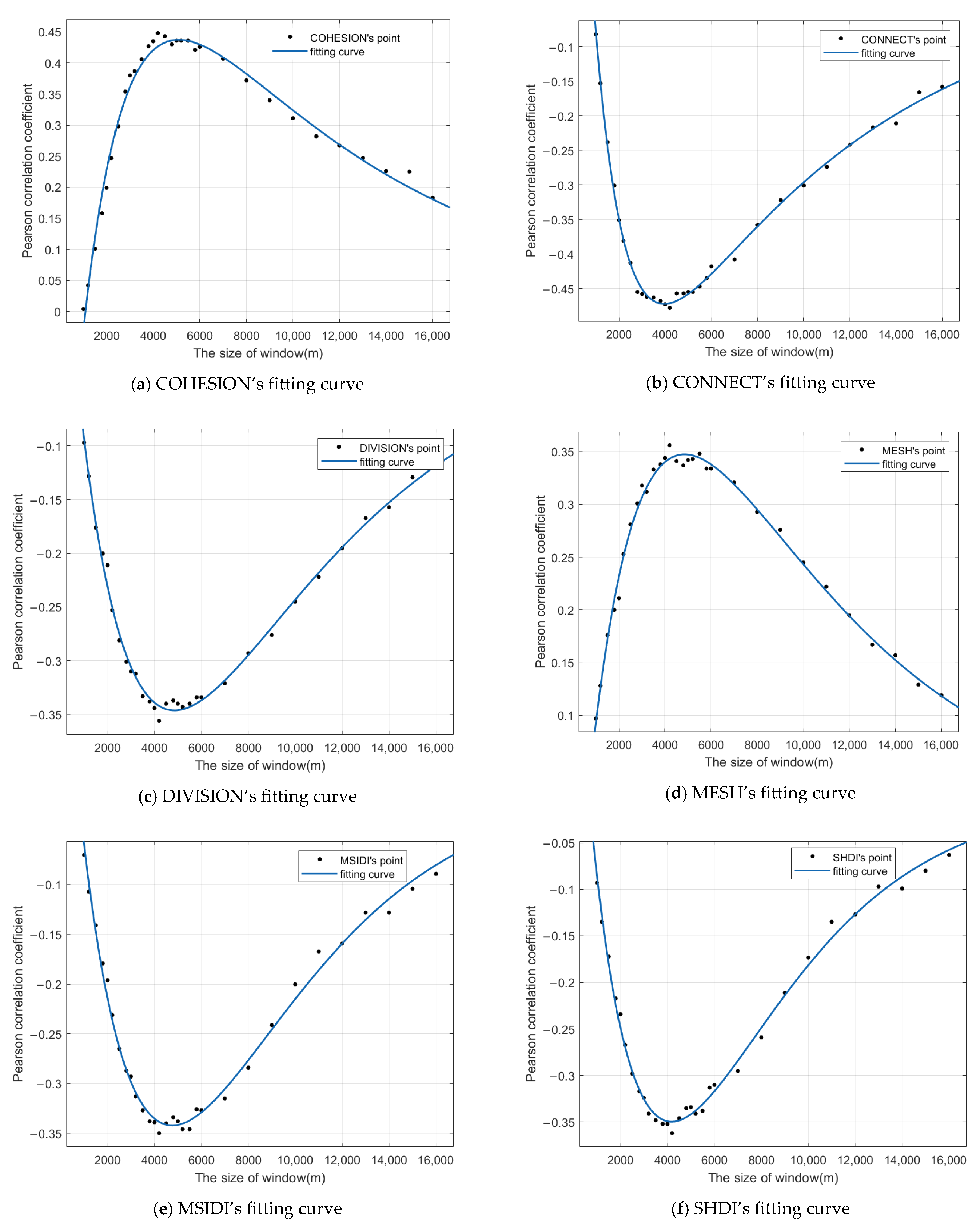
In this paper, the trend of correlation between the correlation coefficient exponential landscape indices and land surface temperature with window sizes is fitted using the binomial exponential function. The resulting curve is shown in Figure 3.

As shown in Figure 3, the function images are U-shaped. COHESION and MESH exhibit a positive correlation with land surface temperature, whereas CONNECT, DIVISION, MSIDI and SHDI display a negative correlation. As the window size increases, the correlation between the exponential landscape index and surface temperature initially increases and then decreases, with the growth rate following a pattern of initial decrease and subsequent increase. We can see the obvious scale effect of relationship between exponential landscape indices and landscape temperature [40].

The curve on the left side of the optimal value has a large tangent slope, indicating a high growth rate of the correlation coefficient. This suggests that when the window size is much smaller than the optimal size, expanding the window appropriately can rapidly improve the correlation between the landscape index and the surface temperature. This rapid growth stage occurs in a wide range of about 1000–4000 m. As the window size approaches the optimal size, the slope of the curve slows down, resulting in a less significant increase in correlation. This stage occurs in a small range of about 4000–5000 m. If the window continues to expand beyond the optimal size, the correlation decreases. The exponential landscape index has a clear global optimal value due to the large range of rapid growth and small range of slow growth. Therefore, the optimal window size for practical applications corresponds to the window size with the maximum correlation coefficient.

To evaluate the fitting goodness of the binomial exponential function, this paper employs adjusted R-squared. The values of adjusted R-squared for the correlation between each landscape index and surface temperature are presented in

Table 4. Fitting goodness of correlation coefficient exponential landscape index.

Landscape Index	COHESION	CONNECT	DIVISION
Adjusted R2	0.9841	0.996	0.993
landscape index	MESH	MSIDI	SHDI
Adjusted R2	0.9925	0.9901	0.9925

.

Table 4 presents the adjusted R-squared values for the correlation between each landscape index and surface temperature, all of which are greater than 0.98, indicating a strong fitting goodness of the binomial exponential function. This model accurately represents the quantitative relationship between the correlation coefficient, calculated by the exponential landscape index, land surface temperature and window size.

The expressions of the Pearson correlation coefficient and the window size are as follows:

$$\begin{array}{c}{\rho }_{COHESION}=0.9251e^{-0.000102x}-1.422e^{-0.0004971x}\end{array}$$

(24)

$$\begin{array}{c}{\rho }_{CONNCET}=-0.8208e^{-0.0001016x}+1.378e^{-0.0007295x}\end{array}$$

(25)

$$\begin{array}{c}{\rho }_{DIVISION}=-1.054e^{-0.0001348x}+1.194e^{-0.0003667x}\end{array}$$

(26)

$$\begin{array}{c}{\rho }_{MESH}=1.059e^{-0.0001353x}-1.202e^{-0.0003675x} \end{array}$$

(27)

$$\begin{array}{c}{\rho }_{MSIDI}=-25.45e^{-0.0002423x}+25.65e^{-0.0002531x}\end{array}$$

(28)

$$\begin{array}{c}{\rho }_{SHDI}=-2.691e^{-0.0002289x}+2.904e^{-0.0003459x}\end{array}$$

(29)

where $x$ is window size and $\rho$ is the Pearson correlation coefficient of exponential landscape index and land surface temperature.

It can be seen from the expressions that each exponential landscape index has a unique optimal window size that corresponds to the maximum correlation coefficient with land surface temperature. Although the optimal window size is similar across different indices, the expression of each index varies significantly, for various landscape indices describe different aspects of landscape pattern and are calculated variously [44]. This indicates that the scale effect of the correlation between exponential landscape indices and land surface temperature is unique and depends on the calculation formulas and the meaning of the indices. Therefore, different exponential landscape indices have different optimal windows, which can be determined by their expressions, providing the most suitable window size for studying the urban heat island effect.

3.2.2. Correlation Coefficient Gaussian Landscape Index

To determine the number of Gaussian function terms for each Gaussian landscape index, the AIC is utilized, which takes into account both the goodness of fit and model complexity. A smaller AIC value indicates a better model.

Table 5. The table of terms number of Gaussian landscape index.

Landscape Index	AI	CONTAG	PLADJ	TECI
The number of terms	2	4	2	3
AIC value	−291.6404	−304.2682	−292.1786	−304.6713

displays the number of terms determined by the AIC and their corresponding AIC values.

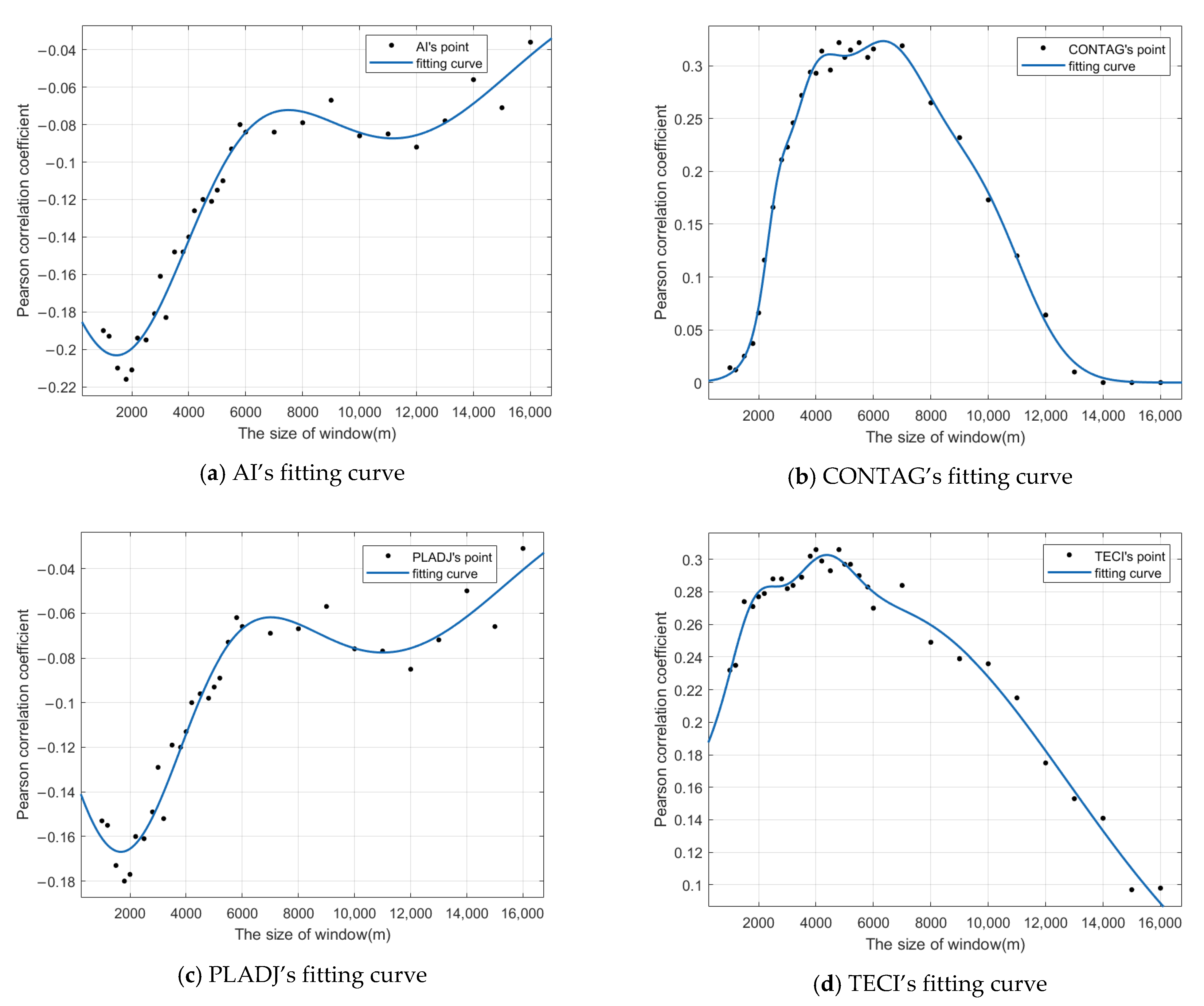
The best Gaussian models for the aggregation index (AI), contagion (CONTAG), percentage of like adjacencies (PLADJ) and total edge contrast index (TECI) were determined to have 2, 4, 2, and 4 terms, respectively. The results of fitting are presented in Figure 4.

The scale effect of correlation between Gaussian landscape indices and land surface temperature is also obvious [40], as shown in Figure 4. The aggregation index (AI) and percentage of like adjacencies (PLADJ) exhibit similar correlation scale effects with land surface temperature. The curves display wavy fluctuations and reach significant optimal values earlier. Conversely, contagion (CONTAG) and total edge contrast index (TECI) exhibit different scale effects. Both curves have a high correlation platform of about 4000 m, with CONTAG exhibiting a high correlation plateau of about 4000–7000 m, and TECI exhibiting one of about 2000–6000 m, where the Pearson correlation coefficient of landscape indices and land surface temperature changes by less than 0.03 as the window size changes by more than 3000 m.

The goodness of curve fitting can be assessed by the adjusted R² value, which is used in this study to evaluate the fitting effect.

Table 6. The table of fitting effect of Gaussian landscape index.

Landscape Index	AI	CONTAG	PLADJ	TECI
Adjusted R2	0.9683	0.9913	0.9518	0.9804

presents the adjusted R² values for the Gaussian landscape index, providing an indication of the degree of fit between the data and the model.

Based on the results presented in Table 6, it can be inferred that the adjusted R² value is greater than 0.95, indicating that the model has a good fitting goodness. Therefore, the Gaussian function has effectively described the quantitative relationship between the correlation coefficient of the Gaussian landscape index, surface temperature and the window size.

The expressions of quantitative relationship between the correlation coefficient and the window size are as follows:

$$\begin{array}{c}{\rho }_{AI}=-0.199e^{-{\left(\frac{x-1356}{3874}\right)}^2}-0.08704e^{-{\left(\frac{x-11250}{5662}\right)}^2}\end{array}$$

(30)

$$\begin{array}{c}{\rho }_{CONTAG}=0.3067e^{-{\left(\frac{x-6256}{2583}\right)}^2}+0.1434e^{-{\left(\frac{x-9797}{2246}\right)}^2}\\ +0.1677e^{-{\left(\frac{x-3685}{1360}\right)}^2}+0.05507e^{-{\left(\frac{x-2624}{549.8}\right)}^2}\end{array}$$

(31)

$$\begin{array}{c}{\rho }_{PLADJ}=-0.1593e^{-{\left(\frac{x-1540}{3346}\right)}^2}-0.0776e^{-{\left(\frac{x-11020}{6177}\right)}^2}\end{array}$$

(32)

$$\begin{array}{c}{\rho }_{TECI}=0.04397e^{-{\left(\frac{x-4096}{1580}\right)}^2}+0.05316e^{-{\left(\frac{x-1817}{1120}\right)}^2}+0.2697e^{-{\left(\frac{x-6175}{9317}\right)}^2} \end{array}$$

(33)

where $x$ is window size and $\rho$ is the correlation coefficient of Gaussian landscape index and land surface temperature.

From the fitting curve, aggregation index (AI) and percentage of like adjacencies (PLADJ) were found to have similar correlations with land surface temperature. Therefore, when constructing a model for land surface temperature, only one index should be used. However, contagion (CONTAG) and total edge contrast index (TECI) showed different scale effects on the correlation with land surface temperature, although they shared the characteristic of a high plateau where the Pearson correlation coefficient is high and changes little as the window size changes.

3.3. Optimal Window Calculation

3.3.1. Optimal Window of Correlation Coefficient Exponential Landscape Index

This paper adopts the window size corresponding to the global optimal value on the fitting curve of the exponential landscape index as the optimal window because it shows an obvious global optimal value. The optimal windows for each landscape index are calculated and presented in

Table 7. Optimal window size of correlation coefficient exponential landscape index.

Landscape Index	COHESION	CONNECT	DIVISION
Optimal window size (m)	5100	3960	4860
Optimal correlation coefficient	0.4372	−0.4722	−0.3465
Landscape index	MESH	MSIDI	SHDI
Optimal window size (m)	4860	4770	4170
Optimal correlation coefficient	0.3472	−0.3425	−0.3496

.

Table 7 suggests that the values of optimal window size of exponential landscape index are relatively concentrated, ranging from 4000 to 5100 m. Therefore, selecting a window of 4000–5100 m to calculate the exponential landscape index can effectively improve the correlation between landscape index and surface temperature, achieving better research and judgment results.

In Nanjing, CONNECT has the highest correlation with land surface temperature, instead of SHDI in Beijing [40]. Meanwhile, COHESION, SHDI, DIVISION, MESH, MSIDI, SHDI also have obvious correlation with land surface temperature, which is the same as the discovery in Beijing [40]. It is caused by the different effects of landscape’s composition and configuration on the urban thermal environment [26] and consideration of the scale effect.

3.3.2. Optimal Window of Correlation Coefficient Gaussian Landscape Index

The fitting curves of the aggregation index (AI) and percentage of like adjacencies (PLADJ) in the Gaussian landscape index exhibit a clear global optimal value, indicating that the window size corresponding to global optimal value is the optimal window. According to the Equations (30)–(33), we can find the optimal window corresponding to the largest Pearson correlation coefficient between land surface temperature and Gaussian landscape indices.

Table 8. The optimal window of Gaussian landscape index.

Landscape Index	AI	PLADJ
Optimal window size (m)	1470	1980
Optimal correlation coefficient	−0.2032	−0.1675
Landscape index	CONTAG	TECI
Optimal window size (m)	6330	4380
Optimal correlation coefficient	0.3235	0.3027

provides the calculated optimal window sizes for these landscape indices.

Table 8 shows that both aggregation index (AI) and percentage of like adjacencies (PLADJ) have optimal window sizes in the range of 1000–2000 m. While selecting a window in this range can yield good results, their optimal correlation coefficients are small, indicating a weak correlation between AI, PLADJ and surface temperature. As a result, their importance in the urban heat island effect is lower compared to other landscape indices in Nanjing. However, the correlation of AI and land surface temperature in Denver, CO, USA is higher [44]. It indicates that the correlations of landscape indices and land surface temperature are different in various regions, for different urban development stage, location, city size and geographic environment [26].

Moreover, we can find that the optimal window of contagion (CONTAG) is much larger than other landscape indices, and the optimal window size of contrast index (TECI) is about 4380 m. Although the landscape index CONTAG and TECI also belong to Gaussian landscape indices, their optimal window sizes are totally different from landscape index AI and PLADJ, and the correlations with land surface temperature are higher. Therefore, CONTAG and TECI are more important than AI and PLADJ when studying the relationship between landscape pattern and land surface temperature. Additionally, the correlation of CONTAG and land surface temperature and the correlation of TECI and land surface temperature are varied, as well. Both of them should be considered to ensure that the landscape indices selected in this paper can reflect the feature of the landscape pattern and analyze the relationship between landscape pattern and land surface temperature comprehensively.

3.4. Suitable Windows of CONTAG and TECI Calculation

Considering that the larger the window size, the longer the time when calculating, sometimes we need to achieve balance between calculation time and the correlation of landscape indices and land surface temperature in order to make the study more convenience without an obvious decrease in the correlation. Since the fitting curves of contagion (CONTAG) and total edge contrast index (TECI) have a high-level plateau where the Pearson correlation coefficient of landscape index and land surface temperature changes by less than 0.03 as the window size changes by more than 3000 m (Figure 4), we can both consider the calculation time and the value of Pearson correlation coefficient in this study. When decreasing the window size of CONTAG and TECI within the high-level correlation plateau, the loss of correlation is less. However, other landscape indices do not have the high plateau and the correlations of these landscape indices and land surface temperature change fast as the window size changes. As a result, it is not practical to obtain a smaller window size without the Pearson correlation coefficient decreases obviously. In this part, we take CONTAG and TECI into consideration, and other landscape indices’ suitable windows are the optimal windows which have calculated before. To construct the suitable window selection function, the Akaike Information Criterion (AIC) is used, which considers both window size and correlation coefficient. The suitable window selection function is as follows:

$$\begin{array}{c}\underset{x\in \left(0,16000\right)}{\min }\alpha x-2\mathrm{l}\mathrm{n}\rho \end{array}$$

(34)

where $x$ is window size; $\rho$ is the correlation coefficient of landscape index and land surface temperature; and $\alpha$ is weight. If $\alpha$ is larger, the influence of window size on the result will be larger, and the result will be smaller. In this paper, $\alpha =0.0001$.

Using step iterative method, calculate the optimal window size based on the step size that $\Delta x=30$.

Table 9. The suitable window of CONTAG and TECI.

Landscape Index	CONTAG	TECI
Suitable window size (m)	4260	2070
Correlation coefficient	0.3094	0.2811

shows the result.

The suitable window sizes for contagion (CONTAG) and total edge contrast index (TECI) are 4260 m and 2070 m, respectively, which are situated on the left side of the high plateau. Increasing the window size beyond the suitable value can result in diminishing returns due to the longer calculation time required. Comparing the results in Table 8 and Table 9, we can find that the windows sizes of CONTAG and TECI decrease 2070 m and 2310 m, respectively. Meanwhile, the Pearson correlation coefficient of landscape indices and land surface temperature decreases only 0.0143 and 0.0215, respectively. This indicates that we can decrease the window size to save a lot of the calculation time without causing an obvious decrease in Pearson correlation coefficient if the fitting curve has the high plateau. The balance between correlation enhancement and computation time is controlled by the parameter $\alpha$. This parameter can be flexibly chosen based on practical needs. When $\alpha =0.0001$, the optimal window sizes are all located on the left side of the high plateau of the fitting curve. This suggests that the optimal window selection function can limit excessive window sizes and produce a more reasonable window size selection by setting the weight appropriately.

4. Discussion

4.1. The Scale Effect of Land Surface Temperature and Landscape Pattern

In the previous study on the relationship between landscape pattern and land surface temperature, many landscape indices which describe the spatial distribution of landscape pattern are considered [21,22,23,24,25,26,27] without considering the scale effect of landscape pattern on the urban thermal environment. Although there is some research recognizing the scale effect of the relationship between landscape pattern and land surface temperature [30,41], they do not quantify the scale effect and provide a method of choosing the optimal window sizes corresponding to the largest correlation of landscape indices and land surface temperature.

In this study, we investigated the relationship between landscape indices and land surface temperature in Nanjing to better understand the scale effect. Using Nanjing’s land use data in 2020, we calculated the landscape indices using 31 different window sizes and measured their correlation with land surface temperature using the Pearson correlation coefficient. Through curve fitting, we identified two types of scale effects, correlation coefficient exponential type and correlation coefficient Gaussian type, which correspond to binomial exponential function and multinomial Gaussian function. For exponential landscape indices, we directly fit the expression of the scale effect, while for Gaussian landscape indices, we first determine the number of Gaussian function terms through the AIC, and then fit the expression of the scale effect. Finally, we selected the optimal window of the landscape index based on the shape of the fitting curve, either through the global optimal value or using the window selection function. However, the window sizes we obtained are only for the study region (Nanjing) in this paper. In other regions, applying the methods mentioned in this paper can also obtain the optimal or suitable window sizes. Our main findings suggest that the correlation between landscape indices and land surface temperature in Nanjing is influenced by the scale effect, which are as follows:

• We find that patch cohesion index (COHESION), contagion (CONTAG), effective mesh size (MESH), and total edge contrast index (TECI) are positively correlated with surface temperature under the appropriate window size, while aggregation index (AI), connectence (CONNECT), landscape division index (DIVISION), modified Simpson’s diversity index (MSIDI), percentage of like adjacencies (PLADJ) and Shannon’s diversity index (SHDI) are negatively correlated with surface temperature under the appropriate window size. The positive or negative of the Pearson correlation coefficients between landscape indices and land surface temperature such as COHESION, CONTAG, MESH and CONNECT [26,40,41,42,44] are the same, which indicates that the positive or negative correlations of landscape indices and land surface temperature in different cities are similar, though the values of Pearson correlation coefficient are different.
• We divide the landscape index into exponential landscape index and Gaussian landscape index based on the fitting effect. The scale effect of landscape pattern significantly impacts the correlation of landscape indices and land surface temperature [29], and the scale effect conforms to exponential function and Gaussian function, respectively. The exponential landscape index includes connectence (CONNECT), patch cohesion index (COHESION), landscape division index (DIVISION), effective mesh size (MESH), modified Simpson’s diversity index (MSIDI) and Shannon’s diversity index (SHDI), and the scale effect of their correlation with land surface temperature conforms to the binomial exponential function. The Gaussian landscape index consists of aggregation index (AI), percentage of like adjacencies (PLADJ), contagion (CONTAG) and total edge contrast index (TECI). The scale effect of aggregation index (AI) and percentage of like adjacencies (PLADJ)’s correlation with land surface temperature conforms to the binomial Gaussian function, while the scale effect of the correlation coefficient between contagion (CONTAG), total edge contrast index (TECI) and land surface temperature is consistent with the four Gaussian functions.
• We determine that all exponential and Gaussian landscape indices have a global optimal value in their correlation with land surface temperature. The corresponding window size is the optimal window. However, the fitting curve of contagion (CONTAG) and total edge contrast index (TECI) has a high plateau, making it possible to decrease the window size without the obvious decrease in correlation between landscape indices and land surface temperature to achieve balance between saving calculation time of landscape indices and the level of correlation. To address this, we propose a suitable window selection function that considers both the time of calculation and the Pearson correlation coefficient and apply it into CONTAG and TECI.
• We find that the optimal window size for the exponential landscape index is approximately 4000–5100 m. For the Gaussian landscape index, the optimal window size for aggregation index (AI) and percentage of like adjacencies (PLADJ) is about 1000–2000 m, but the maximum correlation coefficient is relatively small, making them less important in the study of heat island effect. The optimal window sizes of contagion (CONTAG) and total edge contrast index (TECI) are 6330 m and 4380 m, respectively. When applying the suitable window selection function, the window sizes of CONTAG and TECI become 4260 m and 2070 m, respectively. It indicates that using suitable window selection function, we can balance the calculation time and the level of correlation between land pattern and land surface temperature. The suitable window sizes are related to the weight setting of the suitable window selection function. A higher weight setting would lead to a greater inclination toward selecting a smaller window size.
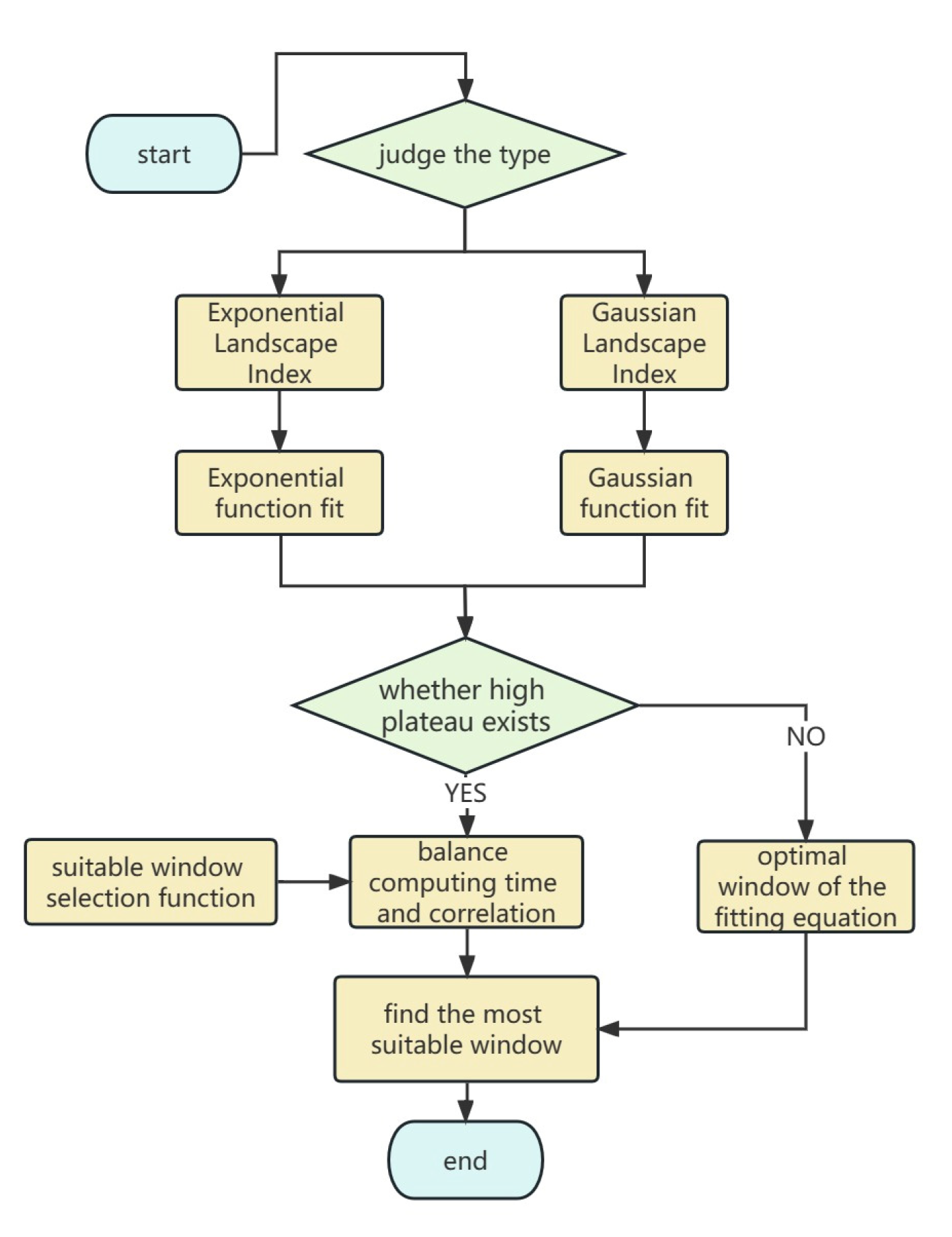
• We provide a method of selecting suitable window of correlation between landscape indices and land surface temperature. First, classify the landscape index into exponential landscape index or Gaussian landscape index. Second, use the fitting function corresponding to its type to fit and obtain the equation of the scale effect. Third, observe whether the curve has a high correlation plateau. If it has a high correlation plateau, we use suitable window selection function to calculate the suitable window. Otherwise, we calculate the optimal window by the fitting equation and the optimal window is the suitable window. The flow chart is shown in Figure 5.

The findings provide a basis for selecting the window size when studying the heat island effect and offer theoretical support for urban planners to reduce the heat island effect in their designs. Additionally, the results of this study can be used by local governments to make informed decisions about urban development and land use policies. Overall, this study has significant implications for urban planning and environmental management, and it highlights the importance of considering the scale effect when analyzing the relationship between landscape indices and land surface temperature.

4.2. Prospect

This study aimed to investigate the scale effect of the correlation between landscape index and land surface temperature using land use data from Nanjing. However, to generalize these findings, future work is necessary to verify them in other cities while taking into account the potential impact of regional climate and urban structure. It is important to note that while the scale effect determined by curve fitting provides valuable insights, it does not reveal the underlying mechanism. Therefore, future studies should focus on investigating the underlying mechanism to further our understanding of the relationship between landscape index and land surface temperature. The findings of this study could serve as a basis for selecting the optimal window size when studying the heat island effect, and provide theoretical support for urban planners to mitigate the heat island effect in their designs.

References

1. Zhang, H.; Luo, M.; Zhao, Y.; Lin, L.; Ge, E.; Yang, Y.; Ning, G.; Cong, J.; Zeng, Z.; Gui, K.; et al. HiTIC-Monthly: A Monthly High Spatial Resolution (1 km) Human Thermal Index Collection over China during 2003–2020. Earth Syst. Sci. Data 2023, 15, 359–381. [Google Scholar] [CrossRef]
2. Shi, X.; Xu, Y.; Wang, G.; Liu, Y.; Wei, X.; Hu, X. Spatiotemporal Variations in the Urban Heat Islands across the Coastal Cities in the Yangtze River Delta, China. Mar. Geod. 2021, 44, 467–484. [Google Scholar] [CrossRef]
3. Wei, C.; Chen, W.; Lu, Y.; Blaschke, T.; Peng, J.; Xue, D. Synergies between Urban Heat Island and Urban Heat Wave Effects in 9 Global Mega-Regions from 2003 to 2020. Remote Sens. 2021, 14, 70. [Google Scholar] [CrossRef]
4. Guo, Y.; Gasparrini, A.; Armstrong, B.G.; Tawatsupa, B.; Tobias, A.; Lavigne, E.; de Coelho, M.S.Z.S.; Pan, X.; Kim, H.; Hashizume, M.; et al. Heat Wave and Mortality: A Multicountry, Multicommunity Study. Env. Health Perspect. 2017, 125, 087006. [Google Scholar] [CrossRef] [PubMed]
5. Ma, H.-Y.; Li, H.-J.; Zhang, M.; Dong, X. Impact of Cropland Degradation in the Rural–Urban Fringe on Urban Heat Island and Heat Stress during Summer Heat Waves in the Yangtze River Delta. Adv. Clim. Change Res. 2022, 13, 240–250. [Google Scholar] [CrossRef]
6. Crandall, C.G.; González-Alonso, J. Cardiovascular function in the heat-stressed human. Acta Physiol. 2010, 199, 407–423. [Google Scholar] [CrossRef]
7. Robine, J.-M.; Cheung, S.L.K.; Le Roy, S.; Van Oyen, H.; Griffiths, C.; Michel, J.-P.; Herrmann, F.R. Death Toll Exceeded 70,000 in Europe during the Summer of 2003. Comptes Rendus Biol. 2008, 331, 171–178. [Google Scholar] [CrossRef]
8. Davis, R.E.; Knappenberger, P.C.; Novicoff, W.M.; Michaels, P.J. Decadal Changes in Summer Mortality in U.S. Cities. Int. J. Biometeorol. 2003, 47, 166–175. [Google Scholar] [CrossRef]
9. Hayashida, K.; Shimizu, K.; Yokota, H. Severe Heatwave in Japan. Acute Med. Surg. 2019, 6, 206–207. [Google Scholar] [CrossRef]
10. Tong, S.; Wang, X.Y.; Yu, W.; Chen, D.; Wang, X. The Impact of Heatwaves on Mortality in Australia: A Multicity Study. BMJ Open 2014, 4, e003579. [Google Scholar] [CrossRef]
11. Ma, W.; Zeng, W.; Zhou, M.; Wang, L.; Rutherford, S.; Lin, H.; Liu, T.; Zhang, Y.; Xiao, J.; Zhang, Y.; et al. The short-term effect of heat waves on mortality and its modifiers in China: An analysis from 66 communities. Environ. Int. 2015, 75, 103–109. [Google Scholar] [CrossRef] [PubMed]
12. Shukurov, I.S.; Le, M.T.; Shukurova, L.I.; Dmitrieva, A.D. Influence of the effect of the urban heat island on the cities sustainable development. UCA 2020, 10, 62–70. [Google Scholar] [CrossRef]
13. Wang, J.; Xiang, Z.; Wang, W.; Chang, W.; Wang, Y. Impacts of Strengthened Warming by Urban Heat Island on Carbon Sequestration of Urban Ecosystems in a Subtropical City of China. Urban Ecosyst. 2021, 24, 1165–1177. [Google Scholar] [CrossRef]
14. Jenerette, G.D.; Harlan, S.L.; Stefanov, W.L.; Martin, C.A. Ecosystem Services and Urban Heat Riskscape Moderation: Water, Green Spaces, and Social Inequality in Phoenix, USA. Ecol. Appl. 2011, 21, 2637–2651. [Google Scholar] [CrossRef]
15. Zhang, Z.; Zhang, J.; Liu, L.; Gong, J.; Li, J.; Kang, L. Spatial–Temporal Heterogeneity of Urbanization and Ecosystem Services in the Yellow River Basin. Sustainability 2023, 15, 3113. [Google Scholar] [CrossRef]
16. Tu, L.; Qin, Z.; Li, W.; Geng, J.; Yang, L.; Zhao, S.; Zhan, W.; Wang, F. Surface Urban Heat Island Effect and Its Relationship with Urban Expansion in Nanjing, China. J. Appl. Remote Sens. 2016, 10, 026037. [Google Scholar] [CrossRef]
17. Zhang, H.; Yin, Y.; An, H.; Lei, J.; Li, M.; Song, J.; Han, W. Surface Urban Heat Island and Its Relationship with Land Cover Change in Five Urban Agglomerations in China Based on GEE. Environ. Sci. Pollut. Res. 2022, 29, 82271–82285. [Google Scholar] [CrossRef] [PubMed]
18. Semenzato, P.; Bortolini, L. Urban Heat Island Mitigation and Urban Green Spaces: Testing a Model in the City of Padova (Italy). Land 2023, 12, 476. [Google Scholar] [CrossRef]
19. Njoku, E.A.; Tenenbaum, D.E. Quantitative Assessment of the Relationship between Land Use/Land Cover (LULC), Topographic Elevation and Land Surface Temperature (LST) in Ilorin, Nigeria. Remote Sens. Appl. Soc. Environ. 2022, 27, 100780. [Google Scholar] [CrossRef]
20. Zhou, H.; Wang, Q.; Zhu, N.; Li, Y.; Li, J.; Zhou, L.; Pei, Y.; Zhang, S. Optimization Methods of Urban Green Space Layout on Tropical Islands to Control Heat Island Effects. Energies 2022, 16, 368. [Google Scholar] [CrossRef]
21. Demissie, B.; Amsalu, A.; Tesfamariam, Z.; Nyssen, J.; Meaza, H.; Asfaha, T.G.; Zenebe, A.; Gregoretti, C.; Van Eetvelde, V. Landscape Changes in the Semi-Closed Raya Agricultural Graben Floor of Northern Ethiopia. Earth Syst. Environ. 2022, 6, 453–468. [Google Scholar] [CrossRef]
22. He, H.S.; DeZonia, B.E.; Mladenoff, D.J. An Aggregation Index (AI) to Quantify Spatial Patterns of Landscapes. Landsc. Ecol. 2000, 1, 591–601. [Google Scholar] [CrossRef]
23. Dušek, R.; Popelková, R. Theoretical View of the Shannon Index in the Evaluation of Landscape Diversity. AUC Geogr. 2017, 47, 5–13. [Google Scholar] [CrossRef]
24. Sun, D.; Dawson, R.; Li, H.; Wei, R.; Li, B. A landscape connectivity index for assessing desertification: A case study of Minqin County, China. Landsc. Ecol. 2007, 22, 531–543. [Google Scholar] [CrossRef]
25. Sun, Z.; Li, Z.; Zhong, J. Analysis of the Impact of Landscape Patterns on Urban Heat Islands: A Case Study of Chengdu, China. Int. J. Environ. Res. Public Health 2022, 19, 13297. [Google Scholar] [CrossRef]
26. Ye, H.; Li, Z.; Zhang, N.; Leng, X.; Meng, D.; Zheng, J.; Li, Y. Variations in the Effects of Landscape Patterns on the Urban Thermal Environment during Rapid Urbanization (1990–2020) in Megacities. Remote Sens. 2021, 13, 3415. [Google Scholar] [CrossRef]
27. Li, X.; Zhou, W.; Ouyang, Z. Relationship between Land Surface Temperature and Spatial Pattern of Greenspace: What Are the Effects of Spatial Resolution? Landsc. Urban Plan. 2013, 114, 1–8. [Google Scholar] [CrossRef]
28. Wu, J.; Shen, W.; Sun, W.; Tueller, P.T. Empirical patterns of the effects of changing scale on landscape metrics. Landsc. Ecol. 2002, 17, 761–782. [Google Scholar] [CrossRef]
29. Wu, Q.; Li, Z.; Yang, C.; Li, H.; Gong, L.; Guo, F. On the Scale Effect of Relationship Identification between Land Surface Temperature and 3D Landscape Pattern: The Application of Random Forest. Remote Sens. 2022, 14, 279. [Google Scholar] [CrossRef]
30. Yang, J.; Huang, X. The 30 m Annual Land Cover Dataset and Its Dynamics in China from 1990 to 2019. Earth Syst. Sci. Data 2021, 13, 3907–3925. [Google Scholar] [CrossRef]
31. Belgiu, M.; Drăguţ, L. Random forest in remote sensing: A review of applications and future directions. ISPRS J. Photogramm. Remote Sens. 2016, 114, 24–31. [Google Scholar] [CrossRef]
32. Cheng, J.; Meng, X.; Dong, S.; Liang, S. Generating the 30-m Land Surface Temperature Product over Continental China and USA from Landsat 5/7/8 Data. Sci. Remote Sens. 2021, 4, 100032. [Google Scholar] [CrossRef]
33. Verhoef, W.; Jia, L.; Xiao, Q.; Su, Z. Unified Optical-Thermal Four-Stream Radiative Transfer Theory for Homogeneous Vegetation Canopies. IEEE Trans. Geosci. Remote Sens. 2007, 45, 1808–1822. [Google Scholar] [CrossRef]
34. Jacquemoud, S. Inversion of the PROSPECT + SAIL canopy reflectance model from AVIRIS equivalent spectra: Theoretical study. Remote Sens. Environ. 1993, 44, 281–292. [Google Scholar] [CrossRef]
35. Yu, X.; Guo, X.; Wu, Z. Land Surface Temperature Retrieval from Landsat 8 TIRS—Comparison between Radiative Transfer Equation-Based Method, Split Window Algorithm and Single Channel Method. Remote Sens. 2014, 6, 9829–9852. [Google Scholar] [CrossRef]
36. Wang, M.; Zhang, Z.; Hu, T.; Wang, G.; He, G.; Zhang, Z.; Li, H.; Wu, Z.; Liu, X. An Efficient Framework for Producing Landsat-Based Land Surface Temperature Data Using Google Earth Engine. IEEE J. Sel. Top. Appl. Earth Obs. Remote Sens. 2020, 13, 4689–4701. [Google Scholar] [CrossRef]
37. Du, S.; Xiong, Z.; Wang, Y.; Guo, L. Quantifying the multilevel effects of landscape composition and configuration on land surface temperature. Remote Sens. Environ. 2016, 178, 84–92. [Google Scholar] [CrossRef]
38. Zhou, W.; Cao, F. Effects of Changing Spatial Extent on the Relationship between Urban Forest Patterns and Land Surface Temperature. Ecol. Indic. 2020, 109, 105778. [Google Scholar] [CrossRef]
39. Gage, E.A.; Cooper, D.J. Relationships between Landscape Pattern Metrics, Vertical Structure and Surface Urban Heat Island Formation in a Colorado Suburb. Urban Ecosyst. 2017, 20, 1229–1238. [Google Scholar] [CrossRef]
40. Li, J.; Zheng, X.; Zhang, C.; Deng, X.; Chen, Y. How to Evaluate the Dynamic Relevance between Landscape Pattern and Thermal Environment on Urban Agglomeration? Ecol. Indic. 2022, 138, 108795. [Google Scholar] [CrossRef]
41. Rakoto, P.Y.; Deilami, K.; Hurley, J.; Amati, M.; Sun, Q. (Chayn) Revisiting the Cooling Effects of Urban Greening: Planning Implications of Vegetation Types and Spatial Configuration. Urban For. Urban Green. 2021, 64, 127266. [Google Scholar] [CrossRef]
42. Connors, J.P.; Galletti, C.S.; Chow, W.T.L. Landscape Configuration and Urban Heat Island Effects: Assessing the Relationship between Landscape Characteristics and Land Surface Temperature in Phoenix, Arizona. Landsc. Ecol. 2013, 28, 271–283. [Google Scholar] [CrossRef]
43. Estoque, R.C.; Murayama, Y.; Myint, S.W. Effects of Landscape Composition and Pattern on Land Surface Temperature: An Urban Heat Island Study in the Megacities of Southeast Asia. Sci. Total Environ. 2017, 577, 349–359. [Google Scholar] [CrossRef] [PubMed]
44. Rhee, J.; Park, S.; Lu, Z. Relationship between Land Cover Patterns and Surface Temperature in Urban Areas. GISci. Remote Sens. 2014, 51, 521–536. [Google Scholar] [CrossRef]
Figure 1. The land use cover map of Nanjing.
Remotesensing 15 02131 g001
Figure 2. The figure of Pearson correlation coefficient. Note: AI: Aggregation Index, COHESION: Patch Cohesion Index, CONNECT: Connectance, CONTAG: Contagion, DIVISION: Landscape Division Index, MESH: Effective Mesh Size, MSIDI: Modified Simpson’s Diversity Index, PLADJ: Percentage of Like Adjacencies, SHDI: Shannon’s Diversity Index, TECI: Total Edge Contrast Index.
Remotesensing 15 02131 g002
Figure 3. Curve fitting of correlation coefficient between exponential landscape index and land surface temperature. The subplot contains the results of different landscape indices.
Remotesensing 15 02131 g003
Figure 4. Fitting results of correlation coefficient between Gaussian landscape index and land surface temperature. The subplot contains the results of different landscape indices.
Remotesensing 15 02131 g004
Figure 5. The flow chart of method of selecting suitable window.
Remotesensing 15 02131 g005