Abstract
Satellite imagery is the only feasible approach to annual monitoring and reporting on land cover change. Unfortunately, conventional pixel-based classification methods based on spectral response only (e.g., using random forests algorithms) have shown a lack of spatial and temporal stability due, for instance, to variability between individual pixels and changes in vegetation condition, respectively. Machine learning methods that consider spatial patterns in addition to reflectance can address some of these issues. In this study, a convolutional neural network (CNN) model, U-Net, was trained for a 500 km × 500 km region in southeast Australia using annual Landsat geomedian data for the relatively dry and wet years of 2018 and 2020, respectively. The label data for model training was an eight-class classification inferred from a static land-use map, enhanced using forest-extent mapping. Here, we wished to analyse the benefits of CNN-based land cover mapping and reporting over 34 years (1987–2020). We used the trained model to generate annual land cover maps for a 100 km × 100 km tile near the Australian Capital Territory. We developed innovative diagnostic methods to assess spatial and temporal stability, analysed how the CNN method differs from pixel-based mapping and compared it with two reference land cover products available for some years. Our U-Net CNN results showed better spatial and temporal stability with, respectively, overall accuracy of 89% verses 82% for reference pixel-based mapping, and 76% of pixels unchanged over 33 years. This gave a clearer insight into where and when land cover change occurred compared to reference mapping, where only 30% of pixels were conserved. Remaining issues include edge effects associated with the CNN method and a limited ability to distinguish some land cover types (e.g., broadacre crops vs. pasture). We conclude that the CNN model was better for understanding broad-scale land cover change, use in environmental accounting and natural resource management, whereas pixel-based approaches sometimes more accurately represented small-scale changes in land cover.
1. Introduction
According to Australia’s latest State of the Environment report [1], the country’s environment is generally in decline, with continued loss of natural capital across themes including land (e.g., native vegetation, soil, wetlands), biodiversity, inland waters, and marine environments. Land clearing has been an ongoing problem in Australia, despite Commonwealth legislation dedicated to environmental protection—the Environment Protection and Biodiversity Conservation Act 1999 and its predecessors—as well as legislation at state and territory levels. As much as 7.7 million hectares (an area larger than the island of Tasmania) of potential habitat and communities may have been cleared in the period 2000–2017 [2].
Monitoring land cover change is essential for existing and future policies to regulate native vegetation protection and land clearing, forest production, land and water conservation, and landscape carbon storage [3]. Satellite data provide a sound basis for understanding and mapping land cover change that is potentially internally consistent, repeatable over time, more economical and perhaps even more reliable than ground-based mapping [4]. Pixel-based machine learning methods based on spectral characteristics, such as random forests [5] and support vector machines [6], have been extensively used to turn remote-sensing images into land cover maps. In Australia, land cover mapping is available at 250 m and 30 m resolution using pixel-based methods [7,8,9]. The generation of more extensive time-series of land cover maps, with greater accuracy and reduced uncertainty has the potential to increase our understanding of Australia’s environmental change and land system processes [9].
In addition, deep learning methods have achieved promising results for many image-analysis tasks, including land use and land cover classification (e.g., [10,11,12]). A review published in 2019 [13] identified convolutional neural networks (CNNs) as the most common deep learning method for satellite image analysis in use at that time. CNNs find features in an image through a training process that generates neural network weights through an iterative gradient descent algorithm. CNNs generally consist of three building blocks: convolution and pooling layers (one to many), followed by a fully connected layer to determine the probable class. Since 2012, when they set new benchmarks for image recognition, CNNs have been successfully used for segmenting remote-sensing images to generate land cover and vegetation maps [14,15,16]. The median accuracy of land cover classifications from deep learning is generally higher than that from established classifiers such as random forests or support vector machines [13]. In the context of annual land cover change monitoring and reporting, it is even more problematic that pixel-based classifiers can show a lack of spatial and temporal stability, e.g., due to variability between individual pixels and changes in vegetation condition, respectively (e.g., [17,18,19,20]). Machine learning methods that consider spatial patterns in addition to spectral information, such as CNNs, may address some of these issues.
Studies of the evolution of land cover over time using remote-sensing data [21] typically exploit spectral, spatial, or temporal data to build models using multiple acquisitions within a single year (e.g., [22,23]) or multiple years (e.g., [24]) using a satellite image time series. Methods generally employ supervised classification to assign a class to a pixel based on a model trained to compare input data to label data [25,26]. Unfortunately, in the Australian context, a general lack of high-resolution label data for the years before 2018 prevents the temporal component from being easily incorporated in model building.
The following hypotheses motivated the work described here:
- CNN models can produce land cover maps that are spatially and temporally more consistent than those generated using pixel-based methods; and
- CNN models are sufficiently robust to map, quantify and interpret changes in major land cover classes over decadal time scales.
In this study, we wished to specifically analyse the spatial and temporal stability of CNN-based land cover mapping over 34 years of Landsat imagery (1987–2020). We applied a pre-trained U-Net CNN model and developed innovative diagnostic methods to assess spatial and temporal stability. We used the diagnostics to quantitatively and qualitatively analyse how the CNN method differs from pixel-based mapping, which is the main contribution of this study. The results were compared to the recently released annual Digital Earth Australia (DEA) Land Cover product for 1988–2020 [27] generated using pixel-based classifiers, as well as the annual global ESRI Land Cover product for 2017–2021 [28] that was created using a U-Net CNN model trained from scratch, but which received limited or no specific training data for Australian conditions.
2. Materials and Methods
The study area (Figure 1) was an area of approximately 500 km × 500 km (~400 million pixels) in south-eastern Australia for which annual Landsat geomedian data at 25 m resolution [29] was available in GDA94/Australian Albers projection (EPSG:3577) from Geoscience Australia. Annual geomedian data are pixel composites generated using a high-dimensional statistic called the ‘geometric median’, which enables the production of a representative cloud-free annual composite image [30]. Pixel-based compositing methods have been used to exploit large data volumes on annual or seasonal time scales to create representative images [31] as inputs to machine learning model development.
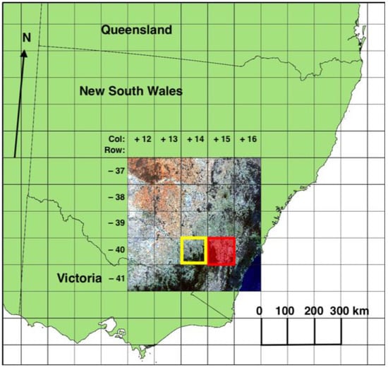
Figure 1.
Study area (2018 Landsat 8 geomedian true colour RGB), test tile +14, −40 (yellow box). Canberra tile +15, −40 (red box) used for application of U-Net CNN model for the period 1987–2020. Projection: GDA94/Australian Albers (EPSG:3577).
Figure 2 shows the modelling and analysis workflow of the study, documenting the analysis steps and how they relate to sections in the results.
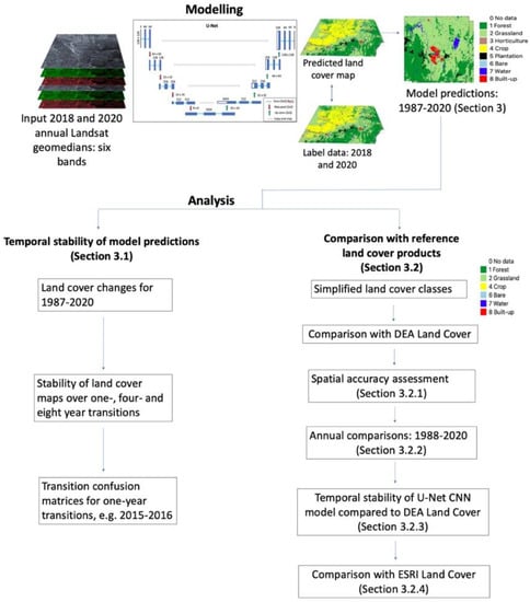
Figure 2.
Modelling and analysis workflow of study.
A U-Net CNN model [32] was built using input Landsat annual geomedian v2 data [29] for 2018 (a dry year) and 2020 (a wet year). Label data for model development was a simple eight-class land cover classification (Bare, Built-up, Crop, Forest, Grassland, Horticulture, Plantation, Water plus an unknown No data class) derived from reference land-use mapping [33,34], that was enhanced using forest-extent mapping [35], using the approach described in [17].
The U-Net CNN model, with ResNet50 encoder and transfer learning of ImageNet weights, was trained using Landsat annual geomedian six-band data (Blue, Green, Red, NIR, SWIR1, SWIR2) for 2018 and 2020 and corresponding label data. The study area (19,968 × 19,968 pixels) was broken into 24,336 non-overlapping 128 × 128 pixel patches for 2018 and 2020. Patches over the ocean (694) were discarded and the land-based tiles for each year (23,642) were split into training, validation, and test sets (Table 1).

Table 1.
Dataset splits used for model development. Test set from tile +14, −40 (Figure 1).
The models were trained using the Adam optimiser [36] with a batch size of eight and an initial learning rate of 0.0001 determined through multiple iterations of these hyperparameters to identify the most performant configuration. Each model was trained for up to 80 epochs, ten epochs at a time, to generate a ‘best model’ with the highest validation accuracy and weighted-mean F1 score, using the methods and software as described in [17]. The learning rate was automatically reduced after ten epochs if validation accuracy failed to improve as model training approached the optimal solution. Imbalanced class distributions were managed using the dice and focal loss functions following [37]:
Total_loss = Dice_loss + (1 × Focal_loss)
To reduce risk of overfitting and increase the dataset size, data augmentation was applied using the fast augmentation library Albumentations [38]. Transformations included a random selection of image blurring and sharpening, gaussian noise addition, cropping, flipping, mirroring, and affine and perspective changes. Models were built for ten epochs and the results were examined. Those with the highest validation accuracy were saved and examined for the test area (tile +14, −40 in the Geoscience Australia Landsat tiling system, see Figure 1) to determine through visual inspection the degree of match between predicted land cover and label data.
The best CNN model was then applied to 34 years (1987–2020) of Landsat annual geomedian data for a tile of 100 km × 100 km (16 million pixels; one million hectares) surrounding the city of Canberra (tile +15, −40, Figure 1) to generate land cover maps for each year. The input geomedian reflectances were derived from Landsat 5 for 1987–1999 and 2003–2011, Landsat 7 for 2000–2002 and 2012, and Landsat 8 for 2013–2020.
Here, our focus was on the spatial and temporal stability of annual U-Net CNN model results compared to pixel-based classifiers and reference land cover products. Specifically, the following analyses were carried out on U-Net CNN model results for 1987–2020 using a combination of Python programs, the open-source Geographic Information System QGIS, and spreadsheets in Microsoft Excel:
- 3.
- Investigation of the spatial and temporal stability of land cover classes between years using methods defining model transition probabilities (cf., [39]);
- 4.
- Comparison to the DEA Land Cover product for 1988–2020 [8,40] created using pixel-based methods (including Random Forests) using the same annual geomedian data; and
- 5.
- Comparison to the ESRI Land Cover product, a global Sentinel-2 10-m Land Use/Land Cover product for 2017–2021 [28] created using a U-Net model trained from scratch but not specifically developed or evaluated for Australia.
The authors developed a model transition probability classification for one-year, four-year and eight-year transitions (Table 2), to assist in understanding transitions that are likely to be real versus those that may be artefacts of the model itself. The transition probability classification was developed by the authors through an extensive discussion, consensus, and agreement process. The classification categorised changes as either as Possible (P), Unlikely (U) or Implausible (I). The assessment has an element of subjectivity but the authors quickly reached consensus on transition probabilities. Overall change statistics for one, four and eight-year land cover transitions were generated considering their likelihood. One-year transitions were examined in detail to infer the most likely reasons for the results.
Table 2.
Matrix showing one (first letter), four (second letter) and eight-year (third letter) transitions, respectively, of mapped land cover and their likelihood: Possible (P), unlikely (U) or implausible (I) changes. No change transitions on diagonal (left blank).
The DEA Land Cover product was chosen for comparison for several reasons: it was generated from the same annual Landsat geomedian data we used as input; it covered a similar range of years (1988–2020); and, importantly, it uses more conventional pixel-based machine learning methods, including Random Forests. The DEA Land Cover product was first converted to a simple land cover classification similar to ours (Table 3). The DEA Land Cover product uses the FAO Land Cover Classification System [41]. Simplifying its Level-4 classification enabled comparison to our land cover classes for each year from 1988–2020. It was not possible to separate the DEA class Natural Terrestrial Vegetated: Woody into our Forest and Plantation classes. Similarly, the DEA class Cultivated Terrestrial Vegetated covers both our Horticulture and Crop classes. Therefore, we amalgamated those classes for the comparison, yielding a simplified classification of six classes (plus No data for the remainder, see Table 3).
Table 3.
Class correspondence table for DEA Land Cover level 4 to U-Net CNN land cover.
Using simplified label data for 2018 as a reference, confusion matrices comparing the 2018 simplified CNN and DEA results were generated to assess their spatial classification accuracy. Metrics used were overall accuracy (OA) [42], Kappa coefficient [43], and class weighted-mean F1 scores as described in [17].
Confusion matrices comparing the simplified CNN and DEA maps were also generated for every year from 1988–2020 to assess the degree of correspondence and summary statistics were calculated. The simplified CNN maps for 2018 and 2020 were used to calculate fractions for class weighted-mean value calculations.
Our CNN results were also compared to the ESRI Land Cover product, which was generated using Sentinel-2 data. Although this dataset only overlaps with our data for four years (2017–2020), the comparison was of interest because the ESRI product uses a similar U-Net methodology to map land cover, albeit at a higher resolution and using a globally trained model. The ESRI product produces a set of nine simple land cover classes (Table 4) applied globally using a U-Net CNN model. The ESRI data were reprojected to the same Australian Albers projection and then resampled to 25-m resolution to match our CNN maps. Classes were also mapped to a common simplified land cover classification (Table 4). Our CNN mapping results were directly compared to the ESRI Land Cover data and statistics were generated for the four years of overlap (2017–2020) between the two products.
Table 4.
Class correspondence table for ESRI Land Cover to U-Net CNN land cover.
3. Results
For the study area, the best CNN model, generated after 40 epochs, had an overall accuracy of 80% and a weighted-mean F1 score for all classes of 77%. The 2018 model output for the study area (Figure 3c) compares well visually with label data (Figure 3b) and the Landsat geomedian true colour RGB image (Figure 3a). At this regional scale, the model results reflect several features (e.g., forest, water, grassland) that are also recognisable in the Landsat geomedian input.
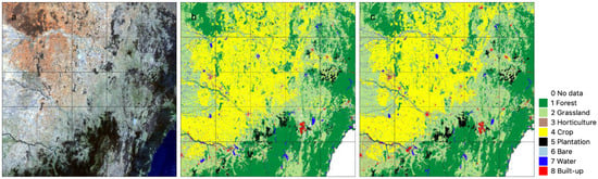
Figure 3.
Input Landsat data as True colour RGB (a); label/reference data (b); and U-Net CNN model results (c) for 2018 and study area (~500 km × 500 km).
The CNN model was used to generate yearly land cover maps for 1987–2020 (34 years) for the Canberra tile (~100 km × 100 km, Figure 1). Land cover is dominated by forest in the southwest and southeast, with smaller built-up areas associated with the central urban area of Canberra, plantation forest to the west and east of the city, water over Lake Burrinjuck in the north-west and Lake George in the central east, with the rest of the tile being largely made up of grassland (Figure 4). Crops are cultivated in this region, but the CNN was not effective in detecting this class, nor the horticulture (mainly vineyards) that occurs to the north of Canberra. Some broad-scale changes over the full period are detectable, including the gradual increase of the Canberra urban area (Built-up) and loss of plantations due to bushfires in 2003 to the west of Canberra. Figure 4c and Table 5 show the increase in Forest of ~55,000 hectares (16%) and decrease in Grassland of ~79,000 hectares (14%) over 34 years, as well as a significant increase in Built-up, reflecting the growth of Canberra, of ~20,000 hectares (82%). Large increases in crop and horticulture are from a low base and are not considered to be reliable.
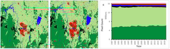
Figure 4.
U-Net CNN model results for 1987 (a); and 2020 (b); and land cover class distribution (c) (legend as for Figure 3).
Table 5.
Extent of predicted land cover classes for 1987 and 2020 showing changes.
3.1. Temporal Stability of U-Net CNN Model Predictions
One-year, four-year (e.g., 1987–1991, 1991–1995, etc.) and eight-year (e.g., 1987–1995, 1995–2003, etc.) transitions were analysed, and summary statistics were calculated. One-year transitions resulted in fewer changes in land cover, with an average 95.4% of pixels showing no change between consecutive years (Table 6). This compares with an average 93.4% and 91.8% of pixels showing no change for the four-year and eight-year transitions, respectively. Regarding transitions deemed possible, the results show an average increase from 2.3% via 3.2% to 3.8% of pixels for one-, four-, and eight-year transitions, respectively. For transitions deemed unlikely, one- and four-year changes are 0.1% before increasing to 4% for eight-year transitions. In contrast, implausible transitions showed an increase from 2.1% for one-year to 3.2% for four-year transitions before a decrease to 0.3% for eight-year transitions. This reversal probably reflects the change in the transition likelihood classification (Table 2). Some transitions in land cover considered implausible over four years were considered merely unlikely over eight years, mainly relating to the conversion of Grassland to Forest, Forest to Plantation, and Plantation to Forest. The standard deviations of mean transitions are below 1.1%, suggesting that average changes between years are relatively stable over time (Table 6).
Table 6.
Summary statistics for one, four and eight-year transitions of CNN model results for 1987–2020.
Of the one-year transitions, the pair of years with the least change was 2015–2016 (Figure 5). Some minor differences between 2015 and 2016 occur over Lake George (red box) and in Plantation, Forest and Built-up classes. Table 7 shows a transition matrix for 2015–2016, highlighting transition categories: no change, possible, unlikely and implausible changes. Of the implausible changes, the most common ones are from Built-up to Grassland (0.25%), Forest to Plantation (0.21%), Plantation to Forest (0.17%) and Grassland to Forest (0.16%) which largely appear to be edge effects associated with class boundaries (Figure 5 and Supplementary Materials Table S1).
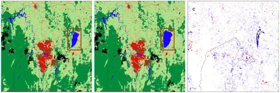
Figure 5.
U-Net CNN model results for 2015 (a); and 2016 (b) (legend as for Figure 3); and change map (c). Highlighting differences: No change (white), possible (blue), unlikely (yellow), and implausible (red).
Table 7.
Transition matrix showing the number of pixels with no (bold), possible (plain text), unlikely (italics) and implausible (underlined) land cover change from 2015 to 2016. Note that the CNN method did not map any cropland.
3.2. Comparison of U-Net CNN Model Predictions with Reference Land Cover Products
Simplifying the land cover classification to six classes provided a means to compare model results with two reference land cover products: DEA Land Cover (1988–2020) and ESRI Land Cover (2017–2021).
Simplified U-Net CNN model results for 2018 were compared to Landsat input data, simplified reference label data and DEA Land Cover in Figure 6. 2018 had the closest match (Figure S1) between CNN model results (Figure 6c) and DEA Land Cover (Figure 6d), also for a year where high-resolution label data was available (Figure 6b).
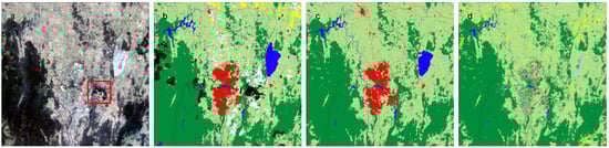
Figure 6.
2018 Landsat geomedian (true colour RGB) input (a), simplified label data (b), U-Net CNN model (c) and DEA Land Cover (d) (b–d use the simplified classification of six land cover classes).
3.2.1. Spatial Accuracy Assessment
A spatial accuracy assessment based on confusion matrices was undertaken by comparing U-Net CNN and DEA Land Cover results, respectively, to 2018 label data as the reference. Compared to the DEA Land Cover product, the CNN results had higher overall accuracy (89 vs. 82%), Kappa (82 vs. 69%), and class weighted-mean F1 score (89 vs. 81%) (Table 8 and Table 9). For the Forest class, results are similar with a producer’s accuracy (how often real features in the landscape are shown in the classified map) of 91% vs. 92%, while for other classes the U-Net CNN shows better producer’s accuracy then DEA Land Cover (Grassland 94% vs. 87%; Bare 63% vs. 25%; Water 61% vs. 15%; Built-up 87% vs. 13%) with the exception being the Crop class which was not detected well by either method (0.4% vs. 14%).
Table 8.
Simplified U-Net CNN model vs. simplified label data for 2018. OA = 89%, Kappa = 82% and weighted-mean F1 = 89%. Excludes No data pixels.
Table 9.
Simplified DEA Land Cover vs. simplified label data for 2018. OA = 82%, Kappa = 69% and weighted-mean F1 = 81%. Excludes No data pixels.
3.2.2. Annual Comparisons: 1988–2020
To better understand model results over time, confusion matrices comparing the simplified CNN to the DEA mapping were generated for 33 years (1988–2020), and overall accuracy (OA), Kappa and class weighted-mean F1 scores were calculated for each year using DEA as the reference (Supplementary Figure S1 and Table 10). The overall accuracy of these yearly comparisons ranged from about 50–86% and weighted-mean F1 from 56–85% (Table 10). Kappa values ranged from 33–75%, translating to fair agreement (>20% and ≤40%) for three years, moderate agreement (>40% and ≤60%) for 19 years and substantial agreement (>60% and ≤80%) for 11 years following the classification proposed by [44].
Table 10.
Summary statistics for Figure S1—Variation in OA, Kappa and weighted-mean F1 for 1998–2020.
The best correlation between the simplified U-Net CNN model and simplified DEA Land Cover was obtained for 2018 (OA 86%, Kappa 75% and class weighted-mean F1 score 84%), while the worst correlation was for 2020 (OA 50%, Kappa 33% and class weighted-mean F1 score 56%). The confusion matrices for these comparisons are provided in Tables S2 and S3, respectively.
Substantial spatial differences between our CNN and the DEA mapping (Figure 6c,d) occur in the urban area of Canberra, Lake George and small areas of crop and forest, mostly north and east of the city. The U-Net CNN model in 2018 identified a smaller extent of the Crop class in this tile compared to DEA Land Cover and neither result appears to effectively represent this class as referenced in the label data (Figure 6b). Though DEA Land Cover is a closer match for this class, its Crop extent is largely not spatially coincident with the label data. Differences in the Forest class between the U-Net CNN model and DEA Land Cover are minor and limited to class boundary or edge effects, as well as a difference associated with an area of partially cleared plantation Forest (red box in Figure 6a) immediately east of the Canberra urban area which is not completely detected in either result. A mixture of the classes Forest, Grassland, Bare, Built-up and Crop can be seen across the urban area in the simplified DEA Land Cover, with an abundance of isolated pixels producing a grainy visual effect (Figure 6d). For Lake George, the U-Net CNN model classifies this area as Water, although in 2018 this area would have been largely dry, whereas DEA Land Cover, arguably more realistically, classifies the area as mainly Bare and Grassland, with some small amounts of Water, but also Forest and Crop, which are considered unlikely to occur in this area.
Visually there is good spatial correspondence between simplified DEA Land Cover classes and U-Net CNN model results, particularly for the Forest, Water and Grassland classes (Figure 6). DEA Land Cover classes represented by each U-Net CNN model class are shown for Forest/Plantation (Figure 7), Grassland (Figure 8a) and Built-up (Figure 8b). For the U-Net CNN model Forest and Plantation classes, the vast majority of pixels from the simplified DEA Land Cover map are the class Natural Terrestrial Vegetated: Woody (Figure 7), with a gradual increase in the classes with trees from 1988–2020, and a correlation between trends in the respective classes of R2 = 0.47 (Figure 9a). In contrast, the agreement is not as close for the U-Net CNN model class Grassland. As expected, the majority of CNN grassland corresponds to the DEA class Natural Terrestrial Vegetated: Herbaceous (Figure 8a). However, there was also a considerable proportion (5–70%) of Cultivated Terrestrial Vegetated: Herbaceous and a smaller proportion (2–18%) of Natural Terrestrial Vegetated: Woody.
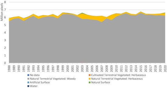
Figure 7.
DEA Land Cover classes that correspond to the U-Net CNN model Forest and Plantation classes.
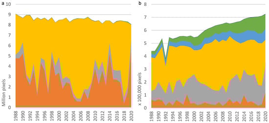
Figure 8.
DEA Land Cover classes that correspond to the U-Net CNN model Grassland class (a); and Built-up class (b). Legend as for Figure 7.
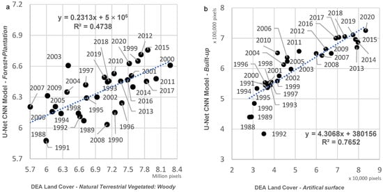
Figure 9.
Relationship between DEA Land Cover and U-Net CNN model for Natural Terrestrial Vegetation: Woody vs. Forest + Plantation (a) and Artificial Surface vs. Built-up (b). Other classes are less well correlated.
For the U-Net CNN model Built-up class, the expected Artificial Surface class occupied only 6–12% of pixels (Figure 8b). Instead, the most common corresponding DEA Land Cover classes were Natural Terrestrial Vegetated: Herbaceous and Natural Terrestrial Vegetated: Woody. Despite the lower number of pixels, the trend in the DEA Land Cover Artificial Surface class correlated reasonably well with the U-Net CNN model Built-up class (R2 = 0.77; Figure 9b). Urban growth is more monotonic for U-Net CNN Built-up with increases recorded for 28 years (88%) from 1988–2020 compared to 21 years (66%) for DEA Land Cover’s Artificial Surface. Comparing temporal trends, the U-Net CNN model appeared to produce anomalous results for 1992 (Figure 8b).
The U-Net CNN model did not identify the Crop class accurately and instances of crop across land cover maps are relatively few, e.g., for 1987, 2020 (Figure 4). In contrast, the DEA Land Cover product mapped large extents of Cultivated Terrestrial Vegetated: Herbaceous (Crop) (e.g., Supplementary Figure S2). However, examination of transitions of this class suggests the extent is overestimated and has considerable temporal instability between years, as shown in Figure 10 for 1993–1995 (similar patterns were seen for other periods, e.g., 1996–1998). Field observations by the authors suggest that these rapid changes are not realistic.
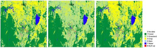
Figure 10.
Temporal instability of Crop unit (yellow), derived from Cultivated Terrestrial Vegetated: Herbaceous, in simplified DEA Land Cover for 1993–1995.
The spatial extent of the Built-up class (Figure 11) in the simplified U-Net CNN model closely reflects the urban areas visible in the Landsat RGB image with a few areas of over-classification and unclear boundaries (e.g., the industrial area indicated by a yellow rectangle in Figure 11c). Roads are generally correctly classified by the U-Net CNN model as Built-up, whereas the pixel-based methods used to generate DEA Land Cover often classify roads as Forest or Grassland (possibly reflecting roadside vegetation), e.g., Figure 11b, or as Crop, e.g., Figure 11c.
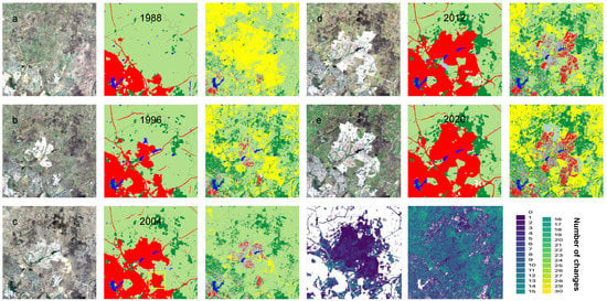
Figure 11.
Gungahlin area in the north of Canberra showing the growth of urban areas, with (a–e) for every eighth year from 1988 to 2020, triplets showing the Landsat geomedian RGB True Colour composite (left), and six-class simplified land cover maps (for legend see Figure 10) from our CNN mapping (centre) and the DEA Land Cover product (right). Area is ~14 km × 14 km centred on 35.18°S, 149.12°E. (f) number of class transitions (legend at right) over 1988–2020 for our CNN model (left) and the DEA Land Cover product (right).
Newly developed urban areas in the DEA Land Cover (right image of three, Figure 11) are predominantly classified as Built-up or Bare, as might be expected. Older urban areas visible to the southwest in the 1988 image and subsequent years show many pixels classified as Forest, Grassland and even Crop, perhaps reflecting the low-density, vegetation-rich character of Canberra’s established suburbs.
Forest areas are generally defined well spatially in both our CNN results and DEA mapping. In the Grassland and Crop areas (Figure 11), DEA Land Cover shows the previously mentioned frequent change between these classes, which is unlikely to be accurate. There is cropping in these areas, but such large variations over a one-year (Figure 10) to eight-year (Figure 11) time scale do not occur in the authors’ observation.
Figure 12 shows a comparison of land cover classes defined by the U-Net CNN model and DEA Land Cover for 1988–2020 for the area from Figure 11. The U-Net CNN model shows more stability between years (except for the anomalous year 1992) and gradual changes to land cover classes appear closely matched to features (e.g., built-up and forest areas) visible in Landsat images. In contrast, DEA Land Cover shows large changes in the Grassland and Crop classes between years and more variability in the Forest class.
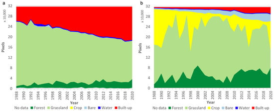
Figure 12.
Distribution of land cover classes for 1988–2020 for simplified U-Net CNN model (a); and simplified DEA Land Cover (b) for Gungahlin area in Figure 11.
3.2.3. Temporal Stability of U-Net CNN Model Compared to DEA Land Cover
Characterising how often individual pixels change between consecutive years (1988–2020) and mapping results provides a measure of temporal stability (Figure 13). If a pixel changes every year, there would be a total of 32 changes across the 33 years (inclusive) from 1988 to 2020. Other than Lake George, forested and water areas in both the U-Net CNN model and DEA Land Cover maps are well conserved through the 33 years with no or few changes recorded (white areas in the southwest, southeast, and northwest, Figure 13). Lake George shows many changes in both the CNN and DEA mapping; this is not unexpected, given that it is a shallow ephemeral lake with highly variable extent that is regularly completely dry. For the U-Net CNN model, the urban areas of Canberra (central area) are conserved (white areas) but not in the DEA mapping.
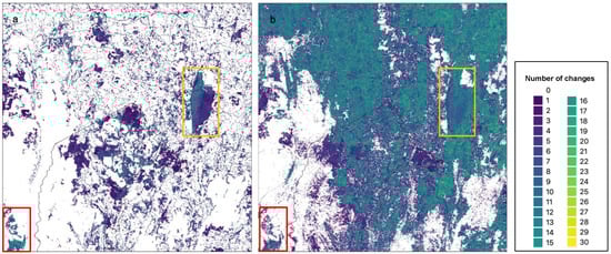
Figure 13.
Total number of changes for simplified U-Net CNN model (a); maximum = 29, and simplified DEA Land Cover (b). Maximum = 30. Lake George (orange box) and southwest of tile (red box) highlighted.
In our CNN results, changes are often associated with class boundaries (e.g., red box in Figure 13a), as well as linear effects associated predominantly with roads. In the DEA mapping, changes are mostly associated with the coverage of the Crop and Grassland classes (e.g., Figure 10), and the urban area where there is a grainy, ‘salt and pepper’ mix of classes that changes through time (Figure 13b).
Judging by the distribution of the number of class transitions for 1988–2020, the U-Net CNN model is more temporarily stable than DEA Land Cover (Figure 14). Almost 76% of pixels in the CNN mapping do not change class over this period, whereas only 30% of the pixels for DEA Land Cover are unchanged. The number of pixels experiencing 1–4 changes over the period is similar for both maps, but from five changes on, the U-Net CNN model has significantly fewer pixel changes than DEA Land Cover. For example, the U-Net CNN model has about 11% of pixels showing more than four changes over 33 years, whereas for the DEA Land Cover, 55% of pixels have more than four changes in this period.
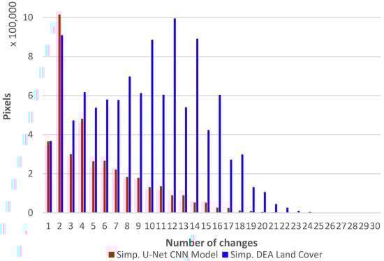
Figure 14.
Pixel changes for 1988–2020 for simplified U-Net CNN model and simplified DEA Land Cover.
3.2.4. Comparison of U-Net CNN Model Predictions with ESRI Land Cover
A comparison of the simplified U-Net CNN model result for 2017 and simplified ESRI Land Cover is provided in Supplementary Figure S3. The ESRI map (Figure S3b) showed more Built-up in rural areas, as well as more Crop and Grassland than the simplified U-Net CNN model (Figure S3a). The two maps do show temporal correlation (Figure S4). It is reiterated that both results were obtained using U-Net CNN models, although the algorithms were separately trained and used input imagery from different sources and resolution (Landsat vs. Sentinel-2). Temporal correlation (Figure S4) between the changing extent of the built-up (R2 = 1.0) and forest (R2 = 0.91) classes in the mapping by our and the ESRI algorithm was considerable, though only four years overlap between datasets were available (2017–2020). Correlation for other classes is lower, e.g., R2 = 0.38 for Water and R2 = 0.20 for Crop.
4. Discussion
The accuracy of label data affects the quality of the trained classifier. In a previous study [17], 800 randomly selected pixels (100 per land cover class) were examined to validate the label data used here using high-resolution imagery. Their validation suggested that the trained model is, in fact, slightly more accurate than the label data, with the ‘real’ CNN model OA and mean F1 values at least 4–5% higher than those calculated using the label data as a reference. They concluded that the CNN model generally distinguished major land cover classes correctly despite inaccuracies in the label data. Here, our focus was on the spatial and temporal stability of our U-Net CNN model and its ability to map changes in major land cover classes over time.
4.1. Spatial and Temporal Stability
Confusion matrices (Table 8 and Table 9) illustrate the differences in spatially determined accuracy and other metrics of the CNN model result and DEA Land Cover for 2018 compared to reference label data. The CNN exhibits greater spatial stability with overall accuracy, Kappa and weighted-mean F1 being 7–13% higher than the pixel-based algorithm and per class producer’s accuracy (recall) substantially higher for the Built-up, Water, Bare and Grassland classes. However, some of these differences, particularly for the Built-up and Water classes, are likely related to a capability mismatch between the broader scale of target label data with its homogeneous classes, and pixel-based methods which operate at a finer scale, as further discussed later in this section.
The U-Net CNN model results showed good temporal stability, with 95%, 93% and 92% of pixels unchanged, on average, over one, four and eight-year periods (Table 6); with this stability mapped spatially as total changes by pixel for years 1988–2020 in Figure 13a. Some issues in land cover maps generated by the model were detected, evident from the occurrence of implausible land cover transitions. Lake George is an ephemeral shallow lake that during drier periods is partially bare or covered with sparse vegetation or grassland. Hence, the changing model interpretation of this area as Water, Bare or Grassland class is explicable. However, other classes, such as Forest (e.g., 2015 in Figure 5a), are unlikely to be correct. It was further found that the 1992 map was anomalous, with insufficient Plantation and Built-up in the model result. We interpret that this was due to the anomalous geomedian reflectance images for this year. This implies that the CNN model relies on spectral information in addition to spatial patterns.
Examination of the Canberra urban area helps with understanding the spatial stability of results (Figure 8b), in terms of both the simplified U-Net CNN model (e.g., Figure S2b) and simplified DEA Land Cover (e.g., Figure S2c). Canberra, locally known as the ‘bush capital’, includes considerable forest and grassland within the urban green space and remnant vegetation, with a total canopy cover of about 23% within its urban footprint according to a 2020 LiDAR study [45]. This helps to explain the DEA Land Cover results, which focus on a pixel-level determination of land cover. This pixel-based classification may be correct but fails to detect the broader scale spatial definition of urban area, which was better identified by the U-Net CNN model. To a degree, this difference appears to relate to a contrast in the effective scale of mapping between pixel-based and CNN mapping. Making use of spatial context, the CNN creates mapping units that are greater than one pixel (i.e., 625 m2). In contrast, the DEA method does not consider spatial context and strictly classifies individual pixels. These methodological differences cause implicit differences in scale and definition that need not always be inherently inconsistent. Following the example given here, there can be smaller areas of vegetation within the urban area that the CNN correctly identifies as part of the Built-up area while also correctly identified by the DEA product as Terrestrial Vegetation. Combining the pixel-based and CNN-based classification results could help to reconcile much of this ambiguity and create a new level of mapping sophistication (e.g., Terrestrial Vegetation within Built-up areas).
Studies of the effects of spatial resolution and internal land cover class variability on classification accuracy (e.g., [46,47]) show that using lower spatial resolution imagery or smoothing or texture filters can lead to increased classification accuracy. Similarly, object-based classification approaches [48,49] can result in more generalised and visually acceptable depictions of land cover classes than pixel-based methods. Broadly, these results appear to be analogous to what was observed in this study concerning the contrast in the effective scale of mapping between pixel-based methods (operating at higher resolution) and the CNN (aggregating pixels to create larger mapping units). This is particularly true for land cover classes comprising different surface covers, such as urban areas.
Linear features such as roads are an interesting case as the road surface itself is often less than 25 m wide and, therefore, may not be mapped by pixel-based methods or else mapped as Forest or Grassland (reflecting roadside vegetation). In contrast to pixel-based approaches, the U-Net CNN model is better at correctly mapping these features as Built-up using label data and the signature of roadside verges and parallel tree rows in Landsat input images. The CNN model’s ability to detect rivers and roads correctly seems in part to rely on the label data, which includes a cadastral representation of these linear features and these typically contain publicly owned river corridors and road easements, respectively. By contrast, the DEA mapping relies entirely on the interpretation of the Landsat geomedian image, which can lead to misclassification, perhaps due to the presence of riparian or roadside vegetation, respectively (e.g., Figure 11). The use of pre- or post-processing might improve these results for pixel-based methods.
Nonetheless, the U-Net CNN showed some issues of its own for linear features and unit boundaries. As noted by [13], CNN are prone to producing rounded edges and blunted corners for mapped land cover classes and sometimes show an undesirable loss of object detail. Some studies have reduced these issues through modifications to the CNN model methodology. An interesting area for future work would be the addition of the temporal dimension to model building through the application of a temporal CNN [50] or by using transformers [51] in combination with the U-Net CNN (e.g., [52]). The latter can potentially improve, among others, the extraction of linear features such as roads [53].
4.2. Mapping Changes in Major Land Cover Classes over Time
Eight land cover classes were mapped annually for the Canberra tile for the 34 years of 1987–2020. Pixel statistics on the distribution of land cover classes over time were generated (Figure 4c and Figure 12a). These results generally show systematic and explicable changes in major land cover classes. They include a gradual increase in Built-up area, mainly reflecting the urbanisation of Canberra, an increase in Forest and a decline in Grassland over the same period. In terms of the Water class, results are more variable, e.g., with lower rainfall during the Millennium Drought (1997–2009) visible in the extent of that class. Plantation extent gradually increased until 2003, when bushfires west of the city removed approximately 38% of this class before a gradual recovery over the remaining years to 2020. Results for the Bare class are variable with no apparent pattern and may reflect real changes in clearing and urban development over time. Results for the Horticulture and Crop classes are not considered reliable, however. For these classes, the results are highly variable during 1987–2020, which may indicate that the CNN was not able to detect these land cover classes accurately from the Landsat input data. Because the imagery represents a single annual geomedian, it cannot capture changes in reflectance associated with the seasonal phenology of cultivated vegetation. Sub-annual reflectance information might help improve the distinction between Grassland, Horticulture, and Crop.
Summarising, our U-Net CNN model proved useful for broad-scale land cover mapping over time, with several advantages over pixel-based mapping methods. U-Net CNN models operate at a broader spatial scale producing more stable and consistent results for the segmentation of images into land cover units, generally without ‘salt and pepper’ issues, as also noted by [10,20]. By contrast, the use of DEA Land Cover for accurate estimation of total urban area or grassland/crop and their change over time did not appear to be feasible. Both methods each had their own strengths and weaknesses, but overall, a CNN rather than pixel-based mapping approach might be needed to produce sufficient spatial and temporal stability for applications such as environmental accounting [54,55] and other land cover monitoring activities to support natural resource management (e.g., [56]).
5. Conclusions
A U-Net CNN model was applied to annual Landsat geomedian input data for 1987–2020 to generate a series of land cover maps that are more stable and consistent over several decades compared to pixel-based approaches. Although the CNN had some issues with linear features, rounded class boundaries and a reduction in object detail that is not always desirable, the U-Net CNN model results showed better spatial coherence than results generated using pixel-based methods such as random forests and produced a more spatially and temporally consistent interpretation of the landscape at the regional scale. The U-Net CNN model operated at a coarser, more aggregated level than the individual pixel, allowing it to detect contextual information to generate a more stable spatial distribution of land cover classes through time, whereas pixel-based methods are better able to detect fine-scale variations within inhomogeneous classes, e.g., vegetation within urban areas. The U-Net CNN used for land cover mapping also appeared to be more temporally stable than pixel-based mapping, with fewer class changes (24% vs. 70% of pixels) over 33 years (1988–2020).
In summary, the U-Net CNN model appears to be capable of broad-scale land cover mapping over time, with several advantages over pixel-based mapping methods. The spatial transferability of the methods described here to other regions within Australia needs to be tested and is a subject for future research.
Supplementary Materials
The following supporting information can be downloaded at: https://www.mdpi.com/article/10.3390/rs15082132/s1, Table S1: 2015–2016 transition statistics: No change (bold), possible change (plain text), and unlikely (italics) and implausible (underlined) changes showing class transitions; Figure S1: 1998–2020 simplified CNN vs. DEA mapping confusion matrix statistics; Table S2: Simplified U-Net CNN model vs. simplified DEA Land Cover for 2018. OA = 86%, Kappa = 75% and weighted-mean F1 = 84%. Excludes No data pixels; Table S3: Simplified U-Net CNN model vs. simplified DEA Land Cover for 2020. OA = 50%, Kappa = 33% and weighted-mean F1 = 56%. Excludes No data pixels; Figure S2: Simplified U-Net CNN model (b) and simplified DEA Land Cover (c) and input Landsat data as True colour RGB (a) for Canberra urban area in 2013; Figure S3: 2017 simplified U-Net CNN Model (a), simplified ESRI Land Cover (b) and differences (c). Difference map shows ESRI Land Cover classes where they are different to the U-Net CNN model; Figure S4: Relationship between ESRI Land Cover and U-Net CNN model for Built area vs. Built-up (a) and Trees vs. Forest + Plantation (b). Other classes are less well correlated.
Author Contributions
Conceptualisation, investigation, methodology, software, writing—original draft, writing—review and editing, T.B.; supervision, visualisation, writing—review and editing, A.V.D.; supervision, writing—review and editing, R.T. All authors have read and agreed to the published version of the manuscript.
Funding
This research was supported by an Australian Government Research Training Program (RTP) Scholarship.
Data Availability Statement
The data presented in this study are available on request from the corresponding author.
Conflicts of Interest
The authors declare that they have no known competing financial interests or personal relationships that could have appeared to influence the work reported in this paper.
References
- Cresswell, I.D.; Janke, T.; Johnston, E.L. Australia State of the Environment 2021: Overview; Independent Report to the Australian Government Minister for the Environment; Commonwealth of Australia: Canberra, Australia, 2021. [Google Scholar] [CrossRef]
- Ward, M.S.; Simmonds, J.S.; Reside, A.E.; Watson, J.E.M.; Rhodes, J.R.; Possingham, H.P.; Trezise, J.; Fletcher, R.; File, L.; Taylor, M. Lots of Loss with Little Scrutiny: The Attrition of Habitat Critical for Threatened Species in Australia. Conserv. Sci Pract. 2019, 1, e117. [Google Scholar] [CrossRef]
- Thackway, R. (Ed.) Land Use in Australia: Past, Present and Future; ANU Press: Canberra, Australia, 2018; Available online: https://press.anu.edu.au/publications/land-use-australia (accessed on 1 November 2022).
- Defries, R.S.; Townshend, J.R.G. Global Land Cover Characterization from Satellite Data: From Research to Operational Implementation? GCTE/LUCC Research Review. Glob. Ecol. Biogeogr. 1999, 8, 367–379. [Google Scholar] [CrossRef]
- Breiman, L. Random Forests. Mach. Learn. 2001, 45, 5–32. [Google Scholar] [CrossRef]
- Huang, C.; Davis, L.S.; Townshend, J.R.G. An Assessment of Support Vector Machines for Land Cover Classification. Int. J. Remote Sens. 2002, 23, 725–749. [Google Scholar] [CrossRef]
- Lymburner, L.; Tan, P.; Mueller, N.; Thackway, R.; Lewis, A.; Thankappan, M.; Randall, L.; Islam, A.; Senarath, U. The National Dynamic Land Cover Dataset 2011; Geoscience Australia, ACT: Symonston, Australia, 2011; pp. 3297–3300. [Google Scholar]
- Owers, C.J.; Lucas, R.M.; Clewley, D.; Tissott, B.; Chua, S.M.T.; Hunt, G.; Mueller, N.; Planque, C.; Punalekar, S.M.; Bunting, P.; et al. Operational Continental-Scale Land Cover Mapping of Australia Using the Open Data Cube. Int. J. Digit. Earth 2022, 15, 1715–1737. [Google Scholar] [CrossRef]
- Calderón-Loor, M.; Hadjikakou, M.; Bryan, B.A. High-Resolution Wall-to-Wall Land-Cover Mapping and Land Change Assessment for Australia from 1985 to 2015. Remote Sens. Environ. 2021, 252, 112148. [Google Scholar] [CrossRef]
- Zhang, W.; Tang, P.; Zhao, L. Fast and Accurate Land-Cover Classification on Medium-Resolution Remote-Sensing Images Using Segmentation Models. Int. J. Remote Sens. 2021, 42, 3277–3301. [Google Scholar] [CrossRef]
- González-Vélez, J.C.; Martinez-Vargas, J.D.; Torres-Madronero, M.C. Land Cover Classification Using CNN and Semantic Segmentation: A Case of Study in Antioquia, Colombia. In Smart Technologies, Systems and Applications; Narváez, F.R., Proaño, J., Morillo, P., Vallejo, D., González Montoya, D., Díaz, G.M., Eds.; Communications in Computer and Information Science; Springer International Publishing: Cham, Switzerland, 2022; Volume 1532, pp. 306–317. ISBN 978-3-030-99169-2. [Google Scholar]
- Ulmas, P.; Liiv, I. Segmentation of Satellite Imagery using U-Net Models for Land Cover Classification. arXiv 2020, arXiv:2003.02899. [Google Scholar]
- Ma, L.; Liu, Y.; Zhang, X.; Ye, Y.; Yin, G.; Johnson, B.A. Deep Learning in Remote Sensing Applications: A Meta-Analysis and Review. ISPRS J. Photogramm. Remote Sens. 2019, 152, 166–177. [Google Scholar] [CrossRef]
- Zhu, X.X.; Tuia, D.; Mou, L.; Xia, G.-S.; Zhang, L.; Xu, F.; Fraundorfer, F. Deep Learning in Remote Sensing: A Comprehensive Review and List of Resources. IEEE Geosci. Remote Sens. Mag. 2017, 5, 8–36. [Google Scholar] [CrossRef]
- Hoeser, T.; Kuenzer, C. Object Detection and Image Segmentation with Deep Learning on Earth Observation Data: A Review-Part I: Evolution and Recent Trends. Remote Sens. 2020, 12, 1667. [Google Scholar] [CrossRef]
- Kattenborn, T.; Leitloff, J.; Schiefer, F.; Hinz, S. Review on Convolutional Neural Networks (CNN) in vegetation remote sensing. ISPRS J. Photogramm. Remote Sens. 2021, 173, 24–49. [Google Scholar] [CrossRef]
- Boston, T.; Van Dijk, A.; Larraondo, P.R.; Thackway, R. Comparing CNNs and Random Forests for Landsat Image Segmentation Trained on a Large Proxy Land Cover Dataset. Remote Sens. 2022, 14, 3396. [Google Scholar] [CrossRef]
- Blaschke, T.; Lang, S.; Lorup, E.; Strobl, J.; Zeil, P. Object-Oriented Image Processing in an Integrated GIS/Remote Sensing Environment and Perspectives for Environmental Applications. Environ. Inf. Plan. Politics Public 2000, 2, 555–570. [Google Scholar]
- Phiri, D.; Morgenroth, J. Developments in Landsat Land Cover Classification Methods: A Review. Remote Sens. 2017, 9, 967. [Google Scholar] [CrossRef]
- Zhang, X.; Han, L.; Han, L.; Zhu, L. How Well Do Deep Learning-Based Methods for Land Cover Classification and Object Detection Perform on High Resolution Remote Sensing Imagery? Remote Sens. 2020, 12, 417. [Google Scholar] [CrossRef]
- Gómez, C.; White, J.C.; Wulder, M.A. Optical Remotely Sensed Time Series Data for Land Cover Classification: A Review. ISPRS J. Photogramm. Remote Sens. 2016, 116, 55–72. [Google Scholar] [CrossRef]
- Pelletier, C.; Valero, S.; Inglada, J.; Champion, N.; Dedieu, G. Assessing the Robustness of Random Forests to Map Land Cover with High Resolution Satellite Image Time Series over Large Areas. Remote Sens. Environ. 2016, 187, 156–168. [Google Scholar] [CrossRef]
- Stoian, A.; Poulain, V.; Inglada, J.; Poughon, V.; Derksen, D. Land Cover Maps Production with High Resolution Satellite Image Time Series and Convolutional Neural Networks: Adaptations and Limits for Operational Systems. Remote Sens. 2019, 11, 1986. [Google Scholar] [CrossRef]
- Khiali, L.; Ndiath, M.; Alleaume, S.; Ienco, D.; Ose, K.; Teisseire, M. Detection of Spatio-Temporal Evolutions on Multi-Annual Satellite Image Time Series: A Clustering Based Approach. Int. J. Appl. Earth Obs. Geoinf. 2019, 74, 103–119. [Google Scholar] [CrossRef]
- Hansen, M.C.; Defries, R.S.; Townshend, J.R.G.; Sohlberg, R. Global Land Cover Classification at 1 Km Spatial Resolution Using a Classification Tree Approach. Int. J. Remote Sens. 2000, 21, 1331–1364. [Google Scholar] [CrossRef]
- Townshend, J.R.; Masek, J.G.; Huang, C.; Vermote, E.F.; Gao, F.; Channan, S.; Sexton, J.O.; Feng, M.; Narasimhan, R.; Kim, D.; et al. Global Characterization and Monitoring of Forest Cover Using Landsat Data: Opportunities and Challenges. Int. J. Digit. Earth 2012, 5, 373–397. [Google Scholar] [CrossRef]
- Geoscience Australia. Digital Earth Australia-Public Data-Land Cover (Landsat) v1.0.0. 2021. Available online: https://cmi.ga.gov.au/data-products/dea/607/dea-land-cover-landsat (accessed on 1 November 2022).
- Karra, K.; Kontgis, C.; Statman-Weil, Z.; Mazzariello, J.C.; Mathis, M.; Brumby, S.P. Global Land Use/Land Cover with Sentinel 2 and Deep Learning. In Proceedings of the 2021 IEEE International Geoscience and Remote Sensing Symposium IGARSS, Brussels, Belgium, 11 July 2021; pp. 4704–4707. [Google Scholar] [CrossRef]
- Geoscience Australia. Digital Earth Australia-Public Data-Surface Reflectance 25m Geomedian v2.1.0. 2019. Available online: https://data.dea.ga.gov.au/?prefix=geomedian-australia/v2.1.0/ (accessed on 1 November 2022).
- Roberts, D.; Mueller, N.; Mcintyre, A. High-Dimensional Pixel Composites From Earth Observation Time Series. IEEE Trans. Geosci. Remote Sens. 2017, 55, 6254–6264. [Google Scholar] [CrossRef]
- White, J.C.; Wulder, M.A.; Hobart, G.W.; Luther, J.E.; Hermosilla, T.; Griffiths, P.; Coops, N.C.; Hall, R.J.; Hostert, P.; Dyk, A.; et al. Pixel-Based Image Compositing for Large-Area Dense Time Series Applications and Science. Can. J. Remote Sens. 2014, 40, 192–212. [Google Scholar] [CrossRef]
- Ronneberger, O.; Fischer, P.; Brox, T. U-Net: Convolutional Networks for Biomedical Image Segmentation. In Medical Image Computing and Computer-Assisted Intervention—MICCAI 2015. MICCAI 2015; Navab, N., Hornegger, J., Wells, W., Frangi, A., Eds.; Lecture Notes in Computer Science; Springer: Cham, Switzerland, 2015; Volume 9351. [Google Scholar] [CrossRef]
- ABARES. Catchment Scale Land Use of Australia—Update December 2018. 2019. Available online: https://www.agriculture.gov.au/abares/aclump/land-use/catchment-scale-land-use-of-australia-update-december-2018 (accessed on 1 November 2022).
- ABARES. Catchment Scale Land Use of Australia—Update December 2020. 2021. Available online: https://www.agriculture.gov.au/abares/aclump/catchment-scale-land-use-of-australia-update-december-2020 (accessed on 1 November 2022).
- ABARES. Forests of Australia (2018). 2019. Available online: https://www.agriculture.gov.au/abares/forestsaustralia/forest-data-maps-and-tools/spatial-data/forest-cover (accessed on 1 November 2022).
- Kingma, D.P.; Ba, J. Adam: A Method for Stochastic Optimization. In Proceedings of the 3rd International Conference on Learning Representations, ICLR 2015, San Diego, CA, USA, 7–9 May 2015. [Google Scholar]
- Zhu, W.; Huang, Y.; Zeng, L.; Chen, X.; Liu, Y.; Qian, Z.; Du, N.; Fan, W.; Xie, X. AnatomyNet: Deep learning for fast and fully automated whole-volume segmentation of head and neck anatomy. Med. Phys. 2019, 46, 576–589. [Google Scholar] [CrossRef] [PubMed]
- Buslaev, A.; Iglovikov, V.I.; Khvedchenya, E.; Parinov, A.; Druzhinin, M.; Kalinin, A.A. Albumentations: Fast and Flexible Image Augmentations. Information 2020, 11, 125. [Google Scholar] [CrossRef]
- Yuan, F.; Sawaya, K.E.; Loeffelholz, B.C.; Bauer, M.E. Land Cover Classification and Change Analysis of the Twin Cities (Minnesota) Metropolitan Area by Multitemporal Landsat Remote Sensing. Remote Sens. Environ. 2005, 98, 317–328. [Google Scholar] [CrossRef]
- Lucas, R.; Mueller, N.; Siggins, A.; Owers, C.; Clewley, D.; Bunting, P.; Kooymans, C.; Tissott, B.; Lewis, B.; Lymburner, L.; et al. Land Cover Mapping Using Digital Earth Australia. Data 2019, 4, 143. [Google Scholar] [CrossRef]
- Di Gregorio, A.; Jansen, L.J.M. Land Cover Classification System: Classification Concepts and User Manual: LCCS, Software version 2; 8 Environment and Natural Resources Series; Food and Agriculture Organization of the United Nations: Rome, Italy, 2005; ISBN 978-92-5-105327-0. [Google Scholar]
- Metz, C.E. Basic Principles of ROC Analysis. Semin. Nucl. Med. 1978, 8, 283–298. [Google Scholar] [CrossRef]
- Cohen, J. A Coefficient of Agreement for Nominal Scales. Educ. Psychol. Meas. 1960, 20, 37–46. [Google Scholar] [CrossRef]
- Landis, J.R.; Koch, G.G. The Measurement of Observer Agreement for Categorical Data. Biometrics 1977, 33, 159. [Google Scholar] [CrossRef]
- ACT Government. Canberra’s Tree Canopy Continues to Grow. 2021. Available online: https://www.cmtedd.act.gov.au/open_government/inform/act_government_media_releases/chris-steel-mla-media-releases/2021/canberras-tree-canopy-continues-to-grow (accessed on 1 November 2022).
- Cushnie, J.L. The Interactive Effect of Spatial Resolution and Degree of Internal Variability within Land-Cover Types on Classification Accuracies. Int. J. Remote Sens. 1987, 8, 15–29. [Google Scholar] [CrossRef]
- Aplin, P.; Atkinson, P.M.; Curran, P.J. Fine Spatial Resolution Simulated Satellite Sensor Imagery for Land Cover Mapping in the United Kingdom. Remote Sens. Environ. 1999, 68, 206–216. [Google Scholar] [CrossRef]
- Blaschke, T. Object Based Image Analysis for Remote Sensing. ISPRS J. Photogramm. Remote Sens. 2010, 65, 2–16. [Google Scholar] [CrossRef]
- Duro, D.C.; Franklin, S.E.; Dubé, M.G. A Comparison of Pixel-Based and Object-Based Image Analysis with Selected Machine Learning Algorithms for the Classification of Agricultural Landscapes Using SPOT-5 HRG Imagery. Remote Sens. Environ. 2012, 118, 259–272. [Google Scholar] [CrossRef]
- Pelletier, C.; Webb, G.; Petitjean, F. Temporal Convolutional Neural Network for the Classification of Satellite Image Time Series. Remote Sens. 2019, 11, 523. [Google Scholar] [CrossRef]
- Vaswani, A.; Shazeer, N.; Parmar, N.; Uszkoreit, J.; Jones, L.; Gomez, A.N.; Kaiser, Ł.; Polosukhin, I. Attention Is All You Need. In Proceedings of the Advances in Neural Information Processing Systems (NIPS 2017); Guyon, I., Luxburg, U.V., Bengio, S., Wallach, H., Fergus, R., Vishwanathan, S., Garnett, R., Eds.; Curran Associates, Inc.: Red Hook, NY, USA, 2017; Volume 30, Available online: https://proceedings.neurips.cc/paper/2017/file/3f5ee243547dee91fbd053c1c4a845aa-Paper.pdf (accessed on 6 March 2023).
- Garnot, V.S.F.; Landrieu, L. Panoptic Segmentation of Satellite Image Time Series with Convolutional Temporal Attention Networks. In Proceedings of the 2021 IEEE/CVF International Conference on Computer Vision (ICCV), Montreal, QC, Canada, 11–17 October 2021; pp. 4852–4861. [Google Scholar] [CrossRef]
- Yao, J.; Jin, S. Multi-Category Segmentation of Sentinel-2 Images Based on the Swin UNet Method. Remote Sens. 2022, 14, 3382. [Google Scholar] [CrossRef]
- United Nations et al. System of Environmental-Economic Accounting—Ecosystem Accounting (SEEA EA). 2021. Available online: https://seea.un.org/ecosystem-accounting (accessed on 1 November 2022).
- Edens, B.; Maes, J.; Hein, L.; Obst, C.; Siikamaki, J.; Schenau, S.; Javorsek, M.; Chow, J.; Chan, J.Y.; Steurer, A.; et al. Establishing the SEEA Ecosystem Accounting as a Global Standard. Ecosyst. Serv. 2022, 54, 101413. [Google Scholar] [CrossRef]
- Australian Bureau of Statistics. National Land Cover Account, ABS. 2022. Available online: https://www.abs.gov.au/statistics/environment/environmental-management/national-land-cover-account/latest-release (accessed on 1 November 2022).
Disclaimer/Publisher’s Note: The statements, opinions and data contained in all publications are solely those of the individual author(s) and contributor(s) and not of MDPI and/or the editor(s). MDPI and/or the editor(s) disclaim responsibility for any injury to people or property resulting from any ideas, methods, instructions or products referred to in the content. |
© 2023 by the authors. Licensee MDPI, Basel, Switzerland. This article is an open access article distributed under the terms and conditions of the Creative Commons Attribution (CC BY) license (https://creativecommons.org/licenses/by/4.0/).