Article

Lagged Linkage between the Kara–Barents Sea Ice and Early Summer Rainfall in Eastern China in Chinese CMIP6 Models

Key Laboratory of Meteorological Disaster of Ministry of Education, ILCEC, Collaborative Innovation Center on Forecast and Evaluation of Meteorological Disasters, Nanjing University of Information Science and Technology, Nanjing 210044, China
*
Author to whom correspondence should be addressed.
Remote Sens. 2023, 15(8), 2111; https://doi.org/10.3390/rs15082111
Submission received: 8 March 2023 / Revised: 1 April 2023 / Accepted: 14 April 2023 / Published: 17 April 2023

Abstract

:
The lagged relationship between Kara–Barents sea ice and summer precipitation in eastern China is evaluated for Chinese models participating in phase 6 of the Coupled Model Intercomparison Project (CMIP6). A previous study revealed a dipole rainfall structure in eastern China related to winter Arctic sea ice variability. Almost all Chinese CMIP6 models reproduce the variability and climatology of the sea ice in most of the Arctic well except the transition regions with evident biases. Further, all Chinese CMIP6 models successfully simulate the decreasing trend for the Kara–Barents sea ice. The dipole centers located in the Yangtze–Huai River Valley (YHRV) and South China (SC) related to Kara–Barents sea ice variability are simulated with different degrees of success. The anomalous dipole rainfall structure related to the winter Kara–Barents sea ice variability can roughly be reproduced by two models, while other models reproduce a shifted rainfall anomaly pattern or with the sign reversed. The possible delayed influence of sea ice forcing on early summer precipitation in China is established via three possible processes: the long memory of ice, the long-lasting stratospheric anomalies triggered by winter sea ice forcing, and the downward impact of the stratosphere as the mediator. Most Chinese models can simulate the negative Northern Hemisphere Annular Mode (NAM) phase in early winter but fail to reproduce the reversal of the stratospheric anomalies to a positive NAM pattern in spring and early summer. Most models underestimate the downward impact from the stratosphere to the troposphere. This implies that the stratospheric pathway is essential to mediate the winter sea ice forcing and rainfall in early summer over China for CMIP6 models.

1. Introduction

Sea ice is a crucial component in the Arctic marine system, whose impact on global weather and climate change is observable. Arctic sea ice variability can prevent momentum, heat, and moisture exchanges between air and ocean and modulate surface albedo [1,2,3]. Both the thickness and coverage of ice have shown a dramatic declining trend over the past decades [4,5,6]. Sea ice melting weakens westerlies at the upper level and drives the jet stream to move northward, increasing the risk of heat waves in the summer [7]. Therefore, special attention should be paid to polar sea ice variability, which has deep implications for the forecasts of climate and weather extremes in the Northern Hemisphere [8].
Recent studies have shown that atmospheric teleconnection across mid-to-high latitudes can bridge the remote impact of sea ice on extreme weather and climate in Eurasia and North America [9,10]. The blocking circulation and planetary waves can be amplified due to the reduced temperature gradient between high and midlatitudes with the ice loss [11,12,13,14]. Other researchers have also documented that winter atmospheric circulation may be affected by autumn–winter sea ice forcing [15,16,17]. For instance, sea ice variabilities across Greenland in winter could affect the summer atmospheric circulation and therefore lead to rainfall changes in Eurasia [9,13,18]. Anomalous sea ice loss in the Barents–Kara–Laptev Seas in autumn may lead to extreme coldness in Eurasia in the following winter [19]. Recent studies have noted the pathways by which stratospheric anomalies can affect global climate and weather and proposed the influence of gravity waves [20,21,22]. Some studies have also revealed the stratospheric changes associated with ice change [23,24,25], which could further trigger a downward influence on regional rainfall and atmospheric circulation. For instance, Yang et al. [25] indicated that the NAM response in the stratosphere is reversed in spring following sea ice loss in the Kara–Barents Seas, which is possibly due to the fact that the suppressed waves in winter tend to break out in the following months and contribute to a weaker polar vortex. This reversal of the stratospheric circulation anomalies from early winter to spring has also been noticed by Hu et al. [26]. Other studies have emphasized that the anomalous ice forcing is followed by a strengthened troposphere–stratosphere interaction [27,28].
Recent studies have explored the possible connections between rainfall anomalies in the Northern Hemisphere and Arctic ice [29,30]. The Bering and Okhotsk sea ice loss in spring tends to be followed by the southward extension of Arctic cold air, contributing to a wetter pattern in southeastern China [31]. The increase (decrease) of Arctic ice in spring may exert a drier (wetter) pattern in South China and a wetter (drier) pattern in northeast China [32]. The Barents sea ice variability in June can lead to a triple rainfall structure across eastern China in August [33]. The potential connections between other climate elements and sea ice anomalies are also examined, including surface temperature and haze pollution [34,35].
Several studies have revealed that the Kara–Barents seas are a key region with large sea ice variability [36,37,38]. The cold extremes across northern continents are often accompanied by Kara–Barents sea ice decline [16,38]. The weakening of the winter Siberian high may also be relevant to the growth of autumn Kara–Barents sea ice, which can, in turn, weaken the East Asian winter monsoon and lead to increased temperatures in China [39]. Many studies have indicated that summer climate elements in northeast Asia are also affected by the Barents sea ice [33,40,41], especially rainfall. For instance, Barents sea ice anomalies may affect Eurasian atmospheric circulation and the precipitation distribution of East China in the late spring and early summer [42]. Kara–Barents sea ice variability could also influence the cyclonic circulation over Siberia and the Kara–Barents seas, which further cause heatwave events in North China and create favorable conditions for precipitation over southern North China [43]. Han et al. revealed that the Kara–Barents sea ice variability in early spring could affect midsummer rainfall in northeast China, which is important for local agriculture production [44].
Compared with the former phase, the Coupled Model Intercomparison Project Phase 6 (CMIP6) has been improved in several aspects, such as the resolution and the physical processes [45,46]. A previous study documented that the multimodel ensemble mean can well represent the trend and the annual cycle of sea ice [47]. However, the possible teleconnection related to the sea ice variability has not been assessed for CMIP6 models. Yang et al. [25] established a robust linkage between Kara–Barents sea ice variability and June precipitation over eastern China. The aim of this study is to fully assess the ability of Chinese CMIP6 models to capture the lagged sea ice–rainfall relationship between Arctic sea ice and rainfall in China with an expectation of providing a first-hand reference for Chinese modeling groups to further improve the overall performance of the models.
The article is constructed as follows: Section 2 describes the datasets and methods used. Section 3 presents the simulation results for sea ice, rainfall, and their relationship using Chinese CMIP6 models. The physical processes are also analyzed in this section, including the sea ice persistency, the atmospheric changes from the troposphere to the stratosphere related to Kara–Barents sea ice variability, and the possible downward impact from the stratosphere. Finally, the discussion and conclusions are presented in Section 4.

2. Materials and Methods

2.1. Baseline Data

Several datasets are used as a baseline to assess the results of the sea ice–precipitation relationship in ten Chinese CMIP6 models. The monthly data of sea ice concentration (SIC) is obtained from the UK Met Office Hadley Centre (MOHC), which has a horizontal resolution of 1° × 1° (latitude × longitude) and spans from 1870 to the present [48]. The sea ice concentration (SIC) refers to the proportion of the grid area covered by sea ice. The most recent modern reanalysis from ECMWF (ERA5) [49] is also adopted in this study, which has a finer horizontal resolution (0.25° × 0.25°, latitude × longitude) at 37 pressure levels. We downloaded this dataset at a 1.5° × 1.5° resolution from 1979 to 2020 for easy reading and storage. Variables used include meridional winds, zonal winds, and geopotential (divided by 9.8 to obtain geopotential heights) at 37 pressure levels. In addition, the precipitation observations are provided by the Climate Prediction Center Merged Analysis of Precipitation (CMAP) with a 2.5° × 2.5° resolution from 1979 to the near present [50]. Note that the relationship between the circulation and SIC during 1979–2020 is nearly identical to that during 1950–2014, and only the results using the data from 1979–2020 are shown to keep consistent with the time span of the available CMAP data.

2.2. CMIP6 Models and Outputs

Ten Chinese CMIP6 models with historical run data available are used to examine the performance of the state-of-the-art models in simulating the sea ice–rainfall relationship and the associated processes. An introduction to the ten Chinese models is briefly listed in Table 1. The full name, institution, resolution, sea ice, and land surface for each CMIP6 model are also provided in Table 1. The historical experiment is driven by observed historical forcings, which range from 1850 to 2014. We extracted the 1950–2014 period from the first historical run to denote the present climate conditions. The analyzed variables include zonal winds, meridional winds, geopotential heights, precipitation, and SIC.

2.3. Methods

The lead/lag regression and composite are employed to examine the potential linkage between winter ice and early summer precipitation in China after both the seasonal cycle and the trend in each calendar month are removed from each dataset for each variable. Several indices are calculated as follows. The area-averaged SIC over 20–90°E and 65–85°N (i.e., SIC weighted by the cosine of the latitude) refers to the Kara–Barents sea ice index. Rainfall in two subregions of China is significantly correlated with the Kara–Barents SIC. One of the regions is the Yangtze–Huai River Valley (YHRV, 110–122°E, 28–36°N), and the other is South China (SC, 105–122°E, 22–28°N).

3. Results

3.1. Climatology of SIC and Rainfall in CMIP6 Models

3.1.1. Climatology of the SIC in the Arctic

The mean state of the ice in November–December in observations and 10 CMIP6 models are shown in Figure 1. Yang et al. [25] have shown a larger SIC variability in November–December than in other months, so we focus on those two months. In observations, full sea ice is distributed in most of the Arctic Ocean (Figure 1k). Most Chinese CMIP6 models (excluding CIESM) successfully simulate the distribution of Arctic SIC (Figure 1a–j). A previous study has suggested that SIC biases are mainly situated in the Okhotsk, Bering, Barents, and East Greenland Seas [51]. The Kara–Barents SIC in FIO-ESM2-0, NESM3, and TaiESM1 is well simulated, while six models (Figure 1a–d,f,g) overestimate the Kara–Barents SIC. In contrast, the SIC is not reasonably simulated in CIESM.
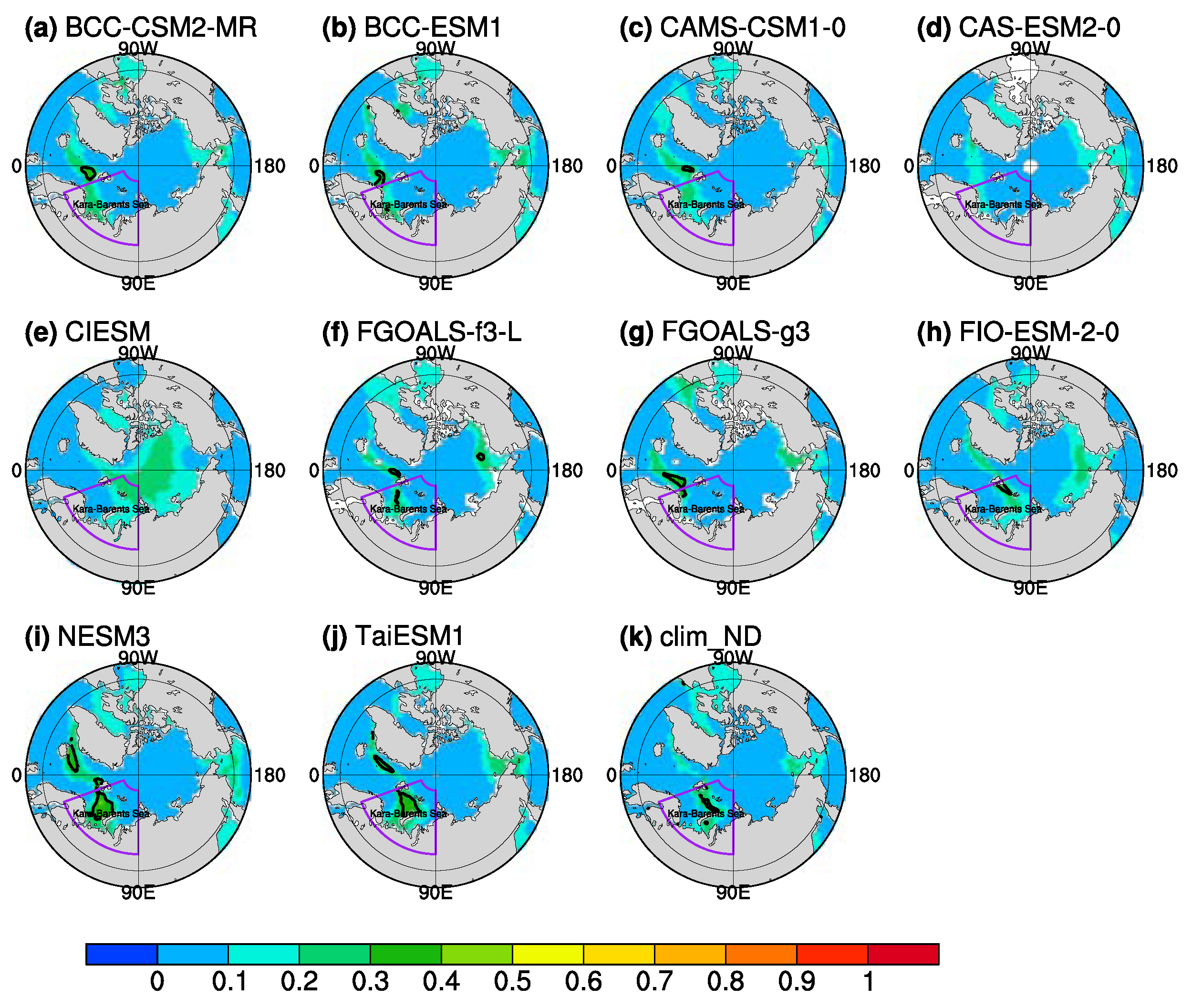
Figure 2 shows the variability of Arctic SIC in November and December for Chinese CMIP6 models and observations. In observations, the regions covered with full ice show little SIC variability, and the large variability usually appears in the transition regions (Figure 2k). We also noted that the Kara–Barents Seas show the largest SIC variability in the subpolar regions. The Chinese CMIP6 models simulate the distribution of SIC variability with different degrees of success. The maximum centers and amplitudes of SIC in FGOALS-f3-L, FIO-ESM2-20, NESM3, and TaiESM1 are fairly similar to observations (Figure 2f,h–j). The SIC variability centers are biased equatorward in four models (Figure 2a–d). The maximum SIC variability in FGOALS-g3 is biased westward (Figure 2g), while the SIC variability in CIESM is illusively large in most of the Arctic Ocean.

3.1.2. Climatology of Early Summer Rainfall

Guo et al. [52] showed that the East Asia summer monsoon (EASM) is significantly related to the Arctic SIC in spring. It is necessary to test the Chinese CMIP6 models’ performance in simulating East Asia rainfall before the lagged relation between the Arctic SIC and rainfall is established. Figure 3 shows the variability and the climatology of June rainfall in East Asia for the CMIP6 models and CMAP observations. The total monthly precipitation declines from southeast to northwest, and two centers are present in CMAP: YHRV and SC (Figure 3k). The precipitation variability also decreases from south to north, and two variability centers are evident. The Chinese models reasonably simulate the general distribution of the climatology and variability of June rainfall in China (Figure 3a–j). Half of the Chinese models overestimate the June precipitation in both of the two key regions (Figure 3a–c,f,g). Three models reproduce the June precipitation in the south well but underestimate the monthly precipitation in the north (CAS-ESM2-0, NESM3, and TaiESM1; Figure 3d,i,j). Further, the Chinese CMIP6 models also show a similar rainfall variability distribution to the CMAP observations. Namely, the maximum rainfall variability is mainly located over the coastal regions and the ocean, and the rainfall variability declines from the south to the north.
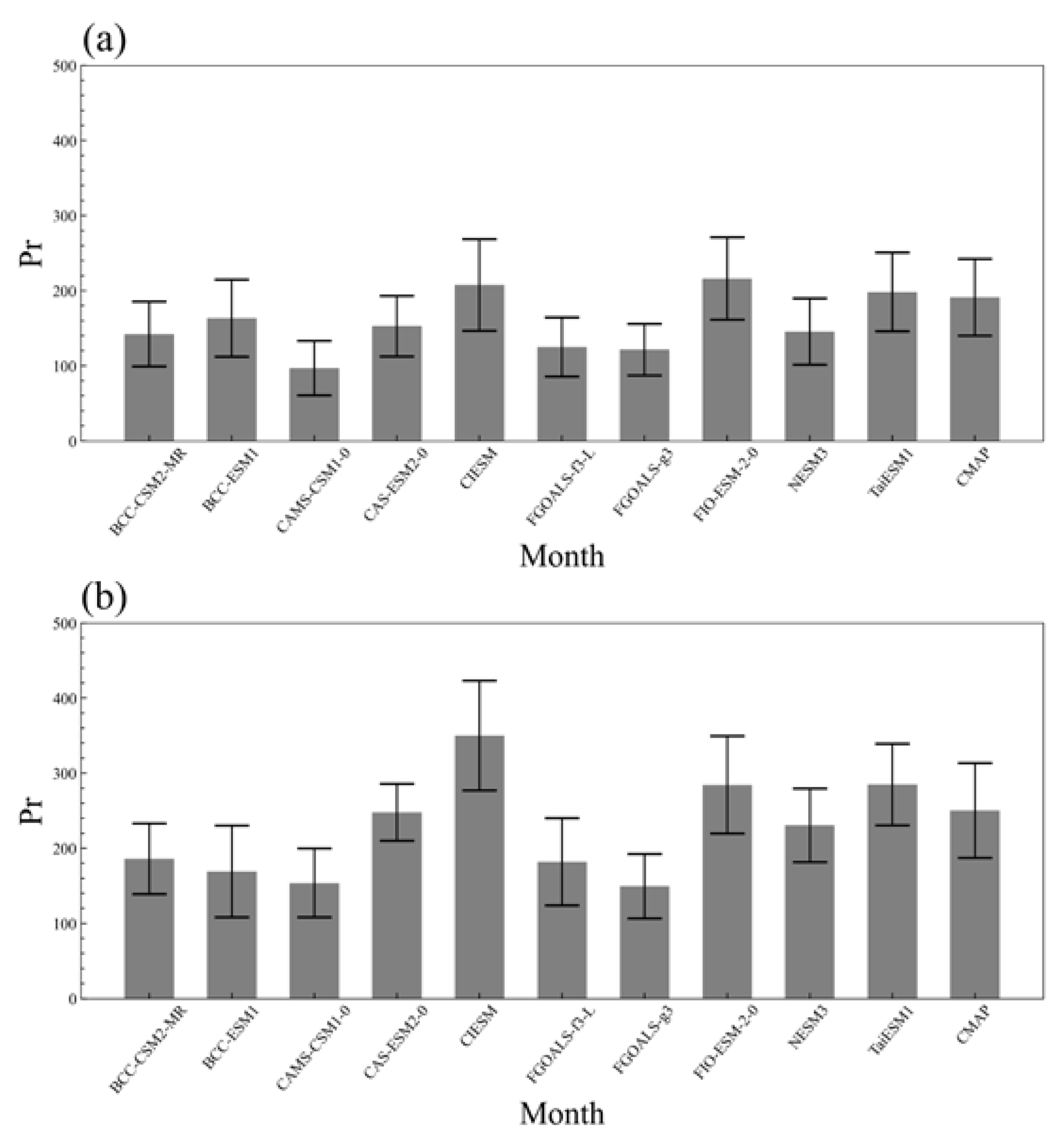
Figure 4 presents the climatology and variability of June rainfall in two focused regions, namely YHRV and SC. The monthly mean rainfall is ~190 mm in YHRV from the observations (Figure 4a). Seven models (Figure 3a–d,f,g,i) underestimate the average rainfall in the YHRV, while the remaining three models slightly overestimate the rainfall.
The average June precipitation in SC is ~250 mm from the observations. The underestimated seven models in SC are the same as that in YHRV. The remaining three models slightly overestimate the June rainfall. Therefore, the Chinese CMIP6 models have a systematic wet or dry bias across eastern China.

3.2. Physical Analysis of the SIC–China Rainfall Linkage

3.2.1. Relationship between the Kara–Barents SIC and June Precipitation in Eastern China

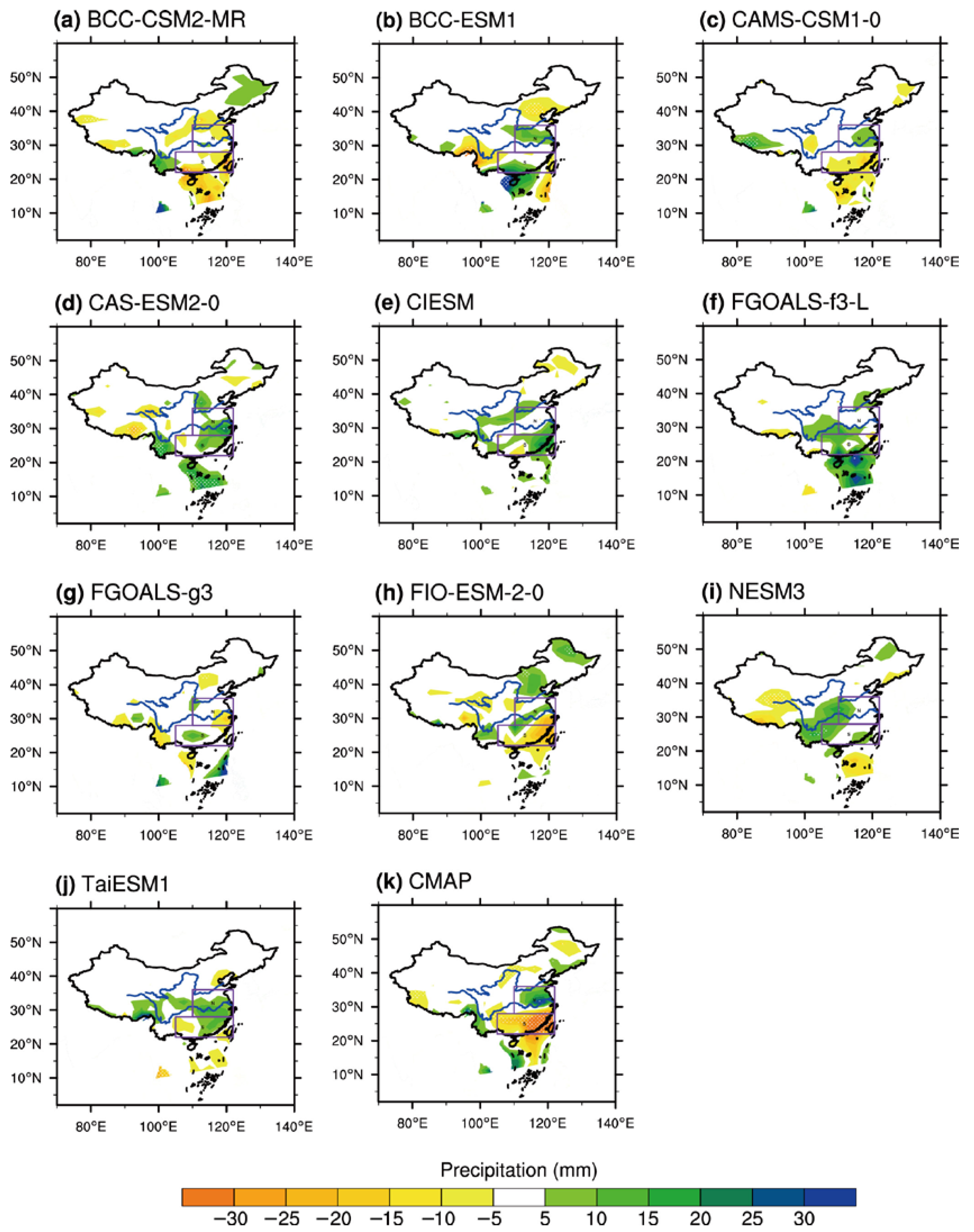
Several studies have explored how anomalous sea ice may influence atmospheric circulation and summer rainfall [13,27,29,31,53]. Yang et al. [25] found a potential lagged link between the Kara–Barents sea ice forcing and June precipitation in China. Figure 5 shows the regressed June rainfall against the SIC index in the Kara–Barents Sea in the preceding winter for the observations and 10 Chinese CMIP6 models. An observed dipole rainfall pattern forms in June across East China, and two strong response centers can be seen: one across YHRV (110–122°E, 28–36°N) and the other across SC (105–122°E, 22–28°N) (Figure 5k). Namely, a growth (loss) of Kara–Barents SIC in November and December corresponds to more (less) June precipitation in the north and less (more) precipitation in the south. However, very few models can simulate the observed sea ice–rainfall relationship (Figure 5a–j). This dipole rainfall pattern, namely dry in the south and wet in the north, is just roughly reproduced by two models (Figure 5c,h), although the amplitude is insignificant and weak. FGOALS-g3 simulates an overall opposite pattern to the observations (Figure 5g). However, a monopole or shifted rainfall patterns appear in other models in eastern China. BCC-CSM2-MR (Figure 5a) simulates a dry pattern across eastern China with the increase of sea ice, while the remaining models simulate a uniform wet pattern (Figure 5d–f,j). A wet pattern is reasonably captured in the north, but the signals are missing in the south in BCC-ESM1 (Figure 5b). NESM3 simulates a westward-shifted wet rainfall anomaly pattern. The simulated rainfall response to the Kara–Barents SIC diverges among the CMIP6 models, and it is common for the ten Chinese CMIP6 models to underrepresent the sea ice–rainfall relationship.

3.2.2. The Persistency of Ice

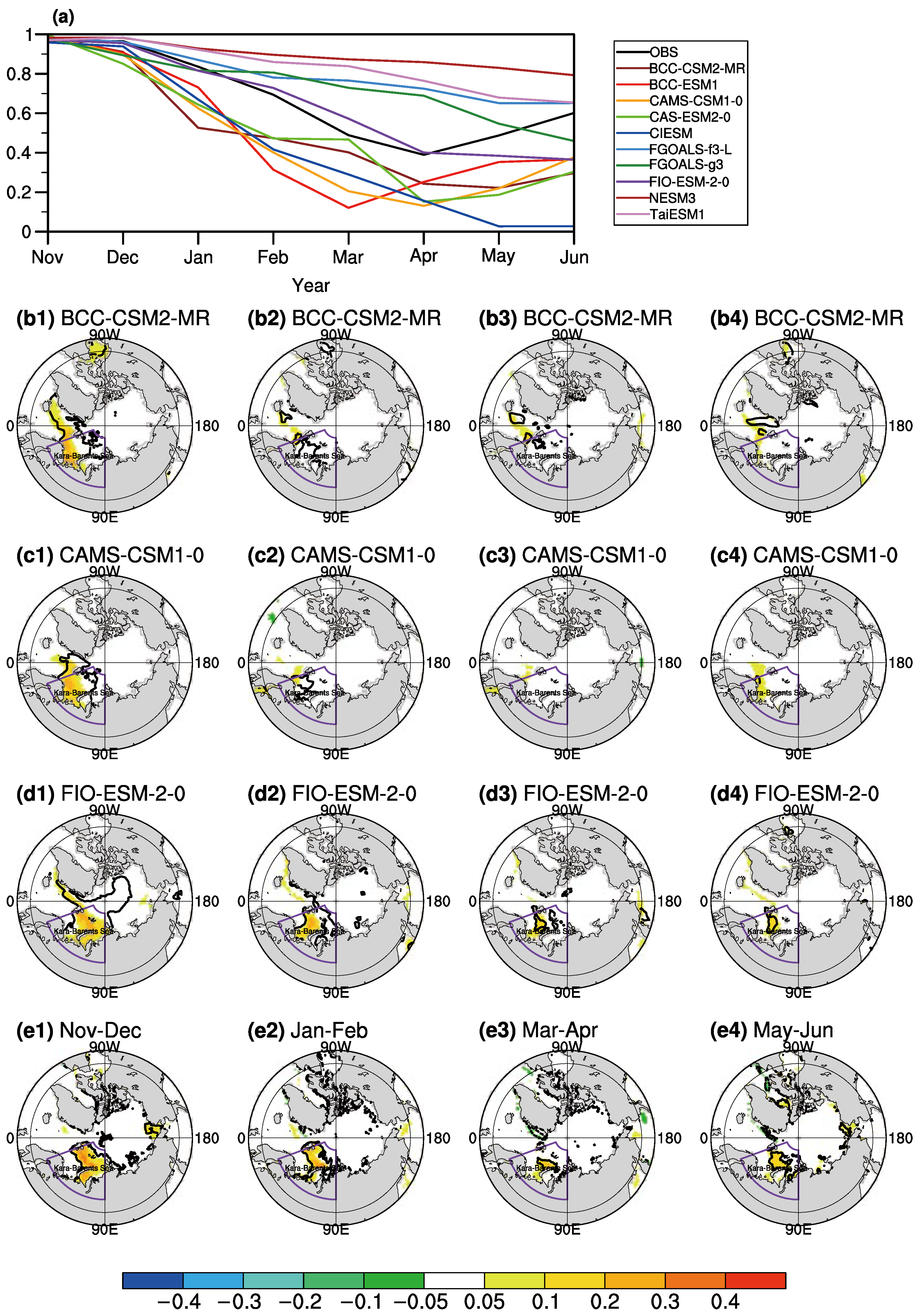
The connection between winter SIC in the Kara–Barents Seas and summer rainfall has been established in the reanalysis. However, it is still unclear how this pathway forms. The possible lagged impact of SIC is due to its long memory [25]. The evolution of the regressed standardized bimonthly Arctic SIC in the Kara–Barents Seas (20–90°E, 65–85°N) from early winter to early summer against the bimonthly (November–December mean) SIC index is shown in Figure 6 for the observations and 10 Chinese CMIP6 models.
In general, both the observations and models show a persistent weakening of SIC anomalies from November to June. From November to January, the Kara–Barents SIC anomalies weaken gradually but still do not diverge among the CMIP6 models. The self-persistency of SIC in two models (NESM3 and TaiESM1) is too strong, while it is too low in six models (Figure 1a–e,g). The overestimated (underestimated) SIC represents a longer (shorter) memory of SIC in models, which might lead to an underrepresentation of the SIC teleconnection. The seasonal evolution of the Kara–Barents SIC in FGOALS-f3-L and FIO-ESM-2-0 is similar to the observations.
The spatial distribution of SIC is largely biased from observations for nearly all models. The SIC variability is relatively independent in the Kara–Barents Seas in observations, while models simulate a relatively large covariance between Kara–Barents SIC and other Arctic regions (Figure 6b–e). The Kara–Barents SIC anomalies are significant in November–December and persist in January–February in observations. The area and coverage of SIC anomalies show significant shrinkage in March–April but still remain until May–June (Figure 6e). Three typical models are selected to examine the persistency of SIC in the Kara–Barents Seas, which respectively represent the too-strong, too-weak, and more realistic SIC memory in the Kara–Barents Seas as compared with observations. All three models simulate a larger SIC variability in the Arctic Ocean. Namely, the SIC variability is much larger in the models than in observations outside the Kara–Barents Seas. Therefore, the SIC variability in the Kara–Barents Seas from the CMIP6 models shows a larger dependence on that in other Arctic regions.

3.3. A Perspective from the Stratosphere–Troposphere Coupling

3.3.1. Stratospheric Circulation Anomalies following SIC Forcing

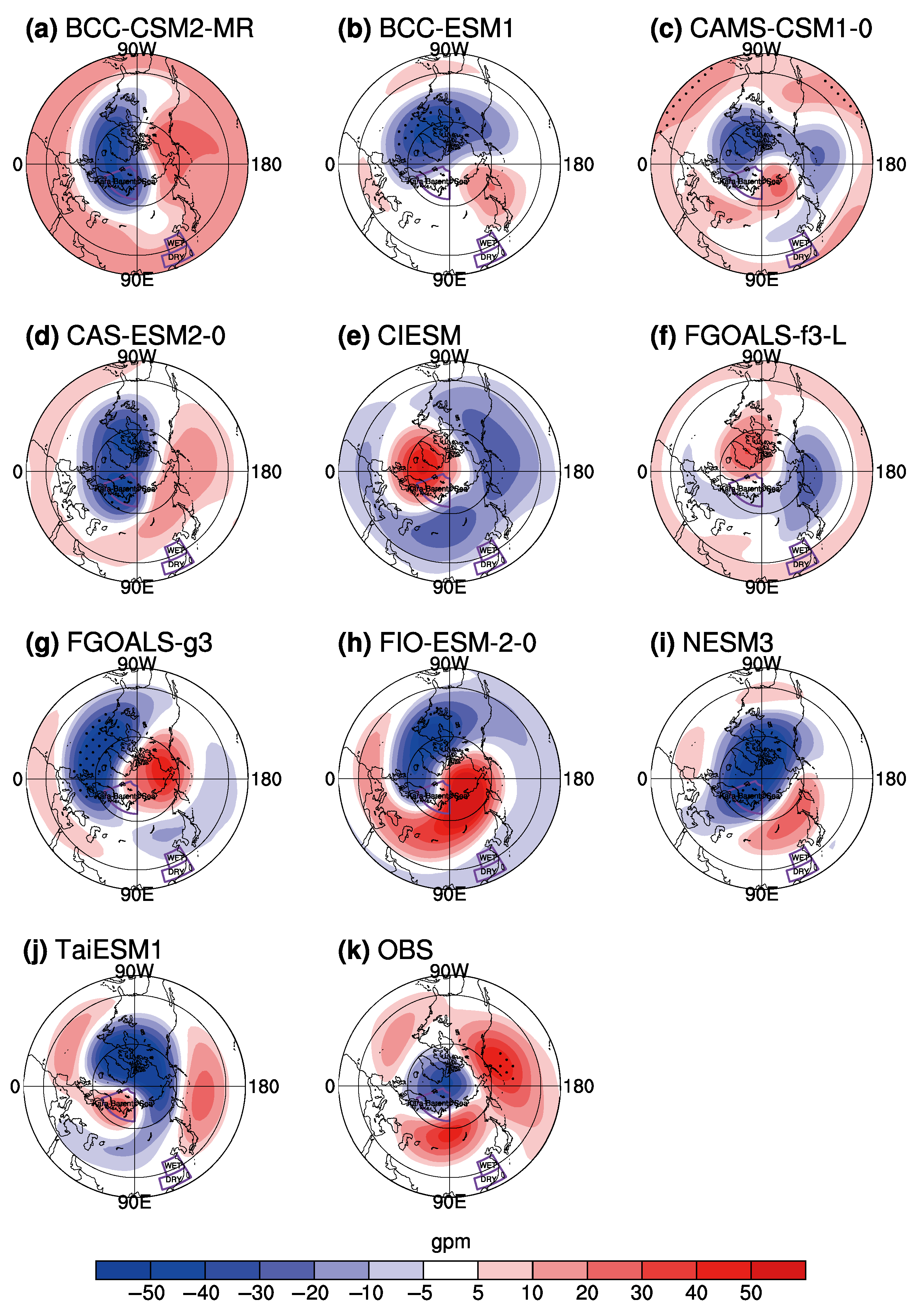
Figure 7 illustrates the concurrent regression of stratospheric circulation anomalies in November–December at 10 hPa against the Kara–Barents SIC index in November–December for both the CMIP6 models and the reanalysis. Significant height anomalies instantly occur in the stratosphere following the variability of Kara–Barents SIC in November–December (Figure 7k). The anomalous height structure exhibits a positive annular mode pattern in the Northern Hemisphere (NAM), corresponding to the strengthening of the stratospheric polar vortex. Previous studies have also identified a similar response in the stratosphere to the SIC decline over the Arctic [23,24,54]. Most of the Chinese CMIP6 models simulate a positive phase of the NAM in January–December. Specifically, most models reproduce a negative height anomaly patch over the Arctic. However, the NAM-like response is reversed in CIESM (Figure 7e). The positive NAM-like response is present in six models (Figure 7a–d,i,j). Three models (Figure 7f–h) simulate a strong wave-like response: the anomalous high and low distribute evenly in the circumpolar region. Those biases in the stratospheric anomalies associated with Kara–Barents SIC variability are possibly related to the biased in the mean state of the Arctic SIC and the too-strong covariance of the SIC variability.
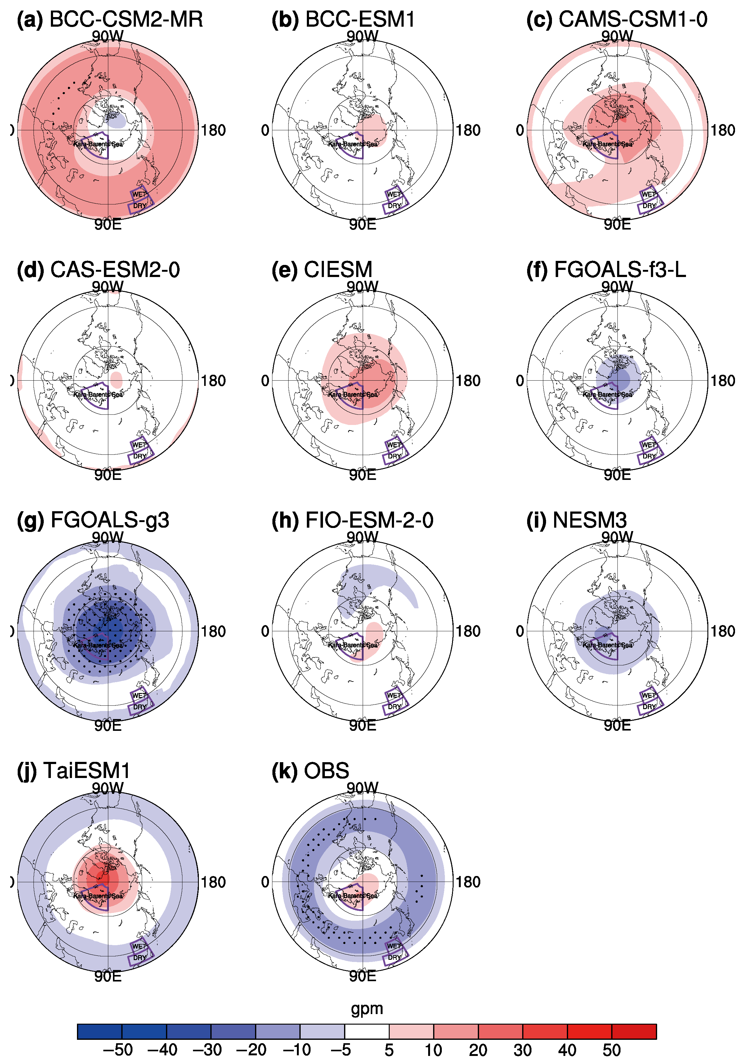
Yang et al. [25] indicated that the NAM response in the stratosphere is reversed in spring, which is possibly due to the fact that the suppressed waves in winter tend to break out in the following months and contribute to a weaker polar vortex. Hu et al. [26] also revealed this reversal of the stratospheric circulation anomalies from early winter to spring. The lead/lag regression of the bimonthly mean geopotential heights at 10 hPa in May–June against the Kara–Barents SIC index in November–December is illustrated in Figure 8 for the CMIP6 models and the reanalysis. Contrary to the stratospheric response in November and December, negative height anomalies are simulated in midlatitudes in May–June, while weak positive height anomalies can be seen in the Arctic stratosphere, most of which can be described by the negative phase of the NAM in the reanalysis (Figure 8k). The proficiency of the CMIP6 models is divergent in reproducing the negative NAM response. Nearly half of the models (Figure 8b,c,e,h,j) can reproduce the anomalous high in the Arctic stratosphere, with the most skillful one being TaiESM1 (Figure 8j). However, four models (Figure 8a,f,g,i) simulate a reversed height anomaly pattern. One model (Figure 8d) shows little anomalous height change.

3.3.2. Tropospheric Circulation Anomalies following SIC Forcing

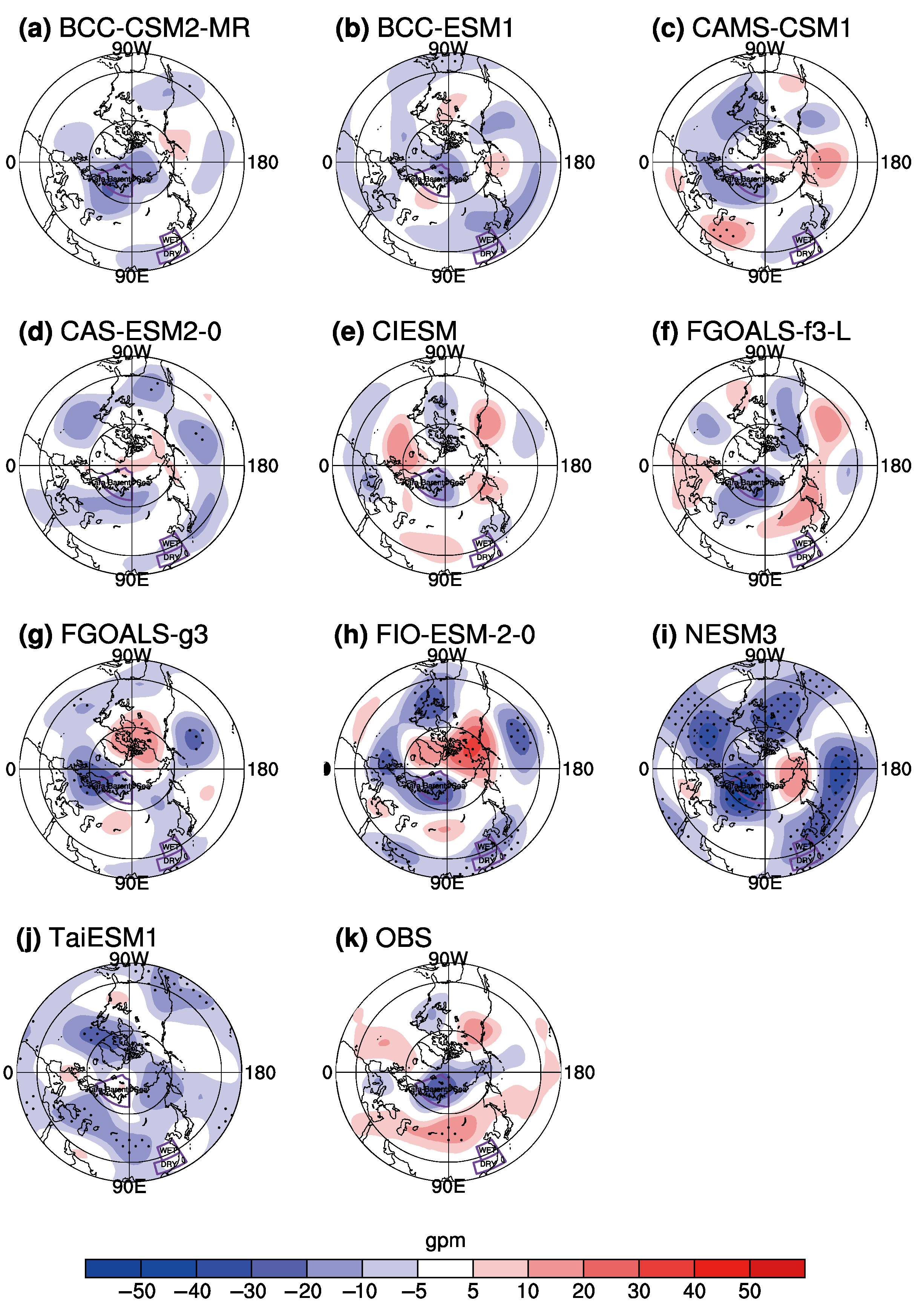
Figure 9 shows the regressed atmospheric circulation in November–December at 200 hPa against the Kara–Barents SIC index in November–December for both the CMIP6 models and the reanalysis. Similar to the stratospheric pattern, the midlatitudes are covered with anomalous highs, and the Arctic Ocean is covered with anomalous lows in the reanalysis from November to December (Figure 9k). The observed tropospheric height anomaly pattern also highly resembles the positive NAM pattern, although the high band in the midlatitudes is split, possibly due to the interference of the direct tropospheric response to SIC forcing. Namely, the Kara–Barents Seas is the region where the maximum negative height anomalies are observed. The negative height anomalies over the Kara–Barents Seas are simulated with different degrees of success (Figure 9a–j). The low response to the SIC forcing is biased from the Kara–Barents Seas in CAS-ESM2-0, which can be attributed to biases in the SIC variability. Three models (Figure 9a,i,j) simulate a too-homogenous low anomaly pattern. In contrast, the high responses are realistically present over northern Eurasia and around Greenland in four models (Figure 9b,e–g). Namely, the tropospheric response behaves in a wave train pattern emitting from the Kara–Barents Seas linked with the thermal forcing, although the NAM pattern is clearly observed from the stratosphere. Yang et al. [25] suggested that the tropospheric response in midwinter and spring is a combination of the stratospheric pathway and tropospheric wave train directly forced by SIC forcing.
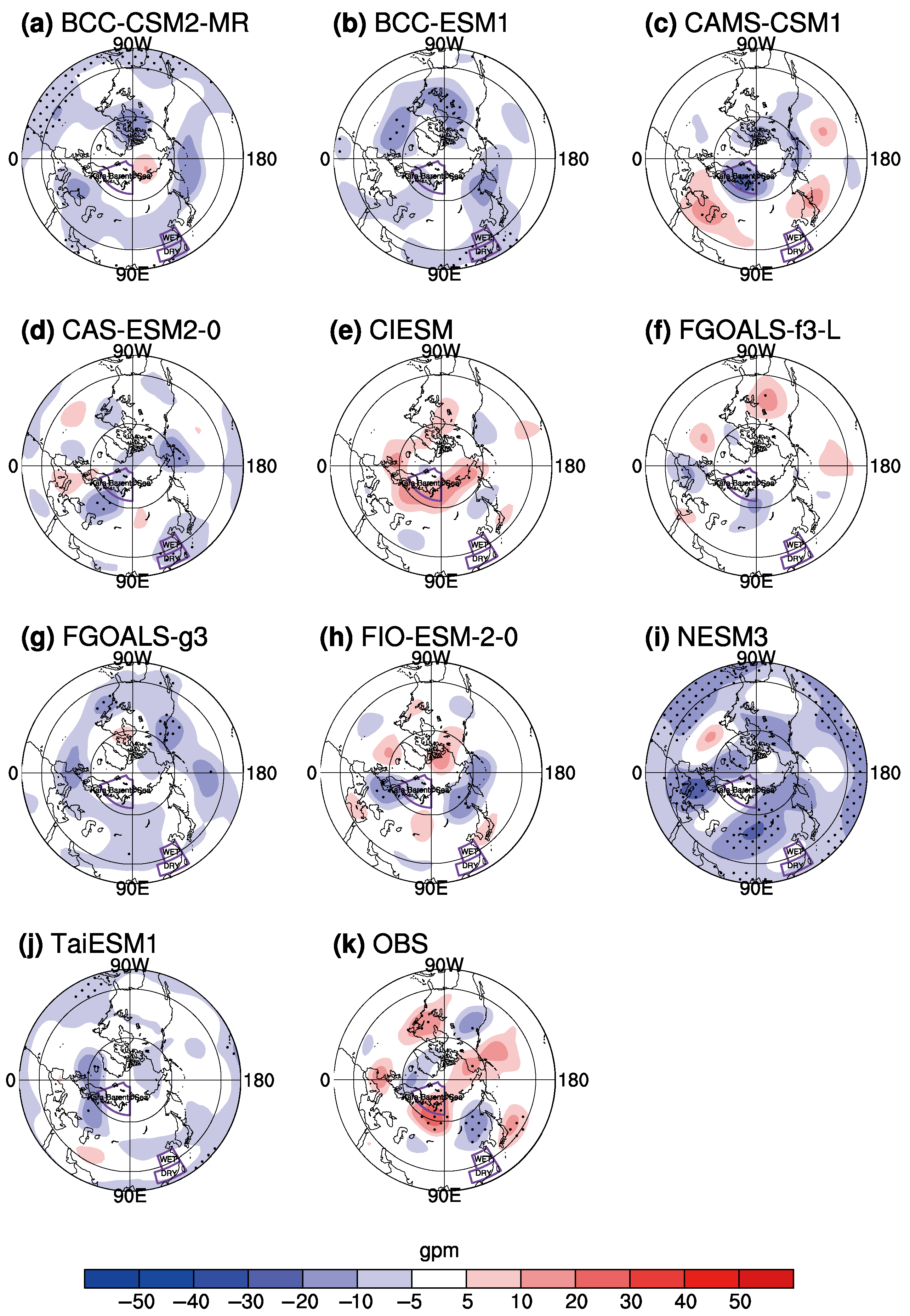
Tropospheric height anomalies in the summer following Kara–Barents SIC forcing are shown in Figure 10 for the CMIP6 models and observations. Different from the response in the winter, a positive local height anomaly lobe forms in May and June following a SIC growth in the Kara–Barents Seas (Figure 10k). A negative lobe can be seen over northeast Asia, while a positive lobe forms in the adjacent ocean near Japan. However, most models cannot simulate the wave train across the Kara–Barents Seas, Asia, and the Pacific. Specifically, illusive anomalous lows from the Kara–Barents Seas to East Asia and the northeast Pacific are simulated by six models (Figure 10a,b,d,f,g,i,j). All CMIP6 models simulate a less organized wave train response than seen in the observations. The overestimated covariance between the SIC in most regions of the Arctic mask the pure impact of the SIC forcing from the Kara–Barents Seas. Very few models except FIO-ESM-2-0 can simulate the low response in northeast Asia and the high response in Japan.
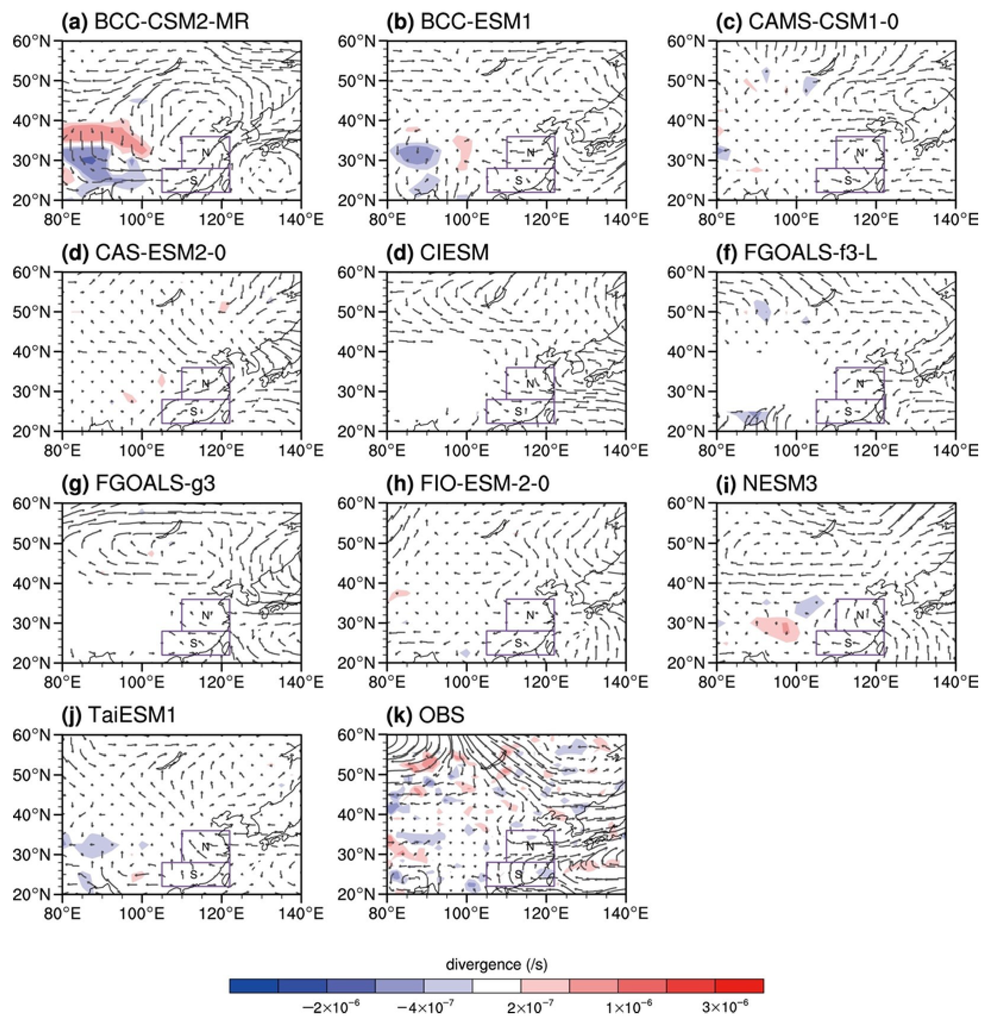
Figure 11 presents the lead/lag regression of circulation anomalies at 700 hPa during May–June against the Kara–Barents SIC index in early winter. In consistence with the height anomaly lobes at 200 hPa, an anticyclone forms over the northeastern Pacific Ocean, and an anomalous cyclone appears in northeast China, respectively. The northerly anomalies appear in eastern China, west of the cyclone, and converge with the southwesterly anomalies in YHRV (Figure 11k), which successfully explain the local wet conditions in June. Most models fail to simulate the anomalous anticyclone over the northwest Pacific and the cyclone over northeast China (Figure 11a–g). BCC-CSM2-MR simulates an anomalous anticyclone over the sea and an anomalous cyclone in northern China. Southerly anomalies also appear over the eastern coasts of China and converge with the northwesterly anomalies in YHRV. Although the circulation centers are not evident in CAS-ESM2-0, the southwesterly anomalies from SC to YHRV are reproduced. Three models (FGOALS-g3, NESM3, and TaiESM1) simulate the southeasterly anomalies over eastern China, which bring abundant moist air. Two models (BCC-ESM1 and CAMS-CSM1-0) simulate anomalous northeasterlies in the north and anomalous southwesterlies in the south, corresponding to the local increased precipitation for those two models. The convergence between southeasterlies and northeasterlies in SC is modeled by CIESM, corresponding to the local wet conditions.

3.3.3. Possible Delay via the Troposphere–Stratosphere Coupling

The potential sea ice–rainfall relationship can also be explained in view of cryosphere–troposphere–stratosphere coupling. Troposphere–stratosphere interactions are strongly related to the stratospheric polar vortex [24]. Figure 12 illustrates the regressed circumpolar wind against the Kara–Barents SIC index in early winter. The polar vortex in the stratosphere instantly strengthens from November to February when the Kara–Barents SIC increases (Figure 12k). The strengthened polar vortex is followed by its weakening in the spring. The anomalies in the stratosphere and the sign reversal from anomalous westerlies to easterlies show a gradual downward propagation. In winter, the downward-propagating signal can reach the near-surface, while it can only reach the upper troposphere in spring and early summer. Most models largely underestimate the intensifying response of the vortex (Figure 12a–j). The high-level response to the SIC forcing is missing in CAMS-CSM1-0, and the strengthening response of the vortex is too fast and short in BCC-CSM2-MR and NESM3.
Only two models (BCC-ESM1 and CIESM) can simulate the positive zonal wind anomalies in the winter, but the wind reversal is missing. Anomalous easterlies are observed before May and June throughout the stratosphere and troposphere. Three models (BCC-CSM2-MR, NESM3, and TaiESM1) simulate the easterly anomalies before May and June, although the seasonal evolution of the wind anomalies shows slight biases from observations. In short, the observed stratosphere–troposphere–cryosphere coupling is not simulated in most CMIP6 models, which further limits the reproducibility of the linkage between the SIC forcing and rainfall in China. It is still a challenge for the modeling groups to improve the SIC simulation, especially for the air–SIC interaction over the Arctic.

4. Conclusions

The possible effect of SIC forcing in the Kara–Barents Seas on summer rainfall in China has been observed in previous studies. However, the general performance of the CMIP6 models in reproducing the SIC–rainfall relationship has not previously been examined. A better understanding of the SIC–rainfall relation and its simulation in models is necessary for model development. The main findings of this article are as follows.
The long-term climatology and variability of Arctic SIC are compared for ten Chinese CMIP6 models. The full SIC is located in most of the Arctic Ocean, where the SIC variability is very small in winter. The largest SIC variability is mainly situated along the edge of the Arctic SIC and the transition between the Arctic Ocean and continents—open sea water. A typical region is the Kara–Barents Seas, where the observed SIC variability is evident and relatively independent from that in other Arctic regions. Most models reasonably simulate the overall SIC distribution, and six models slightly overestimate the SIC in the transition zone. However, models tend to simulate too large a SIC covariance between the Kara–Barents Seas and other Arctic regions.
The long-term mean and variability of June precipitation in eastern China are also examined for CMIP6 models as compared to CMAP. All models simulate the general distribution of rainfall climatology and variability: both the variability and the climatology of rainfall in China decrease from the southeast to the northwest. However, the rainfall variability in most models is larger than in observations.
The relationship between Arctic SIC in winter and rainfall in summer over East China is also investigated for models. In observations, the Kara–Barents sea ice anomaly is linked to the dipole rainfall structure in eastern China afterward. When sea ice increases, the YHRV becomes wetter, and the SC becomes drier, respectively. This dipole rainfall pattern is simulated with varying success. The dipole rainfall structure can only be simulated by two models, although they underestimate the central amplitude of rainfall anomalies connected to SIC forcing. The remaining models simply simulate a monopole or a shifted rainfall pattern as compared with observations.
Possible factors for the missing SIC–rainfall relationship in the models include the biases in the long memory of the Arctic SIC, underrepresentation of the circulation related to the SIC anomalies, and misrepresentation of the stratosphere–troposphere coupling. In observations, the Kara–Barents sea ice anomaly remains from November to June, while the models behave with a widespread persistency of the SIC anomalies. Further, the observed variability of Kara–Barents SIC is relatively independent of that in other Arctic regions, while the SIC variability in the Kara–Barents Seas simulated by models covary with that in other Arctic regions, which dampens the mere influence of the Kara–Barents SIC forcing.
The atmospheric circulation anomalies forced by the Kara–Barents SIC variation change with the season. An annular mode pattern instantly forms in winter, which is reversed in the stratosphere in spring. In early summer, the annular mode response in the troposphere is entangled with a wave train excited across the Kara–Barents Seas, Asia, and the Pacific. Due to the convergence of anomalous southwesterly and northeasterly winds over YHRV, a dipole pattern (wet YHRV–dry SC) is eventually generated in June. In early winter, the positive NAM response is simulated in most models, while the negative NAM is not easy to reproduce in spring for most models. The models are also unable to simulate the reversal of the stratospheric NAM response, and the tropospheric wave-like pattern is also shifted or missing in the models.
Most Chinese models produce the general distribution of the concurrent stratospheric circulation anomalies related to the SIC anomalies in early winter. However, CMIP6 models still do not well resolve the lagged impact of SIC on midlatitude circulation and rainfall in China. The reproducibility of the SIC variability in the Kara–Barents seas is still low at present, and the overestimated coherence of the Arctic SIC is commonly present in models. Further, biases in the stratospheric response to SIC further increase uncertainties in the response of tropospheric circulation from winter to summer via stratosphere–troposphere coupling. Considering biases in the stratosphere, rainfall, and sea ice are still widely present in the models, it is still a challenge for Chinese modeling groups to further improve the stratosphere–troposphere–cryosphere coupling simulation.

Author Contributions

Formal analysis, H.Y., H.C. and Q.L.; funding acquisition, J.R.; investigation, H.Y. and J.R.; software, H.Y. and J.R.; supervision, J.R. and J.L.; validation, H.Y., J.R. and H.C.; visualization, H.Y. and J.R.; writing—original draft preparation, H.Y. and J.R. All authors have read and agreed to the published version of the manuscript.

Funding

This research was funded by the National Natural Science Foundation of China (grant nos. 42030605 and 42175069) and the College Students’ Practice Innovation Training Program of Jiangsu Province, NUIST Students’ Platform for Innovation and Entrepreneurship Training Program (Project 202210300004Z).

Data Availability Statement

The SIC data were provided by the UK Met Office at https://www.metoffice.gov.uk (accessed on 1 April 2022). The CMAP precipitation data can be downloaded at https://psl.noaa.gov/ (accessed on 1 April 2022). The ERA5 reanalysis is available at https://www.ecmwf.int (accessed on 1 April 2022).

Acknowledgments

The authors thank the ESGF, UKMO, and ECMWF for their free datasets.

Conflicts of Interest

The authors declare no conflict of interest.

References

  1. Curry, J.A.; Schramm, J.L.; Ebert, E.E. Sea ice-albedo climate feedback mechanism. J. Clim. 1995, 8, 240–247. [Google Scholar] [CrossRef]
  2. Lukovich, J.V.; Barber, D.G. Atmospheric controls on sea ice motion in the southern Beaufort Sea. J. Geophys. Res. 2006, 111, D18103. [Google Scholar] [CrossRef]
  3. Balmaseda, M.A.; Ferranti, L.; Molteni, F.; Palmer, T.N. Impact of 2007 and 2008 Arctic ice anomalies on the atmospheric circulation: Implications for long-range predictions. Meteorol. Soc. 2010, 136, 1655–1664. [Google Scholar] [CrossRef]
  4. Serreze, M.C.; Holland, M.M.; Stroeve, J. Perspectives on the Arctic’s shrinking sea-ice cover. Science 2007, 315, 1533–1536. [Google Scholar] [CrossRef] [PubMed]
  5. Li, F.; Wang, H.J.; Gao, Y.Q. On the strengthened relationship between East Asian winter monsoon and Arctic Oscillation: A comparison of 1950–1970 and 1983–2012. J. Clim. 2014, 27, 5075–5091. [Google Scholar] [CrossRef]
  6. Gimeno, L.; Vázquez, M.; Eiras-Barca, J.; Sorí, R.; Algarra, I.; Nieto, R. Atmospheric moisture transport and the decline in Arctic Sea ice. Wires. Clim. Chang. 2019, 10, e588. [Google Scholar] [CrossRef]
  7. Tang, Q.; Zhang, X.; Francis, J.A. Extreme summer weather in northern mid-latitudes linked to a vanishing cryosphere. Nat. Clim. Chang. 2014, 4, 45–50. [Google Scholar] [CrossRef]
  8. Rao, J.; Garfinkel, C.I.; Wu, T.; Luo, J.; Lu, Y.; Chu, M.; Lu, Q. Combined modes of the northern stratosphere, tropical oceans, and East Asian spring rainfall: A novel method to improve seasonal forecasts of precipitation. Geophys. Res. Lett. 2023, 50, e2022GL101360. [Google Scholar] [CrossRef]
  9. Liu, J.P.; Curry, J.A.; Wang, H.; Song, M.; Horton, R. Impact of declining Arctic sea ice on winter snowfall. Proc. Natl. Acad. Sci. USA 2012, 109, 4074–4079. [Google Scholar] [CrossRef]
  10. Gao, T.; Yu, J.Y.; Paek, H. Impacts of four northernhemisphere teleconnection patterns on atmospheric circulations over Eurasia and the Pacific. Theor. Appl. Climatol. 2017, 129, 815–831. [Google Scholar] [CrossRef]
  11. Francis, J.; Vavrus, S. Evidence linking Arctic amplification to extreme weather in mid-latitudes. Geophys. Res. Lett. 2012, 39, L06801. [Google Scholar] [CrossRef]
  12. Outten, S.D.; Esau, I. A link between Arctic sea ice and recent cooling trends over Eurasia. Clim. Chang. 2012, 110, 1069–1075. [Google Scholar] [CrossRef]
  13. Wu, B.Y.; Zhang, R.H.; D’Arrigo, R.; Su, J. On the relationship between winter sea ice and summer atmospheric circulation over Eurasia. J. Clim. 2013, 26, 5523–5536. [Google Scholar] [CrossRef]
  14. Ji, L.; Fan, K. Interannual linkage between wintertime sea-ice cover variability over the Barents Sea and springtime vegetation over Eurasia. Clim. Dyn. 2019, 53, 5637–5652. [Google Scholar] [CrossRef]
  15. Honda, M.; Inoue, J.; Yamane, S. Influence of low Arctic sea ice minima on anomalously cold Eurasian winters. Geophys. Res. Lett. 2009, 36, L08707. [Google Scholar] [CrossRef]
  16. Petoukhov, V.; Semenov, V.A. A link between reduced Kara-Barents sea ice and cold winter extremes over northern continents. J. Geophys. Res. 2010, 115, D21. [Google Scholar] [CrossRef]
  17. Wu, B.; Su, J.; Zhang, R. Effects of autumn–winter Arctic sea ice on winter Siberian High. Chin. Sci. Bull. 2011, 56, 3220–3228. [Google Scholar] [CrossRef]
  18. Mori, M.; Watanabe, M.; Shiogama, H.; Inoue, J.; Kimoto, M. Robust Arctic sea-ice influence on the frequent Eurasian cold winters in past decades. Nat. Geosci. 2014, 7, 869–873. [Google Scholar] [CrossRef]
  19. Jang, Y.; Jun, S.; Son, S.; Min, S.; Kug, J. Delayed Impacts of Arctic Sea-Ice Loss on Eurasian Severe Cold Winters. J. Geophys. Res. Atmos. 2021, 126, e2021JD035286. [Google Scholar] [CrossRef]
  20. He, Y.; Zhu, X.; Sheng, Z.; He, M.; Feng, Y. Observations of Inertia Gravity Waves in the Western Pacific and Their Characteristic in the 2015/2016 Quasi-biennial Oscillation Disruption. J. Geophys. Res. Atmos. 2020, 127, e2022JD037208. [Google Scholar] [CrossRef]
  21. Ji, Q.; Zhu, X.; Sheng, Z.; Tian, T. Spectral Analysis of Gravity Waves in the Martian Thermosphere during Low Solar Activity Based on MAVEN/NGIMS Observations. Astrophys. J. 2022, 938, 97. [Google Scholar] [CrossRef]
  22. Zhang, J.; Ji, Q.; Sheng, Z.; He, M.; He, Y.; Zuo, X.; He, Z.; Qin, Z.; Wu, G. Observation based climatology Martian atmospheric waves perturbation Datasets. Sci. Data 2023, 10, 4. [Google Scholar] [CrossRef] [PubMed]
  23. Kim, B.M.; Son, S.W.; Min, S.K.; Jeong, J.H.; Kim, S.J.; Zhang, X.; Shim, T.; Yoon, J.H. Weakening of the stratospheric polar vortex by Arctic sea-ice loss. Nat. Commun. 2014, 5, 4646. [Google Scholar] [CrossRef] [PubMed]
  24. Cohen, J.; Agel, L.; Barlow, M.; Garfinkel, C.I.; White, I. Linking Arctic variability and change with extreme winter weather in the United States. Science 2021, 373, 1116–1121. [Google Scholar] [CrossRef] [PubMed]
  25. Yang, H.; Rao, J.; Chen, H. Possible lagged impact of the Arctic sea ice in Barents–Kara Seas on June precipitation in Eastern China. Front. Earth Sci. 2022, 10, 886192. [Google Scholar] [CrossRef]
  26. Hu, J.; Ren, R.; Xu, H. Occurrence of winter stratospheric sudden warming events and the seasonal timing of spring stratospheric final warming. J. Atoms. Sci. 2014, 71, 2319–2334. [Google Scholar] [CrossRef]
  27. Screen, J.A. Influence of Arctic sea ice on European summer precipitation. Environ. Res. Lett. 2013, 8, 044015. [Google Scholar] [CrossRef]
  28. Wang, H.; He, S. The North China/Northeastern Asia severe summer drought in 2014. J. Clim. 2015, 28, 6667–6681. [Google Scholar] [CrossRef]
  29. Wu, B.Y.; Zhang, R.H.; Wang, B. On the association between a spring Arctic sea ice concentration and Chinese summer rainfall: A further study. Adv. Atmos. Sci. 2009, 26, 666–678. [Google Scholar] [CrossRef]
  30. Liu, Y.; Chen, H.P.; Wang, H.J.; Sun, J.Q.; Li, H.; Qiu, Y.B. Modulation of the Kara Sea ice variation on the ice freeze-up time in Lake Qinghai. J. Clim. 2019, 32, 2553–2568. [Google Scholar] [CrossRef]
  31. Zhao, P.; Zhang, X.; Zhou, X.; Ikeda, M.; Yin, Y. The sea ice extent anomaly in the north pacific and its impact on the East Asian summer monsoon rainfall. J. Clim. 2004, 17, 3434–3447. [Google Scholar] [CrossRef]
  32. Han, T.; Chen, H.; Wang, H. Recent changes in summer precipitation in Northeast China and the background circulation. Int. J. Climatol. 2015, 35, 4210–4219. [Google Scholar] [CrossRef]
  33. He, S.P.; Gao, Y.Q.; Furevik, T.; Wang, H.J.; Li, F. Teleconnection between sea ice in the Barents Sea in June and the Silk Road, Pacific-Japan and East Asian rainfall patterns in August. Adv. Atmos. Sci. 2018, 8, 376–382. [Google Scholar] [CrossRef]
  34. Li, F.; Wang, H.J.; Gao, Y.Q. Change in sea ice cover is responsible for non-uniform variation in winter temperature over East Asia. Atmos. Ocean. Sci. Lett. 2015, 8, 376–382. [Google Scholar]
  35. Wang, H.J.; Chen, H.P.; Liu, J.P. Arctic sea ice decline intensified haze pollution in eastern China. Atmos. Ocean. Sci. Lett. 2015, 8, 120–122. [Google Scholar]
  36. Zhang, P.; Wu, Y.; Simpson, I.R.; Smith, K.L.; Zhang, X.; De, B.; Callaghan, P. A stratospheric pathway linking a colder Siberia to Barents-Kara Sea sea ice loss. Sci. Adv. 2018, 4, eaat6025. [Google Scholar] [CrossRef] [PubMed]
  37. Zhang, R.; Screen, J.A. Diverse Eurasian winter temperature responses to Barents-Kara sea ice anomalies of different magnitudes and seasonality. Geophys. Res. Lett. 2021, 48, e2021GL092726. [Google Scholar] [CrossRef]
  38. Zhang, R.; Sun, C.; Zhang, R.; Jia, L.; Li, W. The impact of Arctic sea ice on the inter annual variations of summer Ural blocking. Int. J. Climatol. 2018, 38, 4632–4650. [Google Scholar] [CrossRef]
  39. Wu, Z.; Li, J.; Jiang, Z.; He, J. Predictable climate dynamics of abnormal East Asian winter monsoon: Once-in-a-century snowstorms in 2007/2008 winter. Clim. Dyn. 2011, 37, 1661–1669. [Google Scholar] [CrossRef]
  40. Li, S.; Hou, W.; Feng, G. Atmospheric circulation patterns over East Asia and their connection with summer precipitation and surface air temperature in Eastern China during 1961–2013. J. Meteorol. Res. 2018, 2, 203–218. [Google Scholar] [CrossRef]
  41. Han, T.T.; He, S.P.; Wang, H.J.; Hao, X. Variation in principal modes of midsummer precipitation over Northeast China and its associated atmospheric circulation. Adv. Atmos. Sci. 2019, 36, 55–64. [Google Scholar] [CrossRef]
  42. Wang, J.; Guo, Y. Possible impacts of Barents Sea ice on the Eurasian atmospheric circulation and rainfall of East China in the beginning of summer. Adv. Atmos. Sci. 2004, 21, 662–674. [Google Scholar] [CrossRef]
  43. Zhang, G.; Zeng, G.; Yang, X.; Iyakaremye, V. Two spatial types of North China heatwaves and their possible links to Barents-Kara Sea ice changes. Int. J. Climatol. 2022, 24, 6876–6889. [Google Scholar] [CrossRef]
  44. Han, T.; Zhang, M.; Zhu, J.; Zhou, B.; Li, S. Impact of early spring sea ice in Barents Seas on midsummer rainfall distribution at Northeast China. Clim. Dyn. 2021, 57, 1023–1037. [Google Scholar] [CrossRef]
  45. Wu, T.; Lu, Y.; Fang, Y.; Xin, X.; Li, L.; Li, W.; Jie, W.; Liu, Y.; Zhang, L.; Zhang, F.; et al. The Beijing Climate Center Climate System Model (BCC-CSM): The main progress from CMIP5 to CMIP6. Geosci. Model Dev. 2019, 12, 1573–1600. [Google Scholar] [CrossRef]
  46. Wyser, K.; Nojie, T.V.; Yang, S.; Hardenberg, J.V.; O’Donnell, D.; Döscher, R. On the increased climate sensitivity in the EC-Earth model from CMIP5 to CMIP6. Geosci. Model Dev. 2019, 13, 3456–3474. [Google Scholar] [CrossRef]
  47. Watts, M.; Maslowski, W.; Lee, Y.J.; Kinney, J.C.; Osinski, R. A spatial evaluation of Arctic sea ice and regional limitations in CMIP6 historical simulations. J. Clim. 2021, 34, 6399–6420. [Google Scholar] [CrossRef]
  48. Rayner, N.A.; Parker, D.E.; Horton, E.B.; Folland, C.K.; Alexander, L.V.; Rowell, D.P.; Kent, E.C.; Kaplan, A. Global analyses of sea surface temperature, sea ice, and night marine air temperature since the late nineteenth century. J. Geophys. Res. Atmos. 2003, 108, 4407. [Google Scholar] [CrossRef]
  49. Hersbach, H.; Bell, B.; Berrisford, P.; Hirahara, S.; Horanyi, A.; Munoz-Sabater, J.; Nicolas, J.; Peubey, C.; Radu, R.; Schepers, D.; et al. The ERA5 global reanalysis. Q. J. R. Meteorol. Soc. 2020, 146, 1999–2049. [Google Scholar] [CrossRef]
  50. Xie, P.; Arkin, P.A. Global Precipitation: A 17-Year Monthly Analysis Based on Gauge Observations, Satellite Estimates, and Numerical Model Outputs. Bull. Am. Meteorol. Soc. 1997, 78, 2539–2558. [Google Scholar] [CrossRef]
  51. Long, M.; Zhang, L.; Hu, S.; Qian, S. Multi-aspect assessment of CMIP6 models for Arctic sea ice simulation. J. Clim. 2021, 34, 1515–1529. [Google Scholar] [CrossRef]
  52. Guo, D.; Gao, Y.; Bethke, I.; Gong, D.; Johannessen, O.M.; Wang, H.J. Mechanism on how the spring Arctic sea ice impacts the East Asian summer monsoon. Theor. Appl. Climatol. 2014, 115, 107–119. [Google Scholar] [CrossRef]
  53. Vihma, T. Effects of Arctic Sea Ice Decline on Weather and Climate: A Review. Surv. Geophys. 2014, 35, 1175–1214. [Google Scholar] [CrossRef]
  54. Hoshi, K.; Ukita, J.; Nakamura, T.; Yamazaki, K.; Miyoshi, Y.; Jaiser, R. Weak stratospheric polar vortex events modulated by the Arctic sea ice loss. J. Geophys. Res. Atmos. 2019, 124, 441–1193. [Google Scholar] [CrossRef]
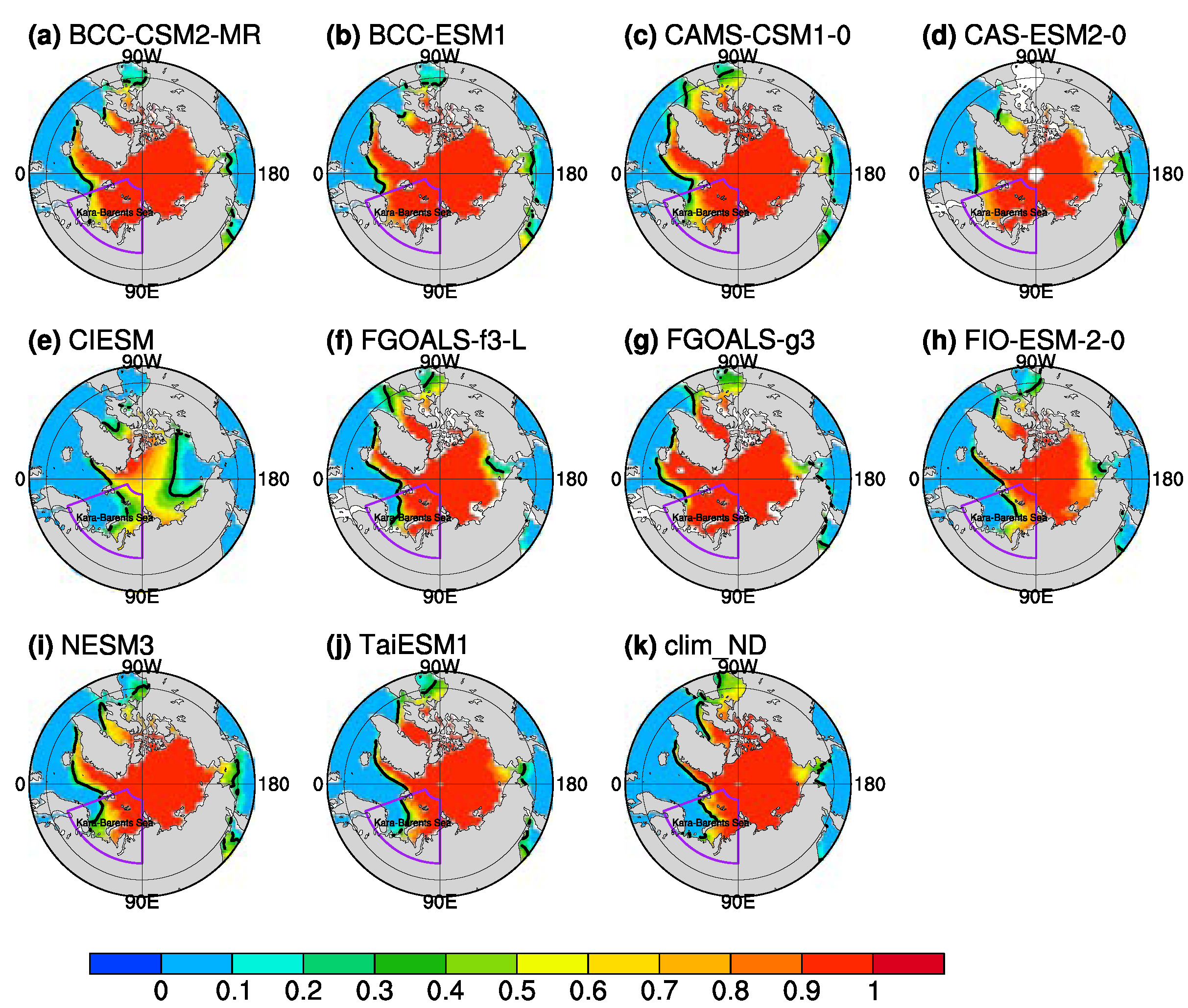
Figure 1. Climatology of the Northern Hemisphere SIC in November and December for (aj) ten CMIP6 models and (k) observations. The Kara–Barents Seas (20–90°E, 65–85°N) are marked in the box.
Remotesensing 15 02111 g001
Figure 2. As in Figure 1, but for the standard deviation of the Northern Hemisphere SIC in November and December for (aj) ten CMIP6 models and (k) observations.
Remotesensing 15 02111 g002
Figure 3. Climatology (contours; units: mm) and variability (shaded; units: mm) of June rainfall for (aj) ten CMIP6 models and (k) CMAP observations. The relatively large rainfall variability centers are shown in purple boxes, i.e., the YHRV (110–122°E, 28–36°N) and SC (105–122°E, 22–28°N).
Remotesensing 15 02111 g003
Figure 4. The mean state (gray bars) and standard deviation (error bars) of the June precipitation (units: mm) in (a) the YHRV and (b) SC for CMIP6 models and CMAP observations.
Remotesensing 15 02111 g004
Figure 5. Lagged regression of June rainfall (units: mm) against the standardized Kara–Barents SIC index in November–December for (aj) ten CMIP6 models and (k) CMAP observations. The purple boxes mark the YHRV (110–122°E, 28–36°N) and SC (105–122°E, 22–28°N) regions. Regressions are highlighted with dots if they are above the 95% confidence level.
Remotesensing 15 02111 g005
Figure 6. (a) Regressed bimonthly Arctic SIC anomalies against the Kara–Barents SIC index in November–December for ten CMIP6 models and observations as a representation of the SIC persistency. (be) Spatiotemporal evolution of regressed SIC anomalies from early winter to early summer against the standardized Kara–Barents SIC index for three typical CMIP6 models and observations. The regression is marked by black contours if it is above the 95% confidence level.
Remotesensing 15 02111 g006
Figure 7. Concurrent regression of bimonthly mean heights at 10 hPa (units: gpm) in November–December against the standardized Kara–Barents SIC index for (aj) ten CMIP6 models and (k) observations. Regressions are highlighted with dots if they are above the 95% confidence level.
Remotesensing 15 02111 g007
Figure 8. Lead/lag regression of bimonthly mean geopotential heights at 10 hPa (units: gpm) in May–June against the standardized Kara–Barents SIC index in early winter for (aj) ten CMIP6 models and (k) observations. Regressions are highlighted with dots if they are above the 95% confidence level.
Remotesensing 15 02111 g008
Figure 9. Concurrent regression of bimonthly mean heights at 200 hPa (units: gpm) in November–December against the standardized Kara–Barents SIC index for (aj) ten CMIP6 models and (k) observations. Regressions are highlighted with dots if they are above the 95% confidence level.
Remotesensing 15 02111 g009
Figure 10. Lead/lag regression of bimonthly mean geopotential heights at 200 hPa (units: gpm) in May–June against the standardized Kara–Barents SIC index in early winter for (aj) ten CMIP6 models and (k) observations. Regressions are highlighted with dots if they are above the 95% confidence level.
Remotesensing 15 02111 g010
Figure 11. Lead/lag regression of winds (units: m s−1) and divergence (units: s−1) anomalies at 700 hPa in May–June against the standardized Kara–Barents SIC index for (aj) CMIP6 models and (k) observations. The purple boxes mark the YHRV (110–122°E, 28–36°N) and SC (105–122°E, 22–28°N) regions.
Remotesensing 15 02111 g011
Figure 12. Lead/lag regressions of the zonal-mean zonal winds at 60°N from 1000–1 hPa (units: m/s) against the standardized Kara–Barents SIC index in early winter for (aj) CMIP6 models and (k) observations. The solid and dashed contours represent the westerlies and easterlies, respectively. Regressions are highlighted with dark/light shadings if they are above the 90%/95% confidence level.
Remotesensing 15 02111 g012
Table 1. Ten Chinese CMIP6 models evaluated in this article with available historical run data.
ModelFull Name (and Affiliation)Resolution (Top)Sea Ice ModelLand Surface Model
BCC-CSM2-MRBeijing Climate Center Climate System Model version 2 Medium Resolution (CMA BCC, China)T106L46
(1.46 hPa)
SIS2BCC-AVIM2
BCC-ESM1Beijing Climate Center Earth System Model version 1 (CMA BCC, China)T42L26
(2.19 hPa)
SIS2BCC-AVIM2
CAMS-CSM1-0Chinese Academy of Meteorological Sciences Climate System Model version 1 (CAMS, China)T106L31
(10 hPa)
SIS1CoLM
CAS-ESM2-0Chinese Academy of Sciences Earth System Model version 2 (CAS, China)1.4° × 1.4° L35
(2.2 hPa)
CICE4CoLM
CIESMCommunity Integrated Earth System Model (Thu, China)1° × 1° L30
(2.26 hPa)
CICE4CLM4
FGOALS-f3-LFlexible Global Ocean–Atmosphere–Land System Model Finite-volume version 3 Low Resolution (CAS, China)C96L32
(2.16 hPa)
CICE4CLM4
FGOALS-g3Flexible Global Ocean–Atmosphere–Land System Model Grid-point version 3 (CAS, China)2° × 2° L26
(2.19 hPa)
CICE4VAS-LSM
FIO-ESM-2-0First Institute of Oceanography Earth System Model version 2 (FIO, China)FV09L25
(2 hPa)
CICE4CLM4
NESM3Nanjing University of Information Science and Technology Earth System Model version 3 (NUIST, China)T63L47
(1 hPa)
CICE4.1JABACH
TaiESM1Taiwan Earth System Model version 1 (AS-RCEC, Taiwan, China)FV09L30
(2 hPa)
CICE4CLM4
Disclaimer/Publisher’s Note: The statements, opinions and data contained in all publications are solely those of the individual author(s) and contributor(s) and not of MDPI and/or the editor(s). MDPI and/or the editor(s) disclaim responsibility for any injury to people or property resulting from any ideas, methods, instructions or products referred to in the content.