A Fine-Grained Ship-Radiated Noise Recognition System Using Deep Hybrid Neural Networks with Multi-Scale Features

Abstract

Fine-grained ship-radiated noise recognition methods of different specific ships are in demand for maritime traffic safety and general security. Due to the high background noise and complex transmission channels in the marine environment, the accurate identification of ship radiation noise becomes quite complicated. Existing ship-radiated noise-based recognition systems still have some shortcomings, such as the imperfection of ship-radiated noise feature extraction and recognition algorithms, which lead to distinguishing only the type of ships rather than identifying the specific vessel. To address these issues, we propose a fine-grained ship-radiated noise recognition system that utilizes multi-scale features from the amplitude–frequency–time domain and incorporates a multi-scale feature adaptive generalized network (MFAGNet). In the feature extraction process, to cope with highly non-stationary and non-linear noise signals, the improved Hilbert–Huang transform algorithm applies the permutation entropy-based signal decomposition to perform effective decomposition analysis. Subsequently, six learnable amplitude–time–frequency features are extracted by using six-order decomposed signals, which contain more comprehensive information on the original ship-radiated noise. In the recognition process, MFAGNet is designed by applying unique combinations of one-dimensional convolutional neural networks (1D CNN) and long short-term memory (LSTM) networks. This architecture obtains regional high-level information and aggregate temporal characteristics to enhance the capability to focus on time–frequency information. The experimental results show that MFAGNet is better than other baseline methods and achieves a total accuracy of 98.89% in recognizing 12 different specific noises from ShipsEar. Additionally, other datasets are utilized to validate the universality of the method, which achieves the classification accuracy of 98.90% in four common types of ships. Therefore, the proposed method can efficiently and accurately extract the features of ship-radiated noises. These results suggest that our proposed method, as a novel underwater acoustic recognition technology, is effective for different underwater acoustic signals.

1. Introduction

The ship intelligent recognition system that utilizes underwater acoustic noises has aroused the attention of researchers in recent years, owing to its application in monitoring maritime traffic, assessing environmental impacts, detecting unmanned maritime autonomous surface ships (MASS) and identifying underwater acoustic targets [1,2,3]. While the automatic identification system (AIS) is a relatively mature ship identification system, and each ship can automatically exchange its state information, such as its position, course and speed, etc. However, ship-radiated noise has not yet been incorporated as one of the types of identification information in AIS [4]. When a ship sails on the sea, it generates noise, which contains unique information about a particular ship due to the specific hull mechanism and propellers [5]. Furthermore, ship-radiated noises that mix with marine mammals and natural ambient sounds also play an important role in the ocean sounds [6]. These noises are chaotic and fractal, exhibiting non-linear and non-Gaussian characteristics [7,8]. Therefore, ship intelligent recognition by ship-radiated noise has been a cutting-edge and challenging research topic for decades [8,9].

Ship-radiated noise recognition has traditionally relied on the judgments of well-trained sonar workers, which might be incorrect because of the necessity for continual monitoring and the heavy influence of weather conditions [10,11]. Simultaneously, there is a growing demand for the development of automatic and robust ship recognition systems [12,13]. However, it is complicated to obtain an adequate amount of ship-radiated noise data, which makes it challenging to identify ships from limited samples. To achieve ship recognition using ship-radiated noise, effective methods must be utilized to process the limited original ship-radiated noise data and extract representative identifiable information, namely feature extraction. In the past few years, researchers have applied various feature extraction methods to transform original ship-radiated noise into non-redundant features and proposed some available classification algorithms mainly based on traditional machine learning. Filho et al. [14] applied spectrogram features as input to classify four types of ships. Wang and Zeng [15] employed a support vector machine (SVM) as the classifier and Bark-wavelet analysis combined with the Hilbert–Huang transform (HHT) to extract features for ship-radiated noise target classification. Choi et al. [16] applied random forests (RF), SVM, feed-forward neural networks (FNN) and convolutional neural networks (CNN) to discriminate ships using acoustic data. Li et al. [17] utilized K nearest neighbor (KNN) with a proposed double feature extraction method based on slope entropy combined with permutation entropy to recognize different types of ships by nonlinear dynamics. Then, the authors [18,19] proposed a method combining variational mode decomposition and slope entropy to improve the signal process ability of time series’ amplitude information. Liu et al. [20] proposed a novel feature extraction method based on a combination of multiple algorithms and applied an optimized relevance vector machine using the sparrow search algorithm to classify ship-radiated noises. Jin et al. [8] used KNN and improved empirical mode decomposition (EMD) algorithms for ship classification and identification. Although these classical machine learning models have achieved effective classification or recognition, they suffer from the disadvantage of applying small-sized datasets and simple features. Therefore, obtaining the expected results on large-sized datasets with diverse features still needs further exploration.

With the accelerated accumulation of the database of real-world ship-radiated noise [21,22,23] and the continual improvement of the deep learning algorithm [24], there are an increasing number of researchers that are applying deep learning in the fields of underwater acoustic detection and noise-based ship recognition. As deep learning methods can handle more complex features, studies tend to apply time–frequency-based features inputted into deep learning models for ship recognition. Yue et al. [25] proposed a deep belief network (DBN) and a CNN framework for ship classification, which utilized the time–frequency domain spectrums extracted by Mel frequency cepstral coefficients (MFCCs) and low-frequency analysis recording (LOFAR). Zheng et al. [26] employed short-time Fourier transform (STFT) to obtain the time–frequency domain features inputted to train a CNN model for ship-radiated noise recognition. Zhang et al. [27] trained a CNN model using the STFT amplitude spectrum, the STFT phase spectrum, and the bispectrum together. In addition, Mel filter banks, Gabor transform and wavelet transform were also utilized to extract time–frequency domain features that were mostly inputted into the form of spectrograms [28]. Xie et al. [29] used wavelet spectrograms from ship-radiated noise as inputs into the CNN with parallel convolution attention modules to recognize ships. Compared with machine learning methods, deep learning methods could be more efficient in processing complex time–frequency features and achieve better recognition performances. However, these previous methods were limited to distinguishing only the type of ships rather than identifying the specific vessel, which is a crucial demand of marine managers.

Depending on the existing deficiencies in time–frequency feature extraction algorithms and recognition networks [29,30,31,32], a more advanced and effective fine-grained ship recognition system is urgently needed for specific ship recognition by using ship-radiated noise. For complex underwater sound fields and unpredictable ship-radiated noise, the feature extraction method needs to achieve adaptive extraction of multi-dimensional and multi-scale features without manual intervention, so as to obtain learnable, representative and non-redundant features. Furthermore, wide applicability and high robustness are also desired for the fine-grained ship recognition system. To meet the above requirements, the improved Hilbert–Huang Transform (HHT)-based feature extraction method is adopted as a basic module in this study, which can adaptively decompose the original signal and obtain the time–frequency spectrum. It is well known that the signal decomposition method in the traditional HHT algorithm, i.e., the EMD method, can achieve adaptive data processing, but it often lacks robustness in the face of highly non-stationary and non-linear data, and suffers from modal aliasing in the decomposition results. These make the decomposed sub-signals meaningless and unable to carry out spectral analysis [33]. Therefore, in order to effectively deal with the ship radiation noise signals, a permutation entropy-based decomposition method [34] is applied. Randomness detection is firstly performed by permutation entropy calculation, spurious components causing modal aliasing are removed, and then the decomposition is carried out to obtain the effective signal components for time–frequency feature extraction. Moreover, unlike previous studies, in order to make full use of more complete and comprehensive effective information extracted from the time domain to the frequency domain, a form of the multi-scale and multi-dimensional feature matrix is utilized based on decomposed sub-signals and spectral analysis. Due to the complexity of the feature matrix form, high-performance deep learning networks are essential. Additionally, we propose a novel deep learning model termed the multi-scale feature adaptive generalized neural network (MFAGNet). The proposed MFAGNet contains one-dimensional convolutional neural networks (1D CNN), which can extract regional high-level features to enhance the network’s capability of concentrating on time–frequency information and long short-term memory (LSTM) networks, which aggregate timing correlation characteristics on the extracted multi-scale features [35,36]. This architecture achieves adaptive information mining of time–frequency signals and improves the effectiveness of fine-grained specific ship recognition.

To verify the performance of our proposed fine-grained ship recognition system, 12 different complex sound recordings from the ShipsEar dataset are selected, including 10 types of ships and 2 types of ambient noise [21]. At the same time, our intelligent ship recognition system is comprehensively evaluated and analyzed through extensive experiments, including various machine learning and famous deep learning algorithms in this field [37]. In addition to using all multi-scale extracted features, the study also combines features according to properties to analyze the sensitivity of the network on different features. The results show that the MFAGNet can recognize the received noise whether from a ship or just ambient noise and the promised accuracy is 98.89%, outperforming other methods. We also validate the universality and robustness of the proposed method with other datasets. This system can be utilized for multiple application scenarios, including emergency management, general security, and protecting the marine environment. The contributions of this paper are as follows:

• The special multi-scale and multi-dimensional features are extracted by the improved HHT-based method, including six characteristics of the ship-radiated noise from the energy and time–frequency domain.
• A form of the feature matrix is proposed for the first time, which is a six-order narrow band sub-signal obtained from original ship noise through the improved HHT method, and includes six amplitude–frequency–time-based features from each sub-signal, respectively.
• An innovative multi-scale feature adaptive generalized neural network (MFAGNet) for ship recognition from the extracted feature matrix is designed for ship recognition. The MFAGNet model adopts 1D CNN and LSTM architecture to obtain regional high-level information and aggregate timing correlation characteristics, which can efficiently utilize multi-scale and multi-dimensional feature matrices.
• Unlike other methods that only recognize ship types, this study provides robust and flexible fine-grained identification of different specific ships. To improve the performance of the MFAGNet model, 1D CNN is utilized instead of 2D CNN to learn features, and the pooling layer is removed to maximize the retention of feature information. These modifications provide better insights into the performance of the model in achieving accurate ship recognition.

The remaining sections of this paper are organized as follows. In Section 2, public datasets are introduced to this study, which consist of ship-radiated noise and ambient noise recordings. In Section 3, we illustrate our proposed ship recognition system, which includes the multi-scale feature extraction method and the architecture of the proposed MFAGNet model. Evaluation metrics are also introduced. In Section 4, we list the results of the feature extraction analysis and compare different baseline models by using different combined features to demonstrate the effectiveness of MFAGNet, which achieves different specific ship recognition instead of just their types. Additionally, other publicly available datasets are applied to visualize and validate the robustness and universality of the proposed method. Eventually, the conclusion of this work is provided in Section 5.

2. Materials

ShipsEar [21] is an open-source database of underwater acoustic generated by ships of various types. In addition to sound recordings, it includes information on the conditions, such as the type of ships, weather conditions, etc. In addition, 90 records represent radiated noise from 11 types of ships and some samples of natural ambient noise. In this work, we have built a ship recognition system to identify the specific ship instead of the type, although they belong to the same type. We have selected 10 different ships and 2 environmental noises to validate our proposed ship recognition system, which were not specifically chosen based on the different background noises. In addition, another open source dataset, DeepShip [22], is used to validate the universality and robustness. The selected radiated noise recordings and corresponding pictures are displayed in Figure 1.

Table 1. Overall summary of the selected ships.

Name	ID	Type	Duration(s)	Recording Time
Minho uno	36	Passengers	101.78	19 July 2013 12:22:00
Arroios	38	Passengers	89.41	19 July 2013 00:05:00
Motorboat “Duda”	39	Motorboat	61.85	19 July 2013 00:30:00
Pirata de Cies	43	Passengers	43.09	19 July 2013 00:08:00
Mussel boat2	47	Mussel boat	314.08	23 July 2013 12:25:00
Mar de Onza	10	Passengers	314.00	10 July 2013 00:00:00
Mussel boat4	49	Mussel boat	167.00	23 July 2013 13:00:00
Pirata de Salvora	53	Passengers	161.00	23 July 2013 12:40:00
Sailboat	56	Sailboat	49.00	23 July 2013 12:20:00
Mar de Cangas	62	Passengers	154.86	23 July 2013 14:00:00

provides an overall summary of the selected recordings, including the ship name, ship ID, duration of each recording (in seconds) and the recording time. Each ship in ShipsEar has sampling rates of 52,734 Hz. We selected four types of ship-radiated noise recordings, namely, passengers, motorboats, mussel boat and sailboat. Among them, the passengers type has 6 different ships and the motorboats type has 2 different ships. The proposed ship recognition system aims to identify different specific ships of the same type, realizing fine-grained ship recognition. The duration of each recording varies from about 43 s to 314 s and in order to balance the duration of recording for each specific ship, the recordings of the same duration for each ship are applied in this study.

3. Methods

3.1. The Fine-Grained Ship-Radiated Noise Recognition System

In this study, the proposed ship-radiated noise recognition system mainly consists of two steps, as illustrated in Figure 2. The first step involves multi-scale feature extraction by applying the improved HHT-based method and original signals transformed into amplitude–time–frequency features. In the second step, the combined features based on timing information are inputted into our proposed MFAGNet model. Multiple time–frequency responses of the layers will continuously learn multi-dimensional feature information from ship-radiated noise during the training process, leading to more effective ship recognition. Its main steps are as follows:

• Step 1: Underwater acoustic signals are obtained from sonar devices.
• Step 2: The obtained noise signal is intercepted to form data samples, and each sample has approximately 3000 sampling points.
• Step 3: Aiming at the high randomness of noise data, a modified ensemble empirical mode decomposition (MEEMD) method based on permutation entropy is employed to adaptively decompose sample data into a series of sub-signals with different frequencies.
• Step 4: Spectral analysis is conducted on the decomposed sub-signals.
• Step 5: Amplitude–time–frequency features are calculated by using decomposed sub-signals and the spectral analysis results. Thus, multi-scale and multi-dimensional feature extraction can be realized.
• Step 6: Multi-scale features are reshaped to sequences in a specific form.
• Step 7: The 1D convolutional module is constructed to extract high-dimensional features.
• Step 8: The designed LSTM module is applied to identify temporal features.
• Step 9: The fully connected module is built as a classifier to achieve the fine-grained classification of 12 specific ship-radiated noises and ambient noises, rather than just the type of ships.
• Step 10: Accurate recognition of specific ship-radiated noises is achieved.

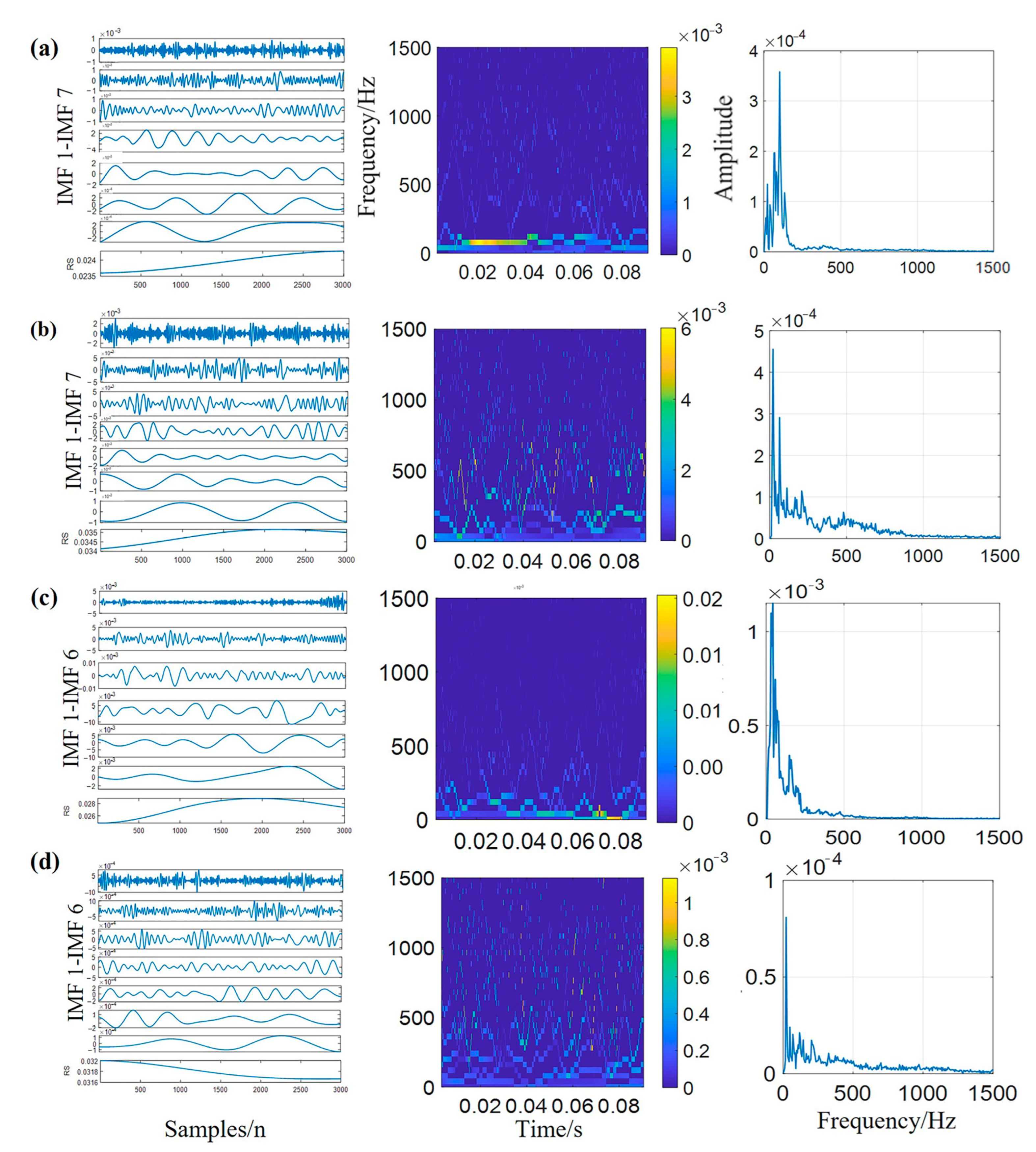
3.1.1. Multi-Scale Feature Extraction Method

Feature extraction is a critical component of the system to improve its generalization ability. It aims to extract various types of features that contain as much information as possible about the ship-radiated noise. However, due to the noise-like character in the power spectrum of ship-radiated noise, it is complicated to accurately obtain the character of the noise in its spectrum. Moreover, ship-radiated noise has a significantly wider frequency range that reflects noise characteristics in its spectrum. As a result, it is difficult to construct suitable filters to obtain powerful information and compress low-dimensional features from ship-radiated noise without any prior knowledge. Learnable amplitude–time–frequency features tend to include more comprehensive information, but a considerable portion is useless or conflicting. In this work, we experimentally evaluate HHT-based features. The following equation can be used to describe the observed signal:

$$x(t)=s(t)+n(t)\hspace{1em}\hspace{1em}t=1,\dots ,T,$$

(1)

where $x(t)$ is the original time domain ship-radiated noise, $s(t)$ represents the pure ship-radiated noise, and $n(t)$ denotes the natural noise. In practice, a hydrophone system can effectively focus on a valid signal $s(t)$ when the radiated noise is much greater than the background ambient noise. In feature extraction processing, it is simulated as pure ship-radiated noise because $s(t)$ is the main component. The ship-radiated noise signal is intercepted into samples with a length of 3000 sampling points.

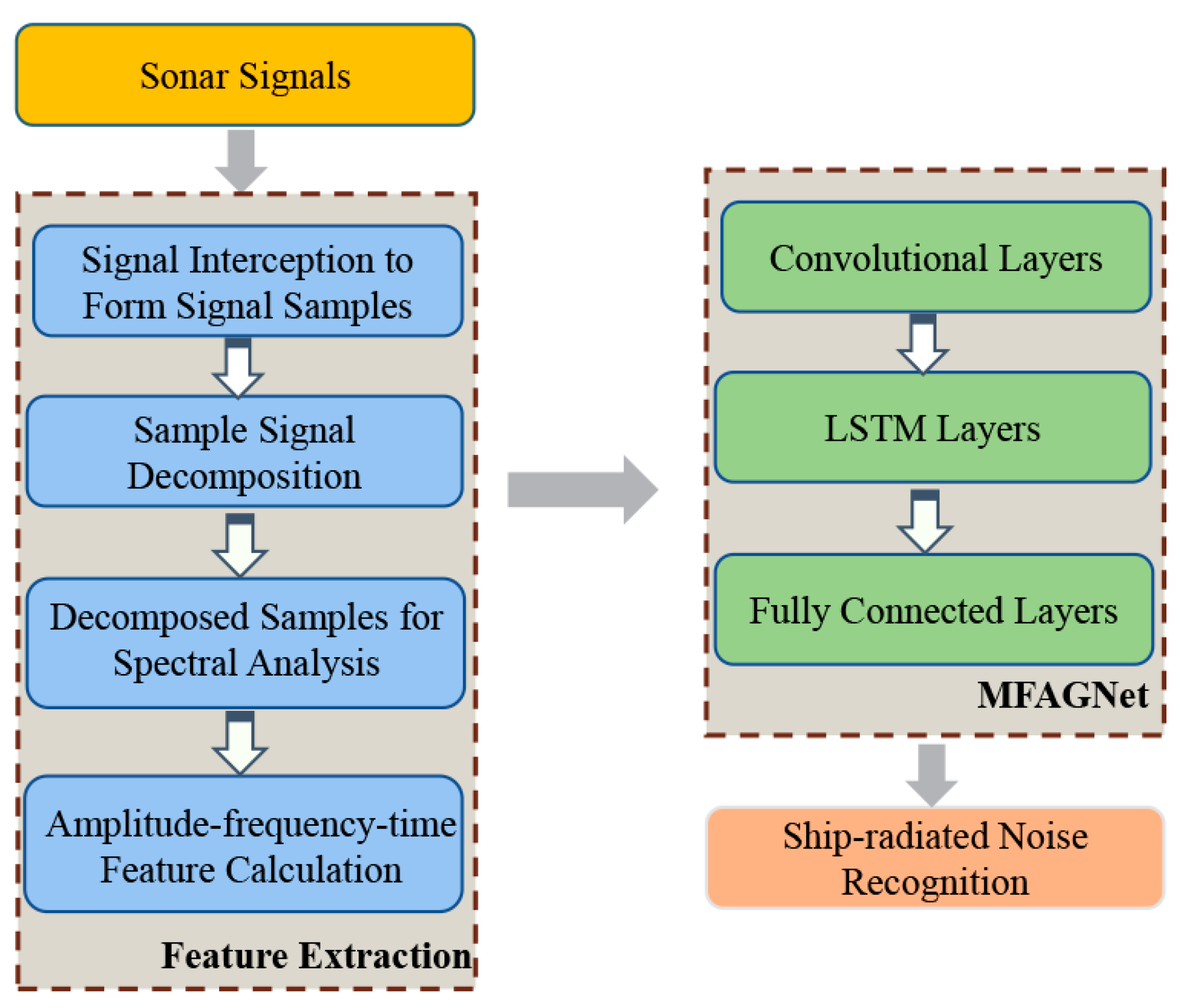
After improved HHT-based extraction algorithms, each intercepted sample is transformed into a feature matrix, which can be utilized by the following recognition system. The process of multi-scale feature extraction is illustrated in Figure 3. In this study, we extracted six representative features, which include energy, frequency and time domain amplitude. Features are extracted based on the explanation given below, and the resulting amplitude–time–frequency domain feature data are stored in the novel form of the feature matrix. These feature matrices serve as input to the proposed MFAGNet model, as well as machine learning and deep learning models applied for comparison in this study.

1.

Improved Hilbert-Huang transform algorithm

The Hilbert-Huang transform algorithm requires the following two steps: EMD and Hilbert spectrum analysis (HSA). The essence of the EMD algorithm decomposes any signal into a collection of the so-called intrinsic mode functions (IMFs) [38], and each of the IMFs is a narrow-band signal with a distinct instantaneous frequency that could be computed by using the HHT [39].

$$IM{F}_i={\alpha }_i(t)\cos (\int {\omega }_i(t)dt)\hspace{1em}\hspace{1em}(i=1,2,\dots ,n),$$

(2)

where $IM{F}_i$ represents oscillatory modes embedded in $x(t)$ with both amplitude ${\alpha }_i(t)$ and frequency and $f_i(t)={\omega }_i(t)/2\pi$. ${\omega }_i(t)$ is the instantaneous angular frequency. The instantaneous frequency extracts the frequency that varies with time from the signal.

Compared with signal processing methods that apply fixed basis functions, such as Fourier transform and wavelet transform, the EMD algorithm can intuitively, directly and adaptively decompose a given signal to a collection of IMFs. However, the ship-radiated noise consists of a broadband component, narrow-band spectral and random environment noise, so it has strong non-stationary non-linear characteristics. Traditional EMD methods are susceptible to mode aliasing when processing such signals, leading to the ineffective decomposition of signals. Therefore, the feature extraction process used an improved version of the traditional EMD algorithm named the MEEMD algorithm, which calculates the permutation entropy (PE) to eliminate false components in the signal, screens out the main IMF components, and then suppresses mode aliasing. Adaptive decomposition and the acquisition of effective IMFs can provide valuable information on the feature extraction and recognition of ship-radiated noises.

In this work, we utilize the improved Hilbert–Huang transform algorithm to achieve better feature extraction. At first, the Hilbert transform is carried out based on the decomposed signal. It is applied to calculate the instantaneous frequency of each order IMF, in order to gain the amplitude–time–frequency representation of the signal, namely the Hilbert spectrum. The Hilbert spectrum represents the distribution of instantaneous amplitudes in the frequency–time plane, with good time–frequency aggregation. Additionally, the Hilbert marginal spectrum is gained by calculating the integral of the Hilbert spectrum over the whole period, which demonstrates the distribution of the same frequency amplitude or energy superposition value in the frequency domain during the entire time–frequency range. The Hilbert spectrum and Hilbert marginal spectrum are expressed in Equations (3) and (4).

$$H(\omega ,t)=\mathrm{Re}{\displaystyle {\sum }_{i=1}^n{{\displaystyle a}}_i(t){{\displaystyle e}}^{i{\displaystyle \int {{\displaystyle \omega }}_i(t)dt}}},$$

(3)

$$\begin{array}{l}h(\omega )={\displaystyle {\int }_0^{T}H(\omega ,t)dt}={\displaystyle \sum _1^n{\displaystyle {\int }_0^T\mathrm{Re}\left({{\displaystyle a}}_i(t){{\displaystyle e}}^{i{\displaystyle \int {{\displaystyle \omega }}_i}(t)dt}\right)}dt},\\ ES(\omega )={\displaystyle {\int }_0^T{H}^2(\omega ,t)}dt\end{array},$$

(4)

where $H(\omega ,t)$ and $h(\omega )$ are the Hilbert spectrum and Hilbert marginal spectrum, respectively.

2.

Amplitude–time–frequency domain features

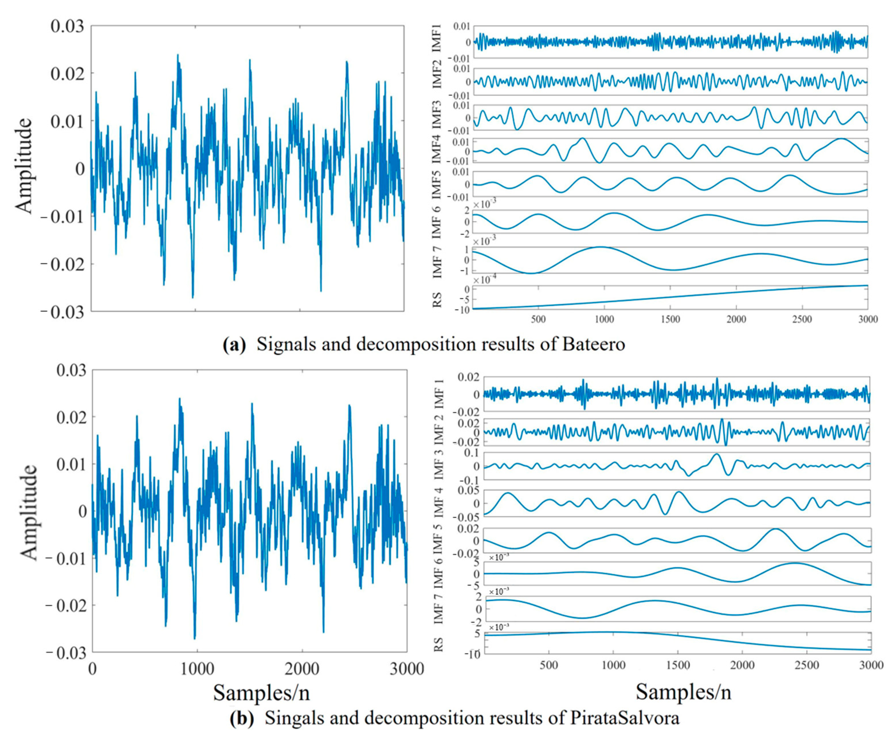
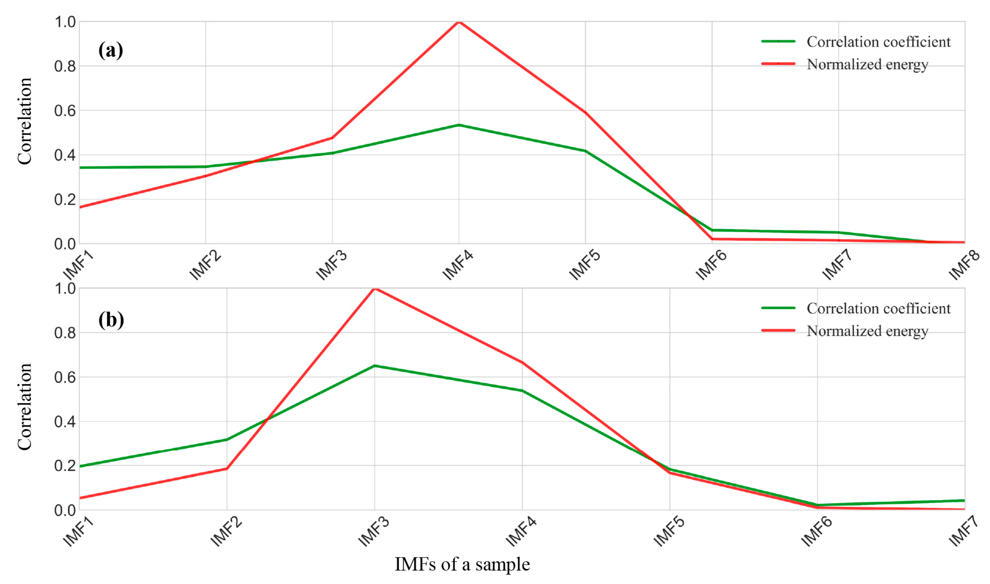
For sampled ship radiated noise, MEEMD will decompose these signals into a series of IMFs, including specific components. Once the sampled ship-radiated noise is decomposed, a sequence of IMFs can be obtained. However, direct observation of these IMF waves in the time domain still yields ambiguous results. Consequently, the first 6 IMFs that contain the main information, and the amplitude–time–frequency characteristic information is extracted by calculating the Hilbert–Huang spectrum and Hilbert marginal spectrum.

In the time domain, the Hilbert energy can be obtained by integrating the square of the Hilbert spectrum with time, which represents the energy accumulated by each frequency over the entire time length. It can be expressed as follows:

$$ES(\omega )={\int }_0^T{H}^2(\omega ,t)dt,$$

(5)

where $H(\omega ,t)$ represents Hilbert energy.

In the frequency domain, the Hilbert instantaneous energy spectrum can be obtained by integrating the frequency with the square of the Hilbert spectrum. Instantaneous energy represents the energy accumulated in the whole frequency domain at each time, and it can be expressed as follows:

$$IE(t)={\int }_{{{\displaystyle \omega }}_1}^{{{\displaystyle \omega }}_2}{H}^2(\omega ,t)d\omega ,$$

(6)

where $IE(t)$ represents the Hilbert instantaneous energy.

One can suppose that each IMF component contains N sampling points, and the instantaneous amplitude of the $n$th sampling point after Hilbert transform is denoted as ${{\displaystyle a}}_n$, and the instantaneous frequency is ${{\displaystyle f}}_n$. The instantaneous energy can be expressed as follows:

$$P_n=10\log Q_n,$$

(7)

where ${{\displaystyle Q}}_n={{\displaystyle a}}_n^2$. In the whole sampling time, the instantaneous energy variation range can be obtained as follows:

$$\Delta P=P_{\max }-P_{\min },$$

(8)

where any order of IMF energy $Q$ is defined as follows:

$$Q={\displaystyle {\sum }_{n=1}^N{{\displaystyle Q}}_n}$$

(9)

The average amplitude of any order of IMF ${{\displaystyle a}}_{mean}$ can be defined as follows:

$${{\displaystyle a}}_{mean}=\frac{1}{N}{\displaystyle {\sum }_{n=1}^N{{\displaystyle a}}_n}$$

(10)

In addition to the energy feature that can express noise information carried in the samples, the frequency feature is also essential to express the ship-radiated noise information of samples. The average instantaneous frequency of each order IMF is defined as follows:

$${{\displaystyle f}}_{mean}=\frac{1}{N}{\displaystyle {\sum }_{n=1}^N{{\displaystyle f}}_n},$$

(11)

The instantaneous frequency of any order of IMF always fluctuates around a central frequency, which is the central frequency of this order of IMF. Here, the IMF center frequency ${\widehat{f}}_{cfreq}$ of each order of IMF is defined as follows:

$${{\displaystyle \widehat{f}}}_{cfreq}=\frac{{\displaystyle {\sum }_{n=1}^N{{\displaystyle Q}}_n}{{\displaystyle f}}_n}{{\displaystyle {\sum }_{n=1}^N{{\displaystyle Q}}_n}}$$

(12)

because we select the first six-order IMFs and extract 6 amplitude–time–frequency representative features of each order of IMF, respectively. After extraction of the features, each sample is formed as a feature matrix with a dimension of 1 × 36.

3.1.2. The Proposed MFAGNet Model

For this system, the design of the recognition network is a crucial part. In this section, we describe the proposed MFAGNet network architecture in detail. Moreover, in addition to building high-performance networks, data preprocessing often plays an effective role in the effectiveness of the network. Therefore, taking into account the complex multi-scale features, the data preprocessing method is presented and described below.

1.

The architecture of MFAGNet

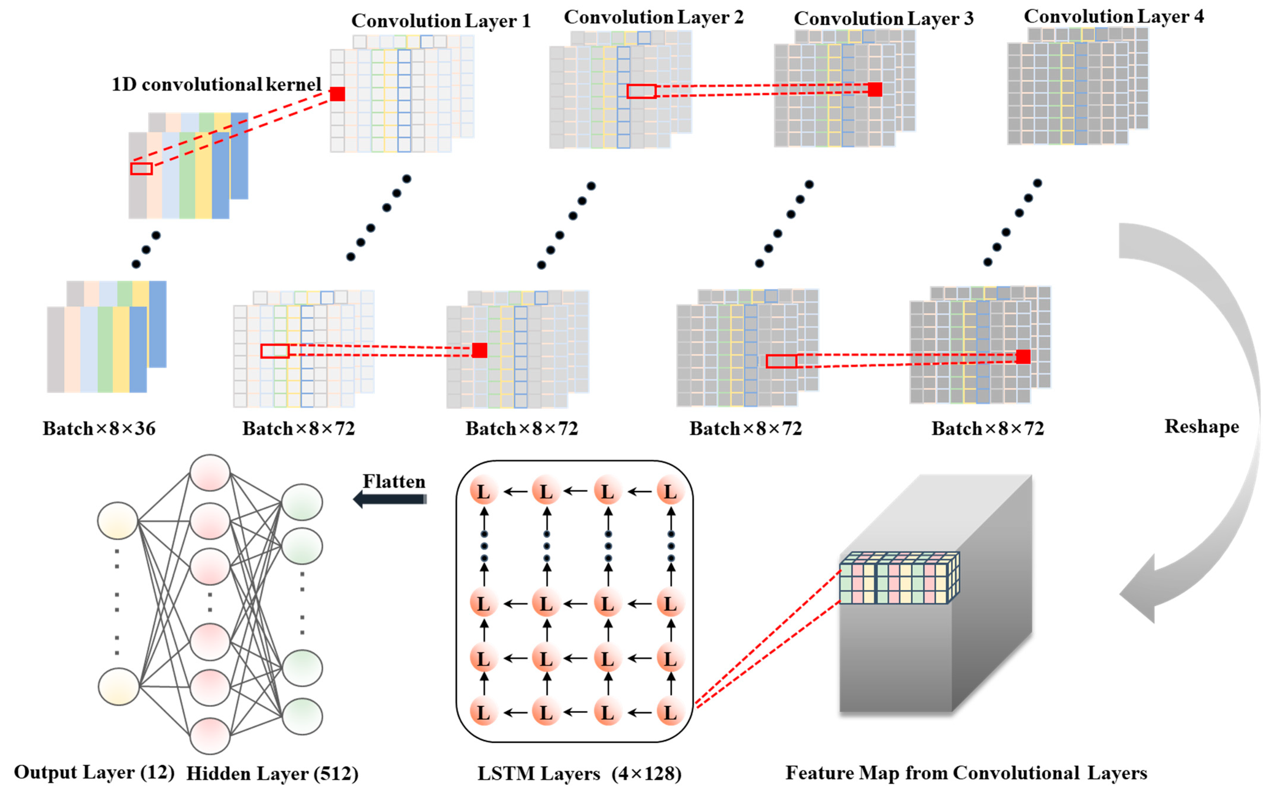
In order to enhance ship recognition performance, a new hybrid neural network termed MFAGNet is proposed, which primarily combines the CNN and LSTM according to the types of extracted feature matrices. Figure 4 shows the proposed neural network structure that contains various types of modules, such as multiple convolutional neural layers, recurrent layers, and fully connected layers. The key concept of MFAGNet is to better use feature matrices that have both spatial and temporal coupling characteristics as the basis for the samples. Applying these strategies to construct network models will considerably enhance the training efficiency of the neural network model and the accuracy of the recognition performance.

Convolutional neural networks are capable of learning not only image feature information but also sequence data, including various signal data, time series data, and natural language processing [40]. Taking into account the ability of 1D CNN to extract serial information features, 1D convolutional layers are applied as the shallow layer of MFAGNet. With this design approach, temporal information on the extracted features can be directly learned and enriched. Following multiple convolution layers, LSTM layers are employed as a second module to extract features at each time index. Eventually, the recognition results are outputted by fully connected layers.

(1)

Convolutional Layers:

Two-dimensional CNN architectures have traditionally been applied to image processes to extract detailed image information features. However, input feature matrices used in ship recognition are one-dimensional in nature, making them unsuitable for 2D and 3D CNN architectures. The 2D and 3D CNN architectures require data converted to image form, which leads to the loss of detailed information. In addition, the 1D CNN operation does not alter feature orders, greatly reducing the network complexity. Although it will reduce the number of training parameters, the pooling layer is still removed to prevent the loss of feature information.

MFAGNet contains four convolutional layers. Table 2 shows the size of the convolutional kernels and the layer number of filters in each convolutional layer, and Figure 4 displays the architecture of the convolutional layers. After conducting numerous experiments, it was found that the best convolutional structures are those with kernel sizes of 2 × 72, 2 × 72, 2 × 72, 2 × 72 and 2 × 72 for each layer. It is possible to enhance the ability of convolutional layers to extract multiple features. The output of each convolutional layer is taken as input to a batch normalization layer and a Randomized Leaky Rectified Linear Units (RReLU) layer. The operations are well defined by Equation (14).

$$z_j^k=f(BN({\displaystyle \sum }_i{z}_i^{k-1}\ast w_{ij}^k+b_j^k),$$

(13)

where $z_j^k$ is the $j$th feature map generated by the $k$th layer. $w_{ij}^k$ represents the weight associated with the $j$th convolution kernel and the $i$th feature map. BN signifies the batch normalization operation and $f()$ denotes the function of the activation we selected for each layer. $b_j^k$ is the bias concerned with the $j$th convolution kernel and $\ast$ means the convolution operation between the input feature map and the convolution kernel.

(2)

LSTM Layers:

As the input data have sequential characteristics, it is necessary to apply LSTM layers to extract features from the ship noise signals. The typical recurrent neural network (RNN) only has a chain structure of repetitive modules with a non-linear tanh function layer inside [41,42]. However, it is complicated for a basic RNN to learn complex non-linear features with this simple structure, and the training process is prone to gradient instability. In contrast, LSTM has a repeating module structure that is more elaborate and has an excellent capability to extract time series features [43]. It employs specialized hidden units that enable the retention of long-term memory, while mitigating the issue of gradient vanishing [44]. Therefore, LSTM is selected to design recurrent layers with the aim of extracting temporal features. LSTM can be mathematically represented by the following expressions.

Initially, the forget gate gating signal determines the discarded information in the cell state, as follows:

$$R_f=\sigma (W_f\ast {\left[h_{t-1},I{n}_t\right]}^T+b_f),$$

(14)

where $I{n}_t$ denotes the input data at the current moment, $W_f$ is the weight matrix of the forgot gate, $b_f$ represents the bias term and then the last moment state $h_{t-1}$ is multiplied by the weight matrix. $R_f$ indicates that the data are transformed to a number between 0 and 1 by the sigmoid activation function.

Then, the input gate determines the amount of information updated on the cell status. The input data go through the sigmoid activation function to create the updated candidate vectors. In addition, the calculation of the input gate is applied to decide which input data need to be updated, as follows:

$$R_i=\sigma (W_i\ast {\left[h_{t-1},I{n}_t\right]}^T+b_i),$$

(15)

$$R_c=\tan h(W_c\ast {\left[h_{t-1},I{n}_t\right]}^T+b_c),$$

(16)

where $R_i$ represents the state of the update gate and $R_c$ denotes the input node whose value between −1 and 1 passes through a tanh activation function. They work together to control the update of the cell state. The previous steps are combined with the forgetting gate to determine the update state. The old state $C_{t-1}$ is multiplied by $R_f$ and added together with the result of the input gate to decide the updated information. It can obtain the update state with the value $C_t$.

$$C_t=C_{t-1}\otimes R_f+R_c\oplus R_i,$$

(17)

where the output gate controls the next hidden gating state, and is determined by the following two parts: the first part is the output vector value generated by the updated cell state, while the second part is used to calculate the result of the gate state, which can be described as the following equations:

$$R_o=\sigma (W_o\ast {\left[h_{t-1},I{n}_t\right]}^T+b_o),$$

(18)

$$h_t=R_o\otimes \tan h(C_t),$$

(19)

where $R_o$ is the result of the output gate and it is calculated through the tanh activation function with $C_t$ to obtain the output data $h_t$. The combination of these different gate signals ensures that the information does not disappear owing to time lapse or extraneous interference.

The LSTM network layers contain four layers, and the input data are derived from the features obtained from the CNN layers. The first LSTM layer contains 128 cells, and the output dimension of all the other three LSTM layers is also 128. The effective features are extracted by four LSTM layers.

(3)

Fully connected layers:

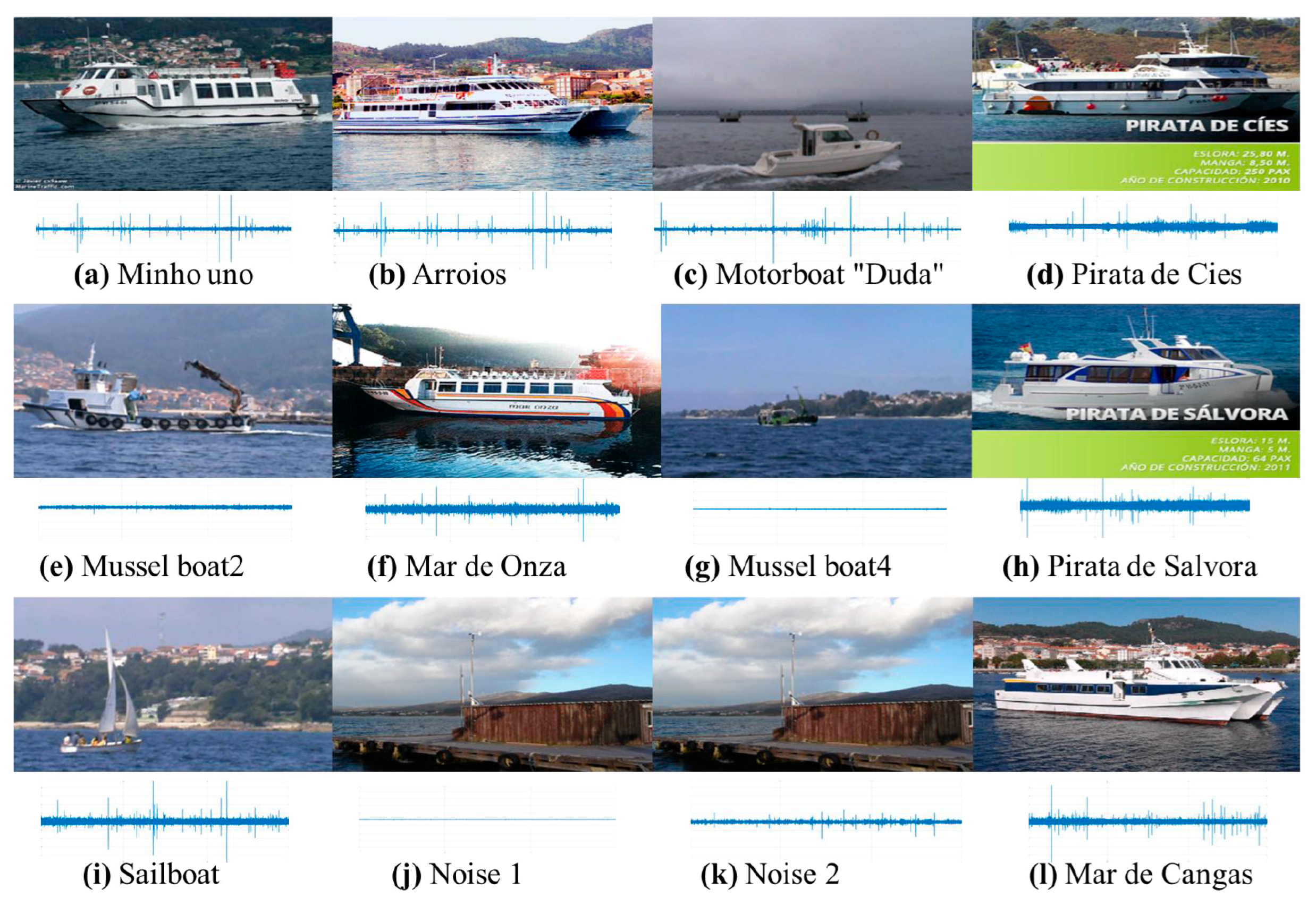
The fully connected layers in our proposed MFAGNet model consist of one hidden layer with 512 fully connected neurons. The output result layer has a total of 12 neurons, corresponding to the 12 specific noises. In this work, the feature map of the last time step in the final LSTM layer is selected to be inputted to the fully connected layer through a flattening operation. After the hidden layer and the dropout layer, the obtained feature extraction results are inputted into the Softmax layer for optimal classification results. The Softmax activation function can be described as follows:

$$\mathrm{Softmax}({\theta }_i)=\frac{e^{{\theta }_i}}{{{\displaystyle \sum }}_{n=1}^N{e}^{{\theta }_n}},$$

(20)

where ${\theta }_i$ represents the model parameters we obtained, and N denotes the total number of specific noises. The Softmax classifier calculates the probability of each class and normalizes all exponential probabilities. The highest prediction probability is chosen as the recognition result of the network.

Regarding the convolutional and hidden layers of the proposed network, the RReLU activation function is selected and described as follows:

$$\mathrm{R}\mathrm{R}\mathrm{e}\mathrm{L}\mathrm{U}\left(x\right)=\left\{\begin{array}{ll}x& if x\ge 0\\ \alpha x& otherwise\end{array}\right.,$$

(21)

where $\alpha$ is randomly sampled in the range [0.125, 0.25]. On the one hand, it has negative values, which allow gradients to be calculated in the negative part of the function. On the other hand, it can be set to a random number in this interval during the training and a fixed value during the testing. This design can effectively reduce the existence of dead neurons to learn gradients in the training.

Table 2. The architecture of MFAGNet.

Layer Type	Configuration
Convolutional Layers
Convolution 1D + BatchNorm	Filters: 2 × 72, RReLU
Convolution 1D + BatchNorm	Filters: 2 × 72, RReLU
Convolution 1D + BatchNorm	Filters: 2 × 72, RReLU
Convolution 1D + BatchNorm	Filters: 2 × 72, RReLU
LSTM Layers
LSTM + Dropout	Filters: 128, Tanh, 0.5
LSTM + Dropout	Filters: 128, Tanh, 0.5
LSTM + Dropout	Filters: 128, Tanh, 0.5
LSTM + Dropout	Filters: 128, Tanh, 0.5
Fully Connected Layers
Fully Connected + Dropout	Filters: 512, RReLU, 0.5
Output Layer	Filters: 12, RReLU

Table 2. The architecture of MFAGNet.

Layer Type	Configuration
Convolutional Layers
Convolution 1D + BatchNorm	Filters: 2 × 72, RReLU
Convolution 1D + BatchNorm	Filters: 2 × 72, RReLU
Convolution 1D + BatchNorm	Filters: 2 × 72, RReLU
Convolution 1D + BatchNorm	Filters: 2 × 72, RReLU
LSTM Layers
LSTM + Dropout	Filters: 128, Tanh, 0.5
LSTM + Dropout	Filters: 128, Tanh, 0.5
LSTM + Dropout	Filters: 128, Tanh, 0.5
LSTM + Dropout	Filters: 128, Tanh, 0.5
Fully Connected Layers
Fully Connected + Dropout	Filters: 512, RReLU, 0.5
Output Layer	Filters: 12, RReLU

A mini-batch gradient descent approach is employed to train the neural network and the training set is partitioned into multiple groups. The model achieves gradient updates at each mini-batch data iteration. The Softmax cross entropy as the loss function is adopted with the adaptive motion estimation (Adam) optimizer. During the training process, the main objective is to minimize the loss between the predicted values and the ground truth by utilizing the optimizer strategy. The loss function is given as follows:

$$L_{SCE}=-{\displaystyle \sum }_{i=1}^m\log \frac{e^{W_{y_i}^T{x}_i+b_{y_i}}}{{{\displaystyle \sum }}_{j=1}^n{e}^{W_j^T{x}_i+b_j}}$$

(22)

where $n$ represents the total number of classes and neurons in the output layer. $m$ indicates batch size. $x_i$ denotes the hidden features of the $i$th sample. $y_i$ is the ground truth label of $x_i$. $W_j$ is the weight matrix of class $j$ and $b_j^{}$ represents the bias term. Through multiple rounds of parameter tuning experiments, MFAGNet is selected as the optimal parameter configuration. 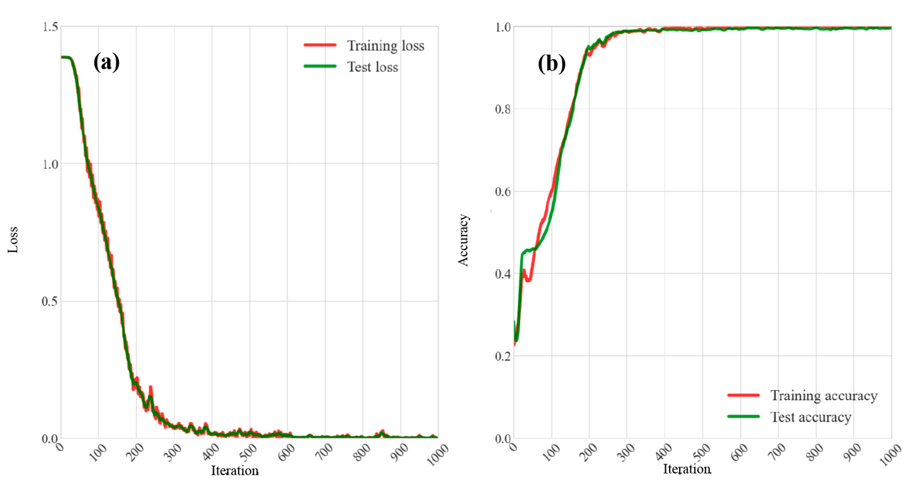The learning rate of the model is set at 1 × 10⁻⁴, while the batch size is set to 128 and the dropout parameter is set to 0.5. The model is trained for 1000 epochs on two 3090 Ti GPUs, and the best-performing model based on classification accuracy is selected.

3.2. Evaluation Metrics

For all experiments, the four classical and effective metrics are widely applied to evaluate algorithms, such as accuracy, precision, recall and F1-score. Accuracy can be described as the rates of correctly classified samples among all samples, which is expressed by the following expression:

$$\mathrm{Accuracy}=\frac{TP+TN}{TP+TN+FP+FN},$$

(23)

where TP denotes true positive, FP represents false positive, TN is true negative, and FN means false negative. Assessment only based on accuracy may significantly influence the evaluation results when unbalanced datasets are encountered. In order to overcome this problem, the model needs to be evaluated with other classical metrics that are given as follows:

$$\mathrm{Precision}=\frac{TP}{TP+FP},$$

(24)

$$\mathrm{Recall}=\frac{TP}{TP+FN},$$

(25)

$$\mathrm{F}1-\mathrm{score}=2\ast \frac{ \mathrm{Precision}\ast \mathrm{Recall}}{ \mathrm{Precision}+\mathrm{Recall}},$$

(26)

4. Results and Discussion

4.1. Analysis of Ship-Radiated Noise and Multi-Scale Features

Figure 5 depicts the original ship-radiated noise samples of 3000 sampling points. Figure 5a illustrates the original sampled ship-radiated noise of Bateero and its decomposition results, while Figure 5b presents the original sampled ship-radiated noise of PirataSalvora and its decomposition results. The sample signals of both types of ship-radiated noise are decomposed into a series of sub-signals, ranging from high frequency to low frequency. The first six-order sub-signals, namely IMF1-IMF6, make up the majority of the original signal. Therefore, the first six-order signal components are selected to be utilized.

In Figure 6a, the sampled radiated noise frequency of Bateero is mainly concentrated below 1000 Hz, with almost no frequency distribution in the 1000–4000 Hz frequency band. Moreover, it can be observed more clearly from the marginal spectrum that the frequency is mainly concentrated on the 0–500 Hz frequency band. The analysis results indicate that the effective information of the Bateero’s radiate noise is mainly concentrated on the 0–500 Hz frequency band, while the high frequency, especially the 1000–4000 Hz frequency band, contains almost no effective information extraction. Figure 6b displays the Hilbert–Huang spectrum and marginal spectrum of PirataSalvora’s radiated noise sample. Similar to Figure 6a, the main information of this ship-radiated noise sample is concentrated below 500 Hz, but with a slightly different specific frequency distribution. Therefore, it is challenging to extract effective features that distinguish between ship-radiated noise with similar frequency distributions by single features such as frequency features. The extraction of multi-dimensional and multi-type features is crucial for the accurate recognition of the following systems.

Different ship-radiated noise, as well as different samples of the same ship-radiated noise, can result in different numbers of IMF components during decomposition. Therefore, it is crucial to measure the proportion of each order of IMF component in the entire original signal to select effective components. Figure 7 displays the correlation coefficients between IMFs and the original sampled signal, as well as the normalized energy of IMFs. Figure 7a demonstrates that the radiated noise sample of Bateero is decomposed into 8-order IMF components, where IMF 4 has the highest correlation coefficient with the original sample noise signal and occupies the most energy. The figure also demonstrates that the energy of the first six-order IMF components almost completely occupies the whole original signal, which further proves that selecting the first six-order IMF components for feature extraction is effective. Figure 7b illustrates the correlation coefficients and normalized energy of each order of IMF and the original signal of the radiated noise samples from PirataSalvora, where IMF 3 demonstrates the highest capacity and has the highest correlation coefficient. Similarly, the first six-order IMF components can almost express the information of the entire original sample signal. Therefore, as representative feature information, energy can be extracted by improved HHT-based methods to obtain another type of feature information.

In addition to extracting multi-dimensional and multi-type features, the combination of features plays a key role in effective ship recognition. Therefore, after using complete 6-type features for ship recognition experiments, different combinations according to the properties of the features are made to verify the sensitivity of the recognition system. Six different combinations of energy-based, amplitude- and frequency-based features are applied for comparison, specifically including combination A (all six features), combination B (instantaneous energy variation range and IMFs-Energy), combination C (IMFs-Center frequency and IMFs-Average amplitude), combination D (IMFs-Average amplitude and IMFs-Average frequency), combination E (Instantaneous energy variation range, IMFs-Center frequency and IMFs-Average amplitude) and combination F (IMFs-Center frequency, IMFs-Center frequency2, IMFs-Average amplitude and IMFs-Average frequency).

4.2. Comparison between MFAGNet and Other Models

4.2.1. Effective Evaluation of MFAGNet

In this work, 70% of the data are randomly divided into a training set and 30% of the data are randomly designated as the test set in all models. The original ship noise is transformed into amplitude–time–frequency feature matrices by utilizing the multi-scale feature extraction method. Next, the preprocessing procedure involves mainly normalization of the multi-scale features, which are reshaped to resemble a sequence in a specific form. The sample feature matrices are scaled by using the normalization algorithm to map the trainable feature matrices to the range of [0, 1]. The normalization algorithm can be expressed as follows:

$$F^{’}=\frac{F-min}{max-min},$$

(27)

where $F$ represents the data of original features with 5879 sample, where each dimension is 1 × 36, and $F^{’}$ represents the data of normalized features. The max and min in the normalization algorithm represent the maximum and minimum values of all features, respectively. After muti-scale feature data are normalized, the resulting current features coupled with extracted features of the next 7 time steps are taken as input data for each step of the MFAGNet model. It is noted that each feature data sample has 8 time steps, which are converted into 2D data with a size of 8 × 36, as shown in Figure 4.

Four machine learning methods and three deep learning methods widely applied in the fields of ship recognition are chosen for comparison with the proposed MFAGNet model. The comparison aims to validate the effectiveness of the proposed MFAGNet model. Various machine learning-based models are selected for comparison, such as the KNN, SVM, naive Bayes (NB) and RF, which have been previously adopted in the recognition of underwater acoustic data with certain effectiveness [16]. At the same time, deep learning-based architectures have also made great progress in this area, including CNNs, LSTMs and deep neural networks (DNNs) [29]. By setting parameters and controlling variables, we apply these models to compare the recognition results. Descriptions are listed in the following sections.

CNNs: A sequence CNN model is designed to contain a stack of 1D CNN layers, batch normalization layers, and fully connected layers with the RReLU activation function. The data flow through the pipeline as if the output of the previous layer is the input of the following layer. Four 1D CNNs layers with a size of 2 × 72 filters are set up, including a batch normalization layer. The results are input into two fully connected layers with nodes 512 and 12, including a dropout layer. The same convolutional layer parameters and fully connected layer parameters are chosen to compare with MFAGNet to verify the effect, such as the same parameter settings, loss function and so on. The detailed architecture is shown in

Table 3. The architecture of CNNs.

Layer Type	Configuration
Convolutional Layers
Convolution 1D + BatchNorm	Filters: 2 × 72, RReLU
Convolution 1D + BatchNorm	Filters: 2 × 72, RReLU
Convolution 1D + BatchNorm	Filters: 2 × 72, RReLU
Convolution 1D + BatchNorm	Filters: 2 × 72, RReLU
Fully Connected Layers
Fully Connected + Dropout	Filters: 512, RReLU, 0.5
Output Layer	Filters: 12, RReLU

.

LSTMs: A designed LSTM-based architecture contains LSTM layers, dropout layers and fully connected layers. It is compared with our proposed model to achieve the ship noise classification mission. As shown in

Table 4. The architecture of LSTMs.

Layer Type	Configuration
LSTM Layers
LSTM + Dropout	Filters: 128, Tanh, 0.5
LSTM + Dropout	Filters: 128, Tanh, 0.5
LSTM + Dropout	Filters: 128, Tanh, 0.5
LSTM + Dropout	Filters: 128, Tanh, 0.5
Fully Connected Layers
Fully Connected + Dropout	Filters: 512, RReLU, 0.5
Output Layer	Filters: 12, RReLU

, four LSTM layers mainly extract feature information from time series and iterate continuously in the sequence form, accompanying dropout layers reported with the same shape of 128 cells. Two fully connected layers are added to perform the classification task, with 512 and 12 neurons, respectively.

DNNs: For comparison, the complex architecture of DNNs comprising 5 layers with the number of nodes 245, 512, 512, 256 and 12 (the total number of ship noise classes) is built. The same activation function RReLU is applied, and the parameters of the dropout layer are set to the same values.

Table 5. The architecture of DNNs.

Layer Type	Configuration
Fully Connected Layers
Fully Connected + Dropout	Filters: 256, RReLU, 0.5
Fully Connected + Dropout	Filters: 512, RReLU, 0.5
Fully Connected + Dropout	Filters: 512, RReLU, 0.5
Fully Connected + Dropout	Filters: 256, RReLU, 0.5
Output Layer	Filters: 12, RReLU

illustrates the detailed architecture of the DNNs.

Machine learning methods: Compared to deep learning methods, the four machine learning methods have relatively simpler parameters. Firstly, the KNN algorithm is tested through experiments to determine the optimal parameter of neighbors, which is found to be 8. Next, the SVM is trained with a regularization parameter of 0.5 with the linear kernel. Then, NB is used with a default prior probability. Finally, RF is trained with 200 estimators.

The processes of training the proposed MFAGNet and LSTMs models by using combination A are illustrated in Figure 8, which records the evolution of accuracy and loss in detail. The parameter of the initial learning rate is set to 0.001 and decays automatically as the number of iterations changes. The models are trained with 1000 iterations, and the training loss and test loss of MFAGNet gradually decrease towards 0 with an increasing number of epochs in Figure 8a. The model effectively learns the underlying features of the data without incurring the issue of overfitting. Furthermore, the accuracy of both the training and testing sets improves steadily, eventually reaching values close to 1 during the training process. These demonstrate that MFAGNet has already reached its learning capacity limit.

Multiple models are compared using the same feature combination, while the same model is trained with different feature combinations. A total of six feature combinations are used to train eight algorithm models, resulting in the generation of forty-eight different models. Due to space limitations, only the training process of LSTMs trained with a combination A is presented in this article, while the rest is not displayed. Figure 8b illustrates the loss and accuracy score over time with the LSTM architecture, which was trained by setting the same parameters as the MFAGNet model. In comparison to MFAGNet, the training loss is less smooth, with larger differences between the test loss in LSTMs. Furthermore, the test accuracy indicates little overfitting and only achieves 93.19%, as shown in Table 3. The training process and results of the other models are similar to those of LSTMs, indicating that our proposed MFAGNet model demonstrates high effectiveness in both the training and results.

The confusion matrix as shown in Figure 9 illustrates the effectiveness of the proposed MFAGNet model in recognizing the test data, by using combination A. The rows of the matrix represent the predicted 12 specific noises, and the columns correspond to the true 12 specific noises. Each cell contains the number of observations and the proportion of all observations. The diagonal elements represent the accurately classified observations and the off-diagonal cells indicate misclassified observations. The rightmost column displays the percentages of all instances accurately and inaccurately classified for each ship class, where the green number represents the precision, and the red number denotes the false discovery rate. The last row of the figure presents the percentages of correctly and incorrectly recognized instances from each sound recording, the green number indicates the recall, and the red number is the false negative rate. In summary, the green diagonal cells represent instances for each ship class and their proportions for all samples. The red cells indicate the number and proportion of misclassified ships for each class.

The MFAGNet model achieves a total accuracy of 98.9%, as shown in the bottom-right cell of the confusion matrix. The ship recognition system exhibits outstanding performance in recognizing 12 complex specific noises, with an accuracy rate that is close to 100.0%. Each recording consists of approximately 100 samples, and the MFAGNet model demonstrates remarkable accuracy in classifying each class. It effectively distinguishes between various underwater ship-radiated noises and accurately recognizes ambient noise. However, the recognizer of Arroios has a relatively lower precision of 94.1%, leading to a relatively higher false negative rate of Pirata de Cies up to 5.1%. These belong to the passengers category, and their radiated noises have similar characteristics, which may account for the poor recognition effect. Therefore, how to accurately identify different ships of the same type using effect features is a valuable but challenging research direction.

The accuracy results of various methods using combination A extraction parameters are elaborated in

Table 6. Recognition accuracy (%) of combination A.

Method	Accuracy	Precision	Recall	F1-Score
MFAGNet	98.89	98.90	98.91	98.90
CNNs	92.68	92.67	93.45	92.76
LSTMs	93.19	93.21	94.28	93.12
DNNs	84.18	84.19	84.35	83.96
KNN	82.68	82.93	83.45	82.92
SVM	85.69	86.00	86.11	85.96
NB	79.49	79.88	79.33	79.35
RF	79.66	79.85	79.82	79.68

. Combination A includes all extracted features in the amplitude–frequency–time domain and is the most comprehensive feature combination. The results demonstrate that the proposed MFAGNet model achieves an accuracy of 98.89%, which is superior to all other methods. In addition, the overall precision, recall and F1-score are 98.90%, 98.91% and 98.90%, respectively, indicating its superior effectiveness over others. The LSTM method outperforms other methods, with an accuracy of 93.19%, while achieving precision, recall, and F1-Scores of 93.21%, 94.28%, and 93.12%, respectively. The method that relies on DNNs only performs the worst, with accuracy, precision, recall, and F1-score values that are significantly lower than other deep learning methods. Among the machine learning methods, the SVM method has higher scores than other methods, with scores of 85.69%, 86.00%, 86.11% and 85.96%, respectively. The KNN method ranks second, achieving an accuracy of 82.68%. These results demonstrate that the proposed MFAGNet is better than other deep learning methods and machine learning methods. In addition, when using all feature combinations, these deep learning and traditional machine learning methods yield satisfactory recognition results, further confirming the effectiveness of multi-dimensional and multi-type feature extraction methods. Note that the results with other feature combinations are not shown here due to their lower performances than those obtained with all six features. From the overall results, it can be concluded that combination A is the most effective feature combination method and is the optimal choice as input for the deep learning model. Furthermore, MFAGNet achieves better accuracy than the other methods in terms of recognition performance. These results demonstrate the satisfactory recognition ability for 12 different complex noises, including ship-radiated noise and ambient noise. Our proposed method is capable of identifying specific ships, rather than only the types of ships.

4.2.2. Robustness Test and Application

It is widely acknowledged that the marine environment and weather exhibit intricate and dynamic characteristics in diverse ocean areas and under varying climatic conditions, which result in different impacts on the ship radiated noise. MFAGNet has demonstrated the precise identification of specific vessels, indicating the potential for superior classification performance of the ship type. Consequently, to establish the universality and effectiveness of MFAGNet, noise data of four ship types under distinct climatic conditions and from disparate data sets, which are different from the previous training data sets (ShipsEar), are randomly selected for comparison. The noise data used for the application are sourced from the DeepShip dataset [22], which is available for free download at https://github.com/irfankamboh/DeepShip and accessed on 21 May 2021. A part of the dataset with four different types of ships is utilized, namely cargo, tug, tanker and passenger ships, respectively. For each ship type, the sampling rate is 32 kHz and a truncation of about 0.1 s is applied as one intercepted signal. The used dataset generates close to 4000 samples in the form of a feature matrix for training and testing. Afterward, the 4000 feature matrix samples are randomly shuffled as an experimental data set, with 70% selected as the training set and the remaining 30% chosen as the test set to evaluate the effectiveness of the ship recognition system. Finally, the output layer of MFAGNet is modified to four neurons corresponding to the four types of ships classified. The additional parameters employed during model training are consistent with those utilized in the previous training session by using combination A, which is the optimal feature combination selected with the highest accuracy.

Figure 10 illustrates that the four types of ship noise we chose are random, unordered, and without any obvious regularity, suggesting that they are not intentionally selected to achieve a better recognition effect. Figure 11 displays the MEEMD decomposition results, Hilbert–Huang spectrum and marginal spectrum of different ship samples and it can be observed from this figure that the MEEMD method can effectively decompose the ship’s radiation noise signals, and the decomposition results exhibit no obvious modal aliasing, which is consistent with the experimental results from the ShipsEar database and the practicality of this decomposition method for highly non-stationary and non-linear ship radiated noise is once again verified. From the Hilbert–Huang spectrum and marginal spectrum of the four-type ship signals, there are significant differences in the spectrograms, which indicates that the frequency information contains characteristic information that can express a specific type of ship. Therefore, the use of features including frequency information is the key to obtaining high-accuracy classification. The form of the multi-scale and multi-dimensional feature matrix used in this study enables a more complete and comprehensive extraction of effective information from the time domain to the frequency domain, which provides sufficient guarantees for the high-performance network to achieve accurate classification.

Next, the t-distributed stochastic neighbor embedding (t-SNE) algorithm [45] is a statistical approach that allocates a position in a two or three-dimensional figure for showing high-dimensional data. Depending on the T-SNE method, Figure 12 presents the 3D visualization results of multi-scale features obtained by the improved HHT method in the feature space. The test dataset is utilized to construct it, where each color represents a different type of ship. In the three-dimensional feature space, it can be observed that ships of the same type cluster together, indicating that extracted multi-scale features have a favorable effect. Although feature extraction plays an important role in dimensionality reduction, there are still some limitations in which a part of data features is difficult to distinguish. Therefore, our proposed MFAGNet model extracts the potential features in high-dimensional feature space and attempts to achieve better accuracy.

Figure 13 visualizes the MFAGNet training process by using combination A, demonstrating the remarkable learning ability of the new dataset. It is evident that MFAGNet achieves fast convergence and satisfactory loss and accuracy.

Table 7. Recognition accuracy (%) of combination A with the new dataset.

Type of Noise	Accuracy	Precision	Recall	F1-Score
Cargo	98.90	99.32	97.35	98.33
Passenger Ship		98.98	100	99.49
Tanker		98.31	100	99.15
Tug		98.96	98.29	98.63

presents the identification results in the test data, achieving an overall accuracy of 98.90%, which is an outstanding performance. Each type of ship achieves an excellent recognition rate on almost 300 test samples. As expected, due to the classification task being simpler than the ship-specific recognition task, the proposed system can achieve high accuracy in classifying the type of ships. Our fine-grained ship-radiated noise recognition system exhibits satisfactory universality in the different datasets, as it effectively recognizes the types of ship noise in complex and varied marine environments through feature extraction and MFAGNet. These underscore the robustness and adaptability of our approach to overcoming environmental challenges and achieving excellent performance in various ocean conditions.

5. Conclusions

In this work, a fine-grained ship-radiated noise recognition system, which has consistently remained a focal point in maritime monitoring and vessel identification, is proposed and utilized in the field of underwater acoustics. It utilizes amplitude–time–frequency domain features obtained by the improved HHT method and the high-performance MFAGNet is proposed for recognition, achieving an excellent recognition accuracy of 98.89% for 12 specific complex sound recordings that include different specific ships and varying levels of ambient noise instead of just the type of ships. To investigate the applicability of the proposed method, we have utilized it in another public database, namely DeepShip, and selected four different types of ship noise for recognition. Afterwards, the same analysis method is applied, and there is no doubt that the task of ship classification is simpler compared to recognizing specific ships with a satisfactory accuracy of 98.90%. The experiment verifies the robustness and applicability of the proposed method. The main conclusions are as follows:

• A form of feature matrix is proposed for the first time, which adopts the improved HHT-based method to extract the energy, frequency and time domain amplitude features from the original ship-radiated noise.
• MFAGNet, a proposed spatio-temporal model, combines the significant advantages of LSTM and the spatial learning capability of the CNN to compensate for the inadequacies of the feature extraction of higher dimensional spaces. It obtains the best recognition accuracy and generalization for the different specific ships instead of just the type of ships.
• The proposed model is compared with other deep learning and machine learning methods by utilizing six different multi-scale feature combinations, achieving the highest accuracy for 12 specific noises. A total of 48 different models have been generated for comparison. In order to verify the universality and robustness with other datasets, experiments have been conducted, which also demonstrate excellent accuracy.
• The proposed method could automatically learn and update variables based on the data, eliminating the need for researchers to repeatedly tune various parameters. This end-to-end architecture can reduce the time required for deployment and decreases the probability of module docking issues, making actual deployment less troublesome.

The proposed system can effectively monitor maritime traffic and recognize the specific source of noise in the marine environment. However, it should be noted that the dataset used in this study is limited and the algorithm requires prior knowledge, which may not be convenient in practical applications. Next, in the face of more intricate and diverse specific ship noises, our method’s performance may be inadequate due to the inherent limitations of the model’s learning capacity. In addition, the specific multi-class ship noise model with strong noise resistance requires further exploration, which is one of our limitations. In the future, we will decrease, as much as possible, the complexity of our model to match the real-time needs of ship recognition and explore the ability to process more complicated data and tasks.