Holistic Reduction to Compare and Create New Indices for Global Inter-Seasonal Monitoring: Case Study for High Resolution Surface Water Mapping
Abstract
1. Introduction
- (1)
- A new globally applicable multispectral index for mapping and monitoring surface water extent that is able to include all the expressions of water regardless of turbidity across all seasons.
- (2)
- A new index with the same capabilities for sensors limited to the visible and NIR bands for local and retrospective monitoring of surface water extent at the highest possible resolution.
2. Methods
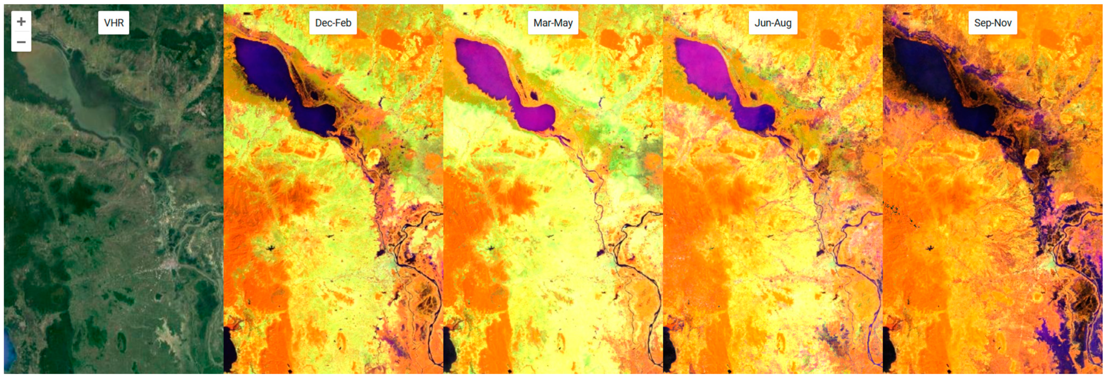
2.1. Understanding Temporal Variability via Visualization
2.2. Analysis Design
2.3. Study Areas
2.4. Imagery Preparation
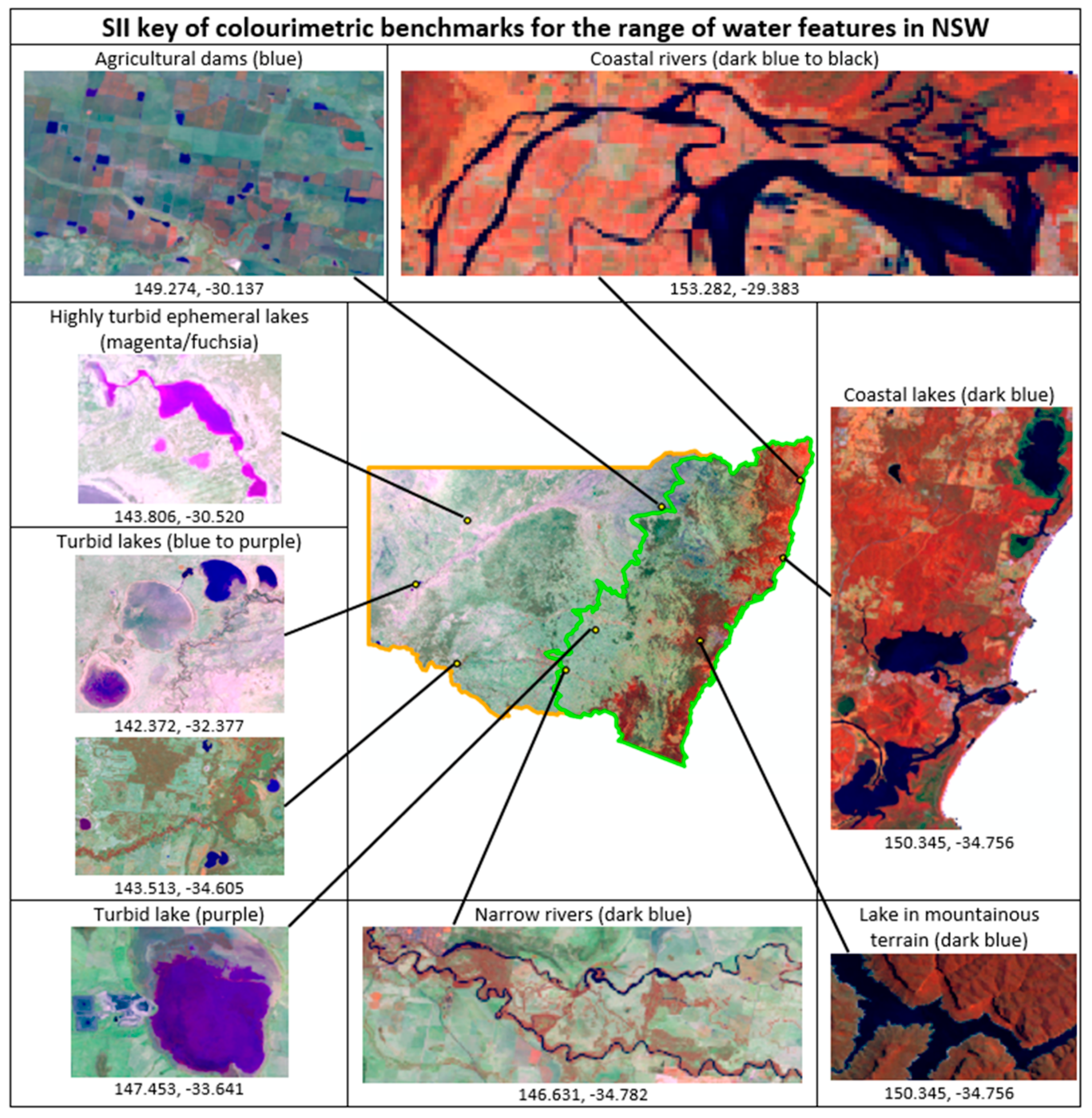
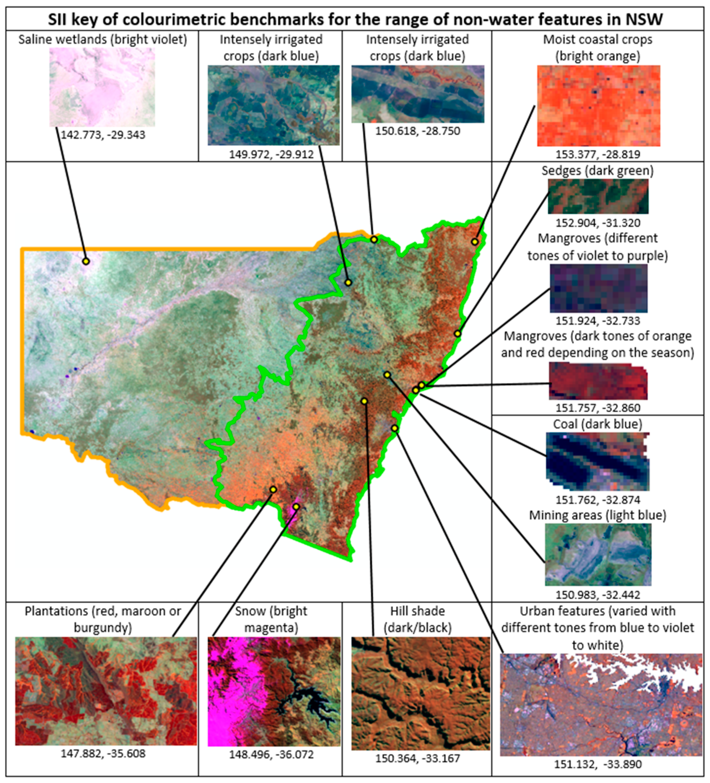
2.5. Satellite Imagery Interpretation Key with Colourimetric Benchmarks
2.6. Creation of the New Water Indices Presented in This Study
| Index | Equation | |
|---|---|---|
| Indices requiring SWIR bands | CHI | (Green − SWIR2)/NIR |
| CAWI | Log10 (Green/SWIR2/NIR) | |
| CWI | R,G,B: SWIR2, NIR, Green → H,S,V: Hue and Saturation | |
| Indices limited to the visible and NIR bands | CATWIC (combination of HRCWI and SR) | Where HRCWI = (Green − Red)/NIR and SR = Red/NIR |
| CHRWI | R,G,B: Red, (NIR + Blue)/2, Green → H,S,V: Hue | |
| BRCHRWI | R,G,B: Red/NIR, Blue/Green, Green/NIR → H,S,V: Hue | |
| NDCHRWI | R,G,B: ((Red − NIR)/(Red + NIR)) + 1, ((Blue − Green)/(Blue + Green)) + 1, ((Green − NIR)/(Green + NIR)) + 1 → H,S,V: Hue |
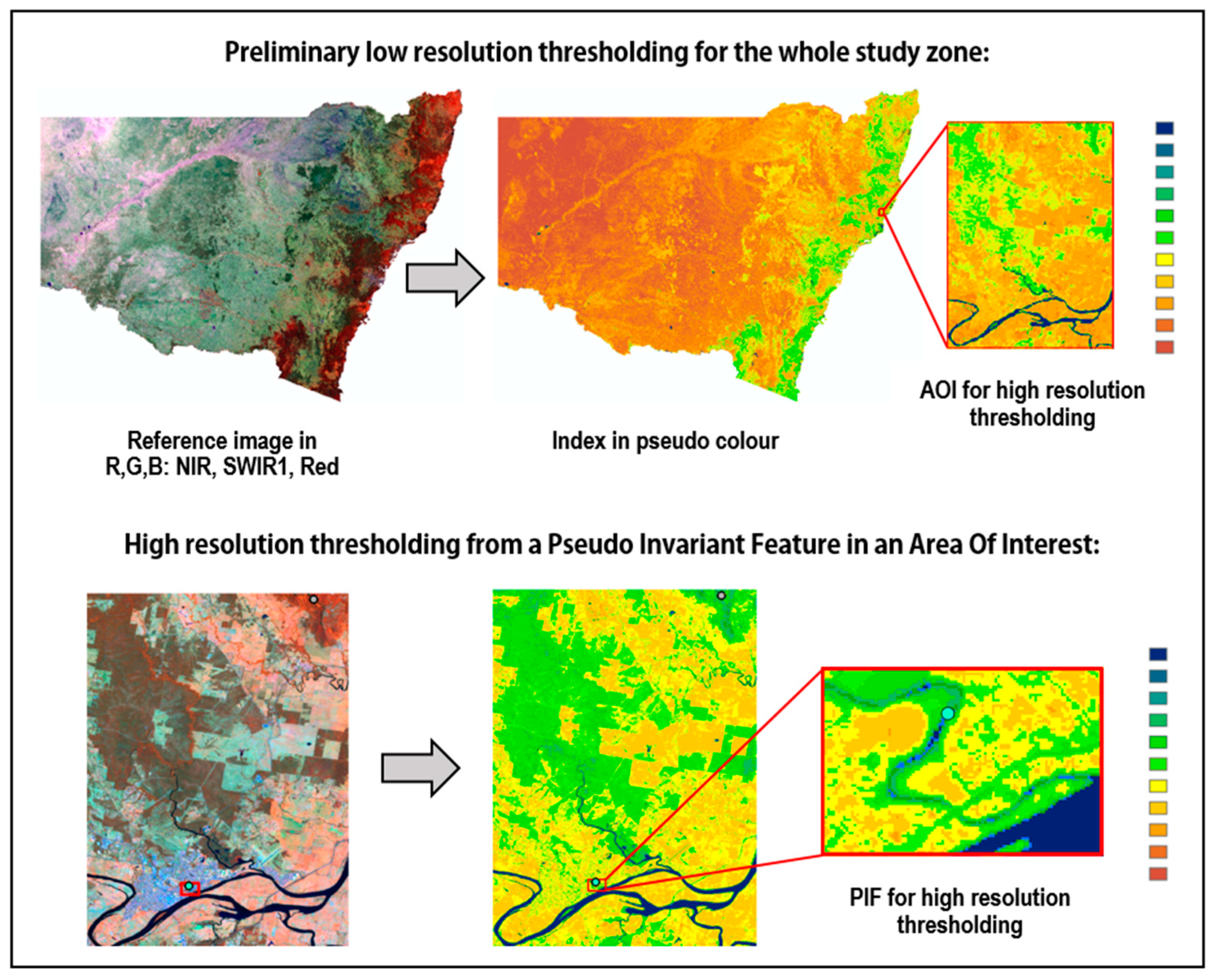
2.7. Threshold Determination for Indices and Their Comparison in the Decision Matrix
2.8. Development of Indices to Reduce Misclassification of Hill Shade, Urban Areas, Dry Salt Lakes, and Snow
- (1)
- Range: Max(R,G,B) − Min(R,G,B)
- (2)
- Simple ratio: Min(R,G,B)/Max(R,G,B)
- (3)
- Normalized difference ratio: (Max(R,G,B) − Min(R,G,B))/(Max(R,G,B) − Min(R,G,B))
- (4)
- Saturation of four bands: (Max(R,G,B,NIR) − Min(R,G,B,NIR))/Max(R,G,B,NIR)
3. Results
3.1. Phase 1—Comparison of Existing and New Indices with a Decision Matrix
3.2. Phase 2—Assessment of Best Performing Indices in Wetland, Agricultural, and Urban Environments
3.2.1. A Coastal Wetland Area
3.2.2. An Arid Wetland Area
3.2.3. An Intensely Irrigated Agricultural Area
3.2.4. A Complex Urban Area
3.3. Phase 3—Accuracy Assessment
3.4. Phase 4—Validation of the Selected Indices’ Performances across the Seasons and around the World
Comparison of Atmospheric Effects
4. Discussion
5. Conclusions
Supplementary Materials
Author Contributions
Funding
Data Availability Statement
Conflicts of Interest
References
- Willaarts, B.A.; Garrido, A.; Llamas, M.R. Water for Food Security and Well-Being in Latin America and the Caribbean: Social and Environmental Implications for a Globalized Economy; Routledge: London, UK, 2014. [Google Scholar]
- FAO; IFAD; UNICEF; WFP; WHO. The State of Food Security and Nutrition in the World 2022. Repurposing Food and Agricultural Policies to Make Healthy Diets More Affordable; FAO: Rome, Italy, 2022. [Google Scholar]
- Bhattacharya, S.; Banerjee, A. Water privatization in developing countries: Principles, implementations and socio-economic consequences. World Sci. News 2015, 10, 17–31. [Google Scholar]
- Arango, J.H.; Frutos, J.A.S.-D.; Molina, E.H. Murky waters: The impact of privatizing water use on environmental degradation and the exclusion of local communities in the Caribbean. Int. J. Water Resour. Dev. 2021, 38, 152–172. [Google Scholar] [CrossRef]
- Palmer, S.C.J.; Kutser, T.; Hunter, P.D. Remote sensing of inland waters: Challenges, progress and future directions. Remote Sens. Environ. 2015, 157, 1–8. [Google Scholar] [CrossRef]
- Pekel, J.-F.; Cottam, A.; Gorelick, N.; Belward, A.S. High-resolution mapping of global surface water and its long-term changes. Nature 2016, 540, 418–422. [Google Scholar] [CrossRef] [PubMed]
- Wang, Y.D.; Li, Z.W.; Zeng, C.; Xia, G.S.; Shen, H.F. Extracting urban water by combining deep learning and Google Earth Engine. arXiv 2019, arXiv:1912.10726. [Google Scholar]
- Liu, Y.; Liu, R.; Shang, R. GLOBMAP SWF: A global annual surface water cover frequency dataset during 2000–2020. Earth Syst. Sci. Data 2022, 14, 4505–4523. [Google Scholar] [CrossRef]
- Herndon, K.; Muench, R.; Cherrington, E.; Griffin, R. An Assessment of Surface Water Detection Methods for Water Resource Management in the Nigerien Sahel. Sensors 2020, 20, 431. [Google Scholar] [CrossRef]
- Yang, X.; Qin, Q.; Yésou, H.; Ledauphin, T.; Koehl, M.; Grussenmeyer, P.; Zhu, Z. Monthly estimation of the surface water extent in France at a 10-m resolution using Sentinel-2 data. Remote Sens. Environ. 2020, 244, 111803. [Google Scholar] [CrossRef]
- Kauth, R.J.; Thomas, G.S. The Tasselled-Cap—A Graphic Description of the Spectral-Temporal Development of Agricultural Crops as Seen by Landsat. In Proceedings of the Symposium on Machine Processing of Remotely Sensed Data, Purdue University, West Lafayette, IN, USA, 29 June–1 July 1976; pp. 41–51. [Google Scholar]
- Nedkov, R. Orthogonal Transformation of Segmented Images from the Satellite Sentinel-2. C. R. Acad. Bulg. Sci. 2017, 70, 687–692. [Google Scholar]
- Hardisky, M.; Klemas, V.; Smart, R.M. The influence of soil salinity, growth form, and leaf moisture on the spectral radiance of Spartina Alterniflora canopies. Photogramm. Eng. Remote Sens. 1983, 48, 77–84. [Google Scholar]
- Hall, D.K.; Riggs, G.A.; Salomonson, V.V. Development of methods for mapping global snow cover using moderate resolution imaging spectroradiometer data. Remote Sens. Environ. 1995, 54, 127–140. [Google Scholar] [CrossRef]
- McFeeters, S.K. The use of the Normalized Difference Water Index (NDWI) in the delineation of open water features. Int. J. Remote Sens. 1996, 17, 1425–1432. [Google Scholar] [CrossRef]
- Rogers, A.S.; Kearney, M.S. Reducing signature variability in unmixing coastal marsh Thematic Mapper scenes using spectral indices. Int. J. Remote Sens. 2004, 25, 2317–2335. [Google Scholar] [CrossRef]
- Shen, L.; Li, C. Water body extraction from Landsat ETM+ imagery using adaboost algorithm. In Proceedings of the 18th International Conference on Geoinformatics, Beijing, China, 18–20 June 2010; pp. 1–4. [Google Scholar]
- Feyisa, G.L.; Meilby, H.; Fensholt, R.; Proud, S.R. Automated Water Extraction Index: A new technique for surface water mapping using Landsat imagery. Remote Sens. Environ. 2014, 140, 23–35. [Google Scholar] [CrossRef]
- Fisher, A.; Flood, N.; Danaher, T. Comparing Landsat water index methods for automated water classification in eastern Australia. Remote Sens. Environ. 2016, 175, 167–182. [Google Scholar] [CrossRef]
- Malahlela, O.E. Inland waterbody mapping: Towards improving discrimination and extraction of inland surface water features. Int. J. Remote Sens. 2016, 37, 4574–4589. [Google Scholar] [CrossRef]
- Li, J.; Ma, R.; Cao, Z.; Xue, K.; Xiong, J.; Hu, M.; Feng, X. Satellite Detection of Surface Water Extent: A Review of Methodology. Water 2022, 14, 1148. [Google Scholar] [CrossRef]
- Xu, H. Modification of normalised difference water index (NDWI) to enhance open water features in remotely sensed imagery. Int. J. Remote Sens. 2006, 27, 3025–3033. [Google Scholar] [CrossRef]
- Lehmann, M.K.; Nguyen, U.; Allan, M.; Van der Woerd, H.J. Colour Classification of 1486 Lakes across a Wide Range of Optical Water Types. Remote Sens. 2018, 10, 1273. [Google Scholar] [CrossRef]
- Aravena, R.; Lyons, M.; Roff, A.; Keith, D. A Colourimetric Approach to Ecological Remote Sensing: Case Study for the Rainforests of South-Eastern Australia. Remote Sens. 2021, 13, 2544. [Google Scholar] [CrossRef]
- Bianchetti, R.A.; MacEachren, A.M. Cognitive Themes Emerging from Air Photo Interpretation Texts Published to 1960. ISPRS Int. J. Geo-Inf. 2015, 4, 551–571. [Google Scholar] [CrossRef]
- White, R. Human expertise in the interpretation of remote sensing data: A cognitive task analysis of forest disturbance attribution. Int. J. Appl. Earth Obs. Geoinf. 2019, 74, 37–44. [Google Scholar] [CrossRef]
- Pekel, J.-F.; Vancutsem, C.; Bastin, L.; Clerici, M.; Vanbogaert, E.; Bartholomé, E.; Defourny, P. A near real-time water surface detection method based on HSV transformation of MODIS multi-spectral time series data. Remote Sens. Environ. 2014, 140, 704–716. [Google Scholar] [CrossRef]
- Bertels, L.; Smets, B.; Wolfs, D. Dynamic Water Surface Detection Algorithm Applied on PROBA-V Multispectral Data. Remote Sens. 2016, 8, 1010. [Google Scholar] [CrossRef]
- Namikawa, L.M.; Körting, T.S.; Castejon, E.F. Water body extraction from RapidEye images: An automated methodology based on Hue component of color transformation from RGB to HSV model. Rev. Bras. Cartogr. 2016, 68, 1097–1111. [Google Scholar] [CrossRef]
- Woerd, H.; Wernand, M. Hue-Angle Product for Low to Medium Spatial Resolution Optical Satellite Sensors. Remote Sens. 2018, 10, 180. [Google Scholar] [CrossRef]
- Zhao, Y.; Shen, Q.; Wang, Q.; Yang, F.; Wang, S.; Li, J.; Zhang, F.; Yao, Y. Recognition of Water Colour Anomaly by Using Hue Angle and Sentinel 2 Image. Remote Sens. 2020, 12, 716. [Google Scholar] [CrossRef]
- Jiang, H.; Feng, M.; Zhu, Y.; Lu, N.; Huang, J.; Xiao, T. An Automated Method for Extracting Rivers and Lakes from Landsat Imagery. Remote Sens. 2014, 6, 5067–5089. [Google Scholar] [CrossRef]
- Wen, Z.; Zhang, C.; Shao, G.; Wu, S.; Atkinson, P.M. Ensembles of multiple spectral water indices for improving surface water classification. Int. J. Appl. Earth Obs. Geoinf. 2020, 96, 102278. [Google Scholar] [CrossRef]
- Antrop, M.; Van Eetvelde, V. Holistic aspects of suburban landscapes: Visual image interpretation and landscape metrics. Landsc. Urban Plan. 2000, 50, 43–58. [Google Scholar] [CrossRef]
- Antrop, M. Background concepts for integrated landscape analysis. Agric. Ecosyst. Environ. 2000, 77, 17–28. [Google Scholar] [CrossRef]
- Forman, R.T.; Godron, M. Landscape Ecology; Wiley: New York, NY, USA, 1986. [Google Scholar]
- Baudry, J.; Zonneveld, I.S.; Forman, R.T. Changing Landscapes: An Ecological Perspective; Springer: New York, NY, USA, 1990. [Google Scholar]
- Loucks, O.L. The Epidemiology of Forest Decline in Eastern Deciduous Forests. Northeast. Nat. 1998, 5, 143. [Google Scholar] [CrossRef]
- Shafer, G.A. Mathematical Theory of Evidence; Princeton University Press: Princeton, NJ, USA, 1976. [Google Scholar]
- Poehls, D.J.; Smith, G.J. (Eds.) Encyclopedic Dictionary of Hydrogeology; Academic Press: Cambridge, MA, USA, 2009. [Google Scholar]
- Berlyant, A.M. Integration of cartographic and remote sensing methods. Mapp. Sci. Remote Sens. 1986, 23, 175–188. [Google Scholar] [CrossRef]
- Avery, E.T.; Berlin, G.L. Fundamentals of Remote Sensing and Airphoto Interpretation; Macmillan: Stuttgart, Germany, 2003. [Google Scholar]
- White, R.A.; Çöltekin, A.; Hoffman, R.R. Remote Sensing and Cognition: Human Factors in Image Interpretation, 1st ed.; CRC Press: Boca Raton, FL, USA, 2018. [Google Scholar]
- Zanaga, D.; Van De Kerchove, R.; De Keersmaecker, W.; Souverijns, N.; Brockmann, C.; Quast, R.; Wevers, J.; Grosu, A.; Paccini, A.; Vergnaud, S.; et al. ESA WorldCover 10 m 2020 v100. 2021. Available online: https://doi.org/10.5281/zenodo.5571936 (accessed on 1 March 2023).
- Otsu, N. A threshold selection method from gray-level histograms. IEEE Trans. Syst. Man Cybern. 1979, 9, 62–66. [Google Scholar] [CrossRef]
- Schmid, R.; Keith, D. Ocean Shores to Desert Dunes: The Native Vegetation of New South Wales and the ACT. Taxon 2005, 54, 1120. [Google Scholar] [CrossRef]
- Broich, M.; Huete, A.; Tulbure, M.G.; Ma, X.; Xin, Q.; Paget, M.; Restrepo-Coupe, N.; Davies, K.; Devadas, R.; Held, A. Land surface phenological response to decadal climate variability across Australia using satellite remote sensing. Biogeosciences 2014, 11, 5181–5198. [Google Scholar] [CrossRef]
- Cleverly, J.; Eamus, D.; Luo, Q.; Coupe, N.R.; Kljun, N.; Ma, X.; Ewenz, C.; Li, L.; Yu, Q.; Huete, A. The importance of interacting climate modes on Australia’s contribution to global carbon cycle extremes. Sci. Rep. 2016, 6, 23113. [Google Scholar] [CrossRef]
- Ruefenacht, B. Comparison of Three Landsat TM Compositing Methods: A Case Study Using Modeled Tree Canopy Cover. Photogramm. Eng. Remote Sens. 2016, 82, 199–211. [Google Scholar] [CrossRef]
- Venkatappa, M.; Sasaki, N.; Shrestha, R.P.; Tripathi, N.K.; Ma, H.-O. Determination of Vegetation Thresholds for Assessing Land Use and Land Use Changes in Cambodia using the Google Earth Engine Cloud-Computing Platform. Remote Sens. 2019, 11, 1514. [Google Scholar] [CrossRef]
- Phan, T.N.; Kuch, V.; Lehnert, L.W. Land Cover Classification using Google Earth Engine and Random Forest Classifier—The Role of Image Composition. Remote Sens. 2020, 12, 2411. [Google Scholar] [CrossRef]
- Mueller, N.; Lewis, A.; Roberts, D.; Ring, S.; Melrose, R.; Sixsmith, J.; Lymburner, L.; McIntyre, A.; Tan, P.; Curnow, S.; et al. Water observations from space: Mapping surface water from 25 years of Landsat imagery across Australia. Remote Sens. Environ. 2016, 174, 341–352. [Google Scholar] [CrossRef]
- NSW. Department of Planning and Environment. NSW Landuse 2017 v1.2; ABARES: Canberra, Australia, 2020. [Google Scholar]
- Butler, C.; Lucieer, V.; Walsh, P.; Flukes, E.; Johnson, C. Seamap Australia [Version 1.0] the Development of a National Benthic Marine Classification Scheme for the Australian Continental Shelf; Final Report to the Australian National Data Service (ANDS) High Values Collection #19; Institute for Marine and Antarctic Studies, University of Tasmania: Hobart, Australia, 2017. [Google Scholar]
- Govender, M.; Chetty, K.; Bulcock, H. A review of hyperspectral remote sensing and its application in vegetation and water resource studies. Water SA 2007, 33, 145–151. [Google Scholar] [CrossRef]
- Schott, J.R.; Salvaggio, C.; Volchok, W.J. Radiometric scene normalization using pseudo-invariant features. Remote Sens. Environ. 1988, 26, 1–16. [Google Scholar] [CrossRef]
- Bao, N.; Lechner, A.M.; Fletcher, A.; Mellor, A.; Mulligan, D.; Bai, Z. Comparison of relative radiometric normalization methods using pseudo-invariant features for change detection studies in rural and urban landscapes. J. Appl. Remote Sens. 2012, 6, 063578. [Google Scholar] [CrossRef]
- Calderón-Loor, M.; Hadjikakou, M.; Bryan, B.A. High-resolution wall-to-wall land-cover mapping and land change assessment for Australia from 1985 to 2015. Remote Sens. Environ. 2020, 252, 112148. [Google Scholar] [CrossRef]
- Huemmrich, K.F. Effects of shadows on vegetation indices. In Proceedings of the IGARSS International Geoscience and Remote Sensing Symposium, Lincoln, NE, USA, 31 May 1996; Volume 4. [Google Scholar]
- Farr, T.G.; Rosen, P.A.; Caro, E.; Crippen, R.; Duren, R.; Hensley, S.; Kobrick, M.; Paller, M.; Rodriguez, E.; Roth, L.; et al. The shuttle radar topography mission. Rev. Geophys. 2007, 45, RG2004. [Google Scholar] [CrossRef]
- Alvarez-Vanhard, E.; Corpetti, T.; Houet, T. UAV & satellite synergies for optical remote sensing applications: A literature review. Sci. Remote Sens. 2021, 3, 100019. [Google Scholar] [CrossRef]
- Jiang, J.; Johansen, K.; Tu, Y.-H.; McCabe, M.F. Multi-sensor and multi-platform consistency and interoperability between UAV, Planet CubeSat, Sentinel-2, and Landsat reflectance data. GIScience Remote Sens. 2022, 59, 936–958. [Google Scholar] [CrossRef]
- Hashimoto, N.; Saito, Y.; Maki, M.; Homma, K. Simulation of Reflectance and Vegetation Indices for Unmanned Aerial Vehicle (UAV) Monitoring of Paddy Fields. Remote Sens. 2019, 11, 2119. [Google Scholar] [CrossRef]
- Guo, Y.; Senthilnath, J.; Wu, W.; Zhang, X.; Zeng, Z.; Huang, H. Radiometric Calibration for Multispectral Camera of Different Imaging Conditions Mounted on a UAV Platform. Sustainability 2019, 11, 978. [Google Scholar] [CrossRef]
- Ning, F.-S.; Lee, Y.-C. Combining Spectral Water Indices and Mathematical Morphology to Evaluate Surface Water Extraction in Taiwan. Water 2021, 13, 2774. [Google Scholar] [CrossRef]
- Pesaresi, M.; Ehrlich, D.; Ferri, S.; Florczyk, A.; Freire, S.; Stamatia, H.; Julea, A.; Kemper, T.; Pierre, S.; Syrris, V. Operating Procedure for the Production of the Global Human Settlement Layer from Landsat Data of the Epochs 1975, 1990, 2000 and 2014; EUR 27741; Publications Office of the European Union: Luxembourg, 2016. [Google Scholar]
- Hall, D.K.; Riggs, G.A. MODIS/Terra Snow Cover Daily L3 Global 500m SIN Grid, 6th ed.; NASA National Snow and Ice Data Center Distributed Active Archive Center: Boulder, CO, USA, 2016. [Google Scholar]
- Marconcini, M.; Metz-Marconcini, A.; Üreyen, S.; Palacios-Lopez, D.; Hanke, W.; Bachofer, F.; Zeidler, J.; Esch, T.; Gorelick, N.; Kakarla, A.; et al. Outlining where humans live, the World Settlement Footprint 2015. Sci. Data 2020, 7, 1–14. [Google Scholar] [CrossRef] [PubMed]
- Gong, P.; Li, X.; Wang, J.; Bai, Y.; Chen, B.; Hu, T.; Liu, X.; Xu, B.; Yang, J.; Zhang, W.; et al. Annual maps of global artificial impervious area (GAIA) between 1985 and 2018. Remote Sens. Environ. 2019, 236, 111510. [Google Scholar] [CrossRef]
- Dinerstein, E.; Olson, D.; Joshi, A.; Vynne, C.; Burgess, N.D.; Wikramanayake, E.; Hahn, N.; Palminteri, S.; Hedao, P.; Noss, R.; et al. An Ecoregion-Based Approach to Protecting Half the Terrestrial Realm. Bioscience 2017, 67, 534–545. [Google Scholar] [CrossRef] [PubMed]
- Saah, D.; Tenneson, K.; Poortinga, A.; Nguyen, Q.; Chishtie, F.; San Aung, K.; Markert, K.; Clinton, N.; Anderson, E.; Cutter, P.; et al. Primitives as building blocks for constructing land cover maps. Int. J. Appl. Earth Observ. Geoinf. 2020, 85, 101979. [Google Scholar] [CrossRef]
- Sanchez-Hernandez, C.; Boyd, D.S.; Foody, G.M. One-Class Classification for Mapping a Specific Land-Cover Class: SVDD Classification of Fenland. IEEE Trans. Geosci. Remote Sens. 2007, 45, 1061–1073. [Google Scholar] [CrossRef]
- Zonneveld, I.S. The land unit—A fundamental concept in landscape ecology, and its applications. Landsc. Ecol. 1989, 3, 67–86. [Google Scholar] [CrossRef]


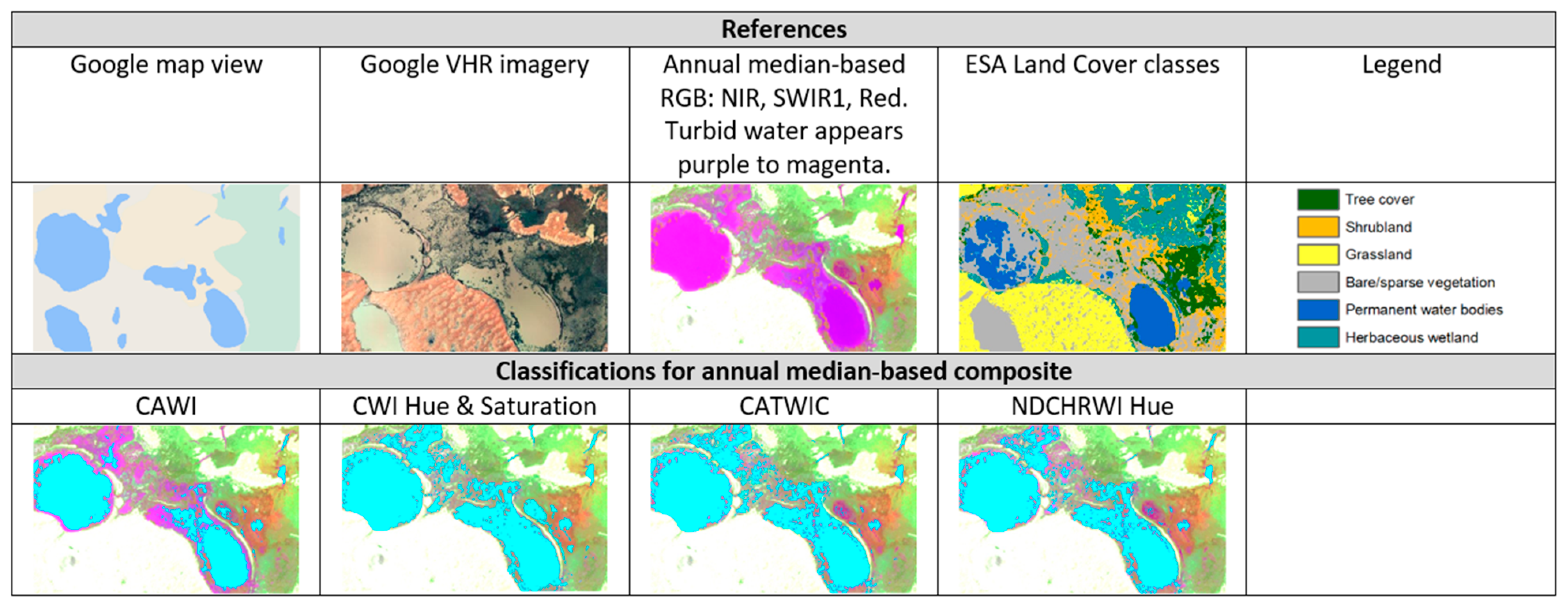
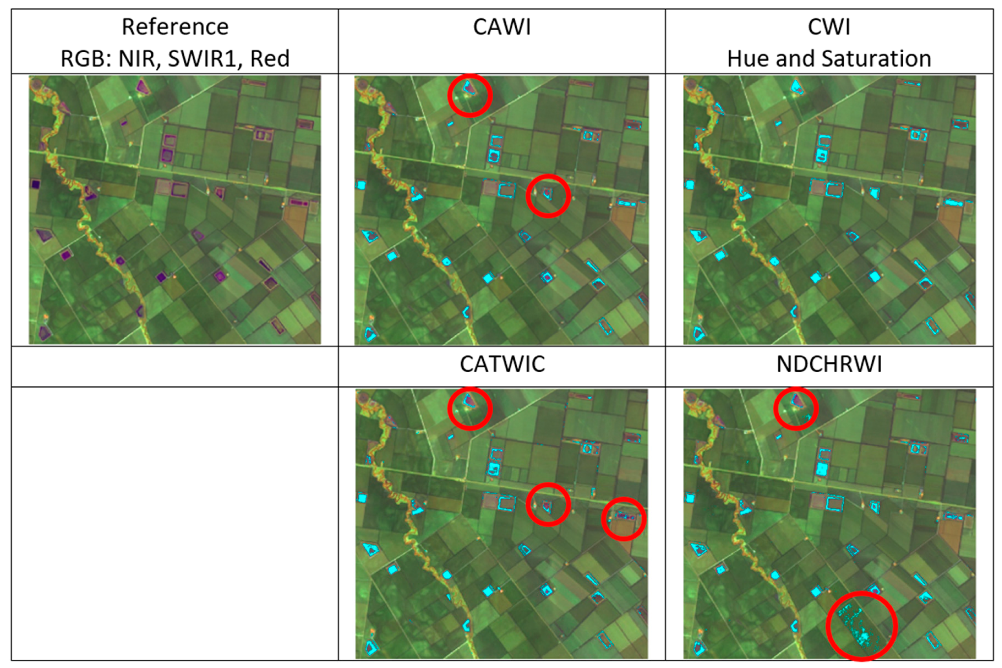


| Index | Equation | Reference |
|---|---|---|
| TCW (Tasselled Cap Wetness) | (0.1363*Blue) + (0.2802*Green) + (0.3072*Red) − (0.0807*NIR) − (0.4064*SWIR1) − (0.5602*SWIR2) | Original transformation concept by Kauth and Thomas, 1976 [11], with Sentinel-2 parameters by Nedkov, 2017 [12] |
| Normalized difference NIR/SWIR1 index (also known as NDMI or NDWI or LSWI) | (NIR − SWIR1)/(NIR + SWIR1) | Hardisky et al., 1983 [13] |
| Normalized Difference Green/SWIR1 index (also known as NDSI or MNDWI) | (Green − SWIR1)/(Green + SWIR1) | Hall et al., 1995 [14] |
| Normalized difference Green/NIR index (also known as NDWI) | (Green − NIR)/(Green + NIR) | McFeeters, 1996 [15] |
| Normalized difference Red/SWIR1 index | (Red − SWIR1)/(Red + SWIR1) | Rogers and Kearney, 2004 [16] |
| WRI | (Green + Red)/(NIR + SWIR2) | Shen and Li, 2010 [17] |
| AWEI (no shadow) | 4*(Green − SWIR1) − (0.25*NIR + 2.75*SWIR2) | Feyisa et al., 2014 [18] |
| AWEI (shadow) | Blue + (2.5*Green) − (1.5*(NIR + SWIR1)) − (0.25*SWIR2) | Feyisa et al., 2014 [18] |
| WI, 2015 | 1.7204 + (171*Green) + (3*Red) − (70*NIR) − (45*SWIR1) − (71*SWIR2) | Fisher, 2015 [19] |
| SWI | 1/(sqrt(Blue − SWIR1)) | Malahlela, 2016 [20] |
| Normalized Difference Indices | Other Indices | Indices from This Study Requiring SWIR Bands | Indices from This Study Requiring Only Visible or NIR Bands |
|---|---|---|---|
| (1) Normalized difference NIR/SWIR1 | (5) Tasselled Cap Wetness | (11) CHI | (14) CATWIC (combination of HRCWI and SR) |
| (2) Normalized difference Green/SWIR1 | (6) WRI | (12) CAWI | (15) CHRWI Hue |
| (3) Normalized difference Green/NIR | (7) AWEI (no shadow) | (13) CWI Hue, Saturation | (16) BRCHRWI Hue |
| (4) Normalized difference Red/SWIR1 | (8) AWEI (shadow) | (17) NDCHRWI Hue | |
| (9) WI, 2015 | |||
| (10) SWI |
| Criteria | Threshold Determinants and Attributes | 1 | 2 | 3 | 4 | 5 | 6 | 7 | 8 | 9 | 10 | 11 | 12 | 13 | 14 | 15 | 16 | 17 |
|---|---|---|---|---|---|---|---|---|---|---|---|---|---|---|---|---|---|---|
| Overlap of spectrally similar features | Overlaps moist evergreen forests and dark reddish tree plantations (−1) | −1,B | −1,S | 0 | 0 | 0 | 0 | 0 | 0 | 0 | −1,W | 0 | 0 | 0 | 0 | 0 | 0 | 0 |
| Overlaps intensely irrigated (bright orange) agriculture (−1) | −1,B | 0 | 0 | 0 | 0 | 0 | 0 | 0 | 0 | 0 | 0 | 0 | 0 | 0 | 0 | 0 | 0 | |
| Overlaps intensely irrigated (dark blue) agriculture (−1) | 0 | −1,B | −1,S | 0 | −1,S | 0 | −1,S | −1,S | 0 | 0 | 0 | 0 | 0 | 0 | 0 | 0 | 0 | |
| Overlaps coastal wetland features, including mangroves and sedges (−1) | −1,S | −1,W | −1,S | 0 | −1,S | 0 | −1,S | −1,S | 0 | −1,S | 0 | −1,B | 0 | 0 | 0 | 0 | −1,S | |
| Overlaps coastal sand (−1) | 0 | −1,S | −1,S | 0 | 0 | 0 | 0 | 0 | 0 | 0 | 0 | 0 | 0 | 0 | 0 | 0 | 0 | |
| Overlaps urban buildings (−1) | −1,S | −1,S | −1,S | −1,W | −1,S | −1,W | −1,S | −1,B | −1,W | −1,B | 0 | 0 | −1,B | −1,W | −1,B | −1,B | −1,S | |
| Overlaps mining areas (−1) | 0 | −1,B | −1,S | 0 | −1,S | 0 | −1,S | −1,S | 0 | 0 | 0 | 0 | 0 | 0 | 0 | 0 | 0 | |
| Overlaps coal (−1) | −1,S | −1,B | −1,B | −1,S | −1,B | −1,B | −1,B | −1,B | −1,B | −1,S | −1,S | 0 | −1,B | −1,B | −1,B | −1,B | −1,S | |
| Overlaps shadows (particularly in Winter) (−1) | −1 | −1 | −1 | −1 | −1 | −1 | −1 | −1 | −1 | −1 | −1 | −1 | −1 | −1 | −1 | −1 | −1 | |
| Overlaps snow in Winter (−1) | −1 | −1 | −1 | −1 | −1 | −1 | −1 | −1 | −1 | −1 | −1 | −1 | −1 | −1 | −1 | −1 | −1 | |
| Overlaps dry lakes or saline wetlands (−1) | 0 | −1,S | −1,S | 0 | −1,S | 0 | 0 | 0 | 0 | 0 | 0 | 0 | 0 | 0 | 0 | 0 | 0 | |
| Sensitivity | Includes most turbid water (+1) | 1 | 1 | 1 | 1 | 1 | 1 | 1 | 1 | 1 | 1 | 1 | 1 | 0 | 1 | 1 | 1 | 1 |
| Maintains narrow river detail in Summer (+1) | 0 | 1 | 0 | 0 | 1 | 0 | 1 | 0 | 0 | 1 | 1 | 1 | 1 | 1 | 1 | 1 | 0 | |
| Resolution | Requires SWIR band/s (−1) | −1 | 0 | −1 | −1 | −1 | −1 | −1 | −1 | −1 | −1 | −1 | −1 | 0 | 0 | 0 | 0 | −1 |
| Score: | −4 | −6 | −7 | −9 | −4 | −7 | −4 | −6 | −7 | −5 | −4 | −2 | −2 | −3 | −2 | −2 | −2 |
| Index | Summer | Autumn | Winter | Spring | Average | Std Dev |
|---|---|---|---|---|---|---|
| CAWI | 1.25 | 1.3 | 1.34 | 1.24 | 1.2825 | 0.04 |
| CWIHue | 0.4 | 0.4 | 0.4 | 0.4 | 0.4 | 0 |
| CWI Saturation | 0.44 | 0.44 | 0.44 | 0.44 | 0.44 | 0 |
| HRCWI | 0.2 | 0.23 | 0.2 | 0.2 | 0.2075 | 0.013 |
| SR | 0.985 | 0.985 | 0.985 | 0.985 | 0.985 | 0 |
| CHRWIHue | 0.4 | 0.4 | 0.4 | 0.4 | 0.4 | 0 |
| BRCHRWIHue | 0.37 | 0.37 | 0.37 | 0.37 | 0.37 | 0 |
| NDCHRWIHue | 0.4 | 0.4 | 0.4 | 0.4 | 0.4 | 0 |
| Reference Data | ||||||||||||
|---|---|---|---|---|---|---|---|---|---|---|---|---|
| Classes | Water | Tree Cover | Shrub Land | Grass Land | Crop Land | Built-Up | Bare/Sparse Vegetation | Herbaceous Wetland | Man-Groves | Total | User Accuracy | |
| Classified data | Water | 4501 | 2 | 0 | 2 | 0 | 0 | 0 | 0 | 1 | 4506 | 99.89% |
| Non-water | 499 | 2302 | 10 | 1935 | 684 | 31 | 28 | 14 | 9 | 5512 | 90.95% | |
| Total | 5000 | 2304 | 10 | 1937 | 684 | 31 | 28 | 14 | 10 | 10,018 | ||
| Producer accuracy | 90.02% | 99.90% | ||||||||||
| Overall accuracy: | 94.97% | |||||||||||
| Reference Data | ||||||||||||
|---|---|---|---|---|---|---|---|---|---|---|---|---|
| Classes | Water | Tree Cover | Shrub Land | Grass Land | Crop Land | Built-Up | Bare/Sparse Vegetation | Herbaceous Wetland | Man-Groves | Total | User Accuracy | |
| Classified data | Water | 4455 | 2 | 0 | 3 | 0 | 0 | 0 | 0 | 0 | 4460 | 99.89% |
| Non-water | 545 | 2302 | 10 | 1934 | 684 | 31 | 28 | 14 | 10 | 5558 | 90.19% | |
| Total | 5000 | 2304 | 10 | 1937 | 684 | 31 | 28 | 14 | 10 | 10,018 | ||
| Producer accuracy | 89.10% | 99.90% | ||||||||||
| Overall accuracy: | 94.51% | |||||||||||
| Reference Data | ||||||||||||
|---|---|---|---|---|---|---|---|---|---|---|---|---|
| Classes | Water | Tree Cover | Shrub Land | Grass Land | Crop Land | Built-Up | Bare/Sparse Vegetation | Herbaceous Wetland | Man-Groves | Total | User Accuracy | |
| Classified data | Water | 4490 | 2 | 0 | 3 | 0 | 0 | 0 | 0 | 1 | 4496 | 99.87% |
| Non-water | 510 | 2302 | 10 | 1934 | 684 | 31 | 28 | 14 | 9 | 5522 | 90.76% | |
| Total | 5000 | 2304 | 10 | 1937 | 684 | 31 | 28 | 14 | 10 | 10,018 | ||
| Producer accuracy | 89.80% | 99.88% | ||||||||||
| Overall accuracy: | 94.85% | |||||||||||
| Reference Data | ||||||||||||
|---|---|---|---|---|---|---|---|---|---|---|---|---|
| Classes | Water | Tree Cover | Shrub Land | Grass Land | Crop Land | Built-Up | Bare/Sparse Vegetation | Herbaceous Wetland | Man-Groves | Total | User Accuracy | |
| Classified data | Water | 4457 | 1 | 0 | 5 | 1 | 0 | 0 | 0 | 1 | 4465 | 99.82% |
| Non-water | 543 | 2303 | 10 | 1932 | 683 | 31 | 28 | 14 | 9 | 5553 | 90.22% | |
| Total | 5000 | 2304 | 10 | 1937 | 684 | 31 | 28 | 14 | 10 | 10,018 | ||
| Producer accuracy | 89.14% | 99.84% | ||||||||||
| Overall accuracy: | 94.50% | |||||||||||
| Histogram | ||||||||||||
| Frequency | 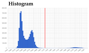 | |||||||||||
| Threshold = 1.266 | ||||||||||||
| Reference Data | ||||||||||||
|---|---|---|---|---|---|---|---|---|---|---|---|---|
| Classes | Water | Tree Cover | Shrub Land | Grass Land | Crop Land | Built-Up | Bare/Sparse Vegetation | Herbaceous Wetland | Man-Groves | Total | User Accuracy | |
| Classified data | Water | 4284 | 0 | 0 | 5 | 1 | 0 | 1 | 0 | 0 | 4291 | 99.84% |
| Non-water | 716 | 2304 | 10 | 1932 | 683 | 31 | 27 | 14 | 10 | 5727 | 87.50% | |
| Total | 5000 | 2304 | 10 | 1937 | 684 | 31 | 28 | 14 | 10 | 10,018 | ||
| Producer accuracy | 85.68% | 99.86% | ||||||||||
| Overall accuracy: | 92.78% | |||||||||||
| Histogram | ||||||||||||
| Frequency | 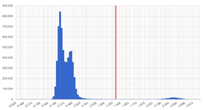 | |||||||||||
| Threshold = 1.328 | ||||||||||||
| Strata | Potential Zone Definitions | Recommended Indices | |
|---|---|---|---|
| 1 | Snow/ice covered areas | Areas mapped by MOD10A1.006 Terra Daily, Global 500 m, Snow Cover [67]. | CAWI with hill shade masking or azimuth filtering, and HRSI for a snow mask. |
| 2 | Urban areas | Areas mapped by GHSL (Global Human Settlement Layer) [66], World Settlement Footprint [68], or Tsinghua Global Artificial Impervious Areas [69], depending on local/regional performance and future currency. | CAWI, with the Saturation from CWI if further masking of extremely bright buildings is required. |
| 3 | Coastal wetland areas | An elevation- and slope-defined buffer along coastlines known to have wetland areas. | CATWIC for the greatest precision, or NDCHRWI Hue in areas such as the tropics or areas at high latitudes that are expected to have regular atmospheric haze. |
| 4 | Arid wetlands and intensely irrigated agricultural areas with highly turbid waters | Ecoregion maps such as the Resolve Ecoregions 2017 [70] for ecoregions with arid wetlands and the ESA WorldCover classes, or zonations from local ecological knowledge. | CWIHue and Saturation for fixed thresholds. |
| 5 | Mountainous areas during seasons of high hill shading | Ecoregionally specific combinations of DEM-derived elevation and slope. | SR only during Autumn and Winter, or NDCHRWI Hue during Spring and Summer with a hill shade mask. |
| 6 | Remaining areas | Areas remaining in the world from those above. | CAWI with regionally adaptive thresholding and hill shade masking (or azimuth filtering, or topographic illumination correction if <10 m DEM is available), with the HRSI as a mask for bright arid soils and salt lakes in extremely arid areas. |
| Strata | Recommended Indices | |
|---|---|---|
| 1 | Snow/ice covered areas | NDCHRWIHue with hill shade masking or azimuth filtering, and HRSI for a snow mask. |
| 2 | Urban areas | HRWI alone where no turbid water bodies are expected, or NDCHRWI Hue with the modified Saturation of Min(R,G,B)/Max(R,G,B) and HRSI as masks. |
| 3 | Coastal wetland areas | CATWIC (combination of HRCWI and SR) for the greatest precision, or the NDCHRWI Hue to mitigate atmospheric haze. |
| 4 | Intensely irrigated agricultural areas with highly turbid waters | CATWIC. |
| 5 | Mountainous areas during seasons of high hill shading | SR only between Autumn and Winter when terrain indicators cannot be remotely sensed, or NDCHRWI Hue with hill shade masking. |
| 6 | Remaining areas | NDCHRWIHue with hill shade masking or topographic illumination correction if a high resolution DEM is available, with the HRSI as a mask for bright arid soils and salt lakes in extremely arid areas. |
Disclaimer/Publisher’s Note: The statements, opinions and data contained in all publications are solely those of the individual author(s) and contributor(s) and not of MDPI and/or the editor(s). MDPI and/or the editor(s) disclaim responsibility for any injury to people or property resulting from any ideas, methods, instructions or products referred to in the content. |
© 2023 by the authors. Licensee MDPI, Basel, Switzerland. This article is an open access article distributed under the terms and conditions of the Creative Commons Attribution (CC BY) license (https://creativecommons.org/licenses/by/4.0/).
Share and Cite
Aravena, R.A.; Lyons, M.B.; Keith, D.A. Holistic Reduction to Compare and Create New Indices for Global Inter-Seasonal Monitoring: Case Study for High Resolution Surface Water Mapping. Remote Sens. 2023, 15, 2063. https://doi.org/10.3390/rs15082063
Aravena RA, Lyons MB, Keith DA. Holistic Reduction to Compare and Create New Indices for Global Inter-Seasonal Monitoring: Case Study for High Resolution Surface Water Mapping. Remote Sensing. 2023; 15(8):2063. https://doi.org/10.3390/rs15082063
Chicago/Turabian StyleAravena, Ricardo A., Mitchell B. Lyons, and David A. Keith. 2023. "Holistic Reduction to Compare and Create New Indices for Global Inter-Seasonal Monitoring: Case Study for High Resolution Surface Water Mapping" Remote Sensing 15, no. 8: 2063. https://doi.org/10.3390/rs15082063
APA StyleAravena, R. A., Lyons, M. B., & Keith, D. A. (2023). Holistic Reduction to Compare and Create New Indices for Global Inter-Seasonal Monitoring: Case Study for High Resolution Surface Water Mapping. Remote Sensing, 15(8), 2063. https://doi.org/10.3390/rs15082063


