A Registration Algorithm for Astronomical Images Based on Geometric Constraints and Homography

Abstract

The registration of astronomical images, is one of the key technologies to improve the detection accuracy of small and weak targets during astronomical image-based observation. The error of registration has a great influence on the trace association of targets. However, most of the existing methods for point-matching and image transformation lack pertinence for this actual scene. In this study, we propose a registration algorithm based on geometric constraints and homography, for astronomical images. First, the position changes in stars in an image caused by the motion of the platform where the camera had been stationed, were studied, to choose a more targeted registration model, which is based on homography transformation. Next, each image was divided into regions, and the enclosed stable stars were used for the construction of triangles, to reduce the errors from unevenly distributed points and the number of triangles. Then, the triangles in the same region of two images were matched by the geometric constraints of side lengths and a new cumulative confidence matrix. Finally, a strategy of two-stage estimation was applied, to eliminate the influence of false pairs and realize accurate registration. The proposed method was then tested on sequences of real optical images under different imaging conditions and confirmed to have outstanding performance in the dispersion rate of points, the accuracy of matching, and the error of registration, as compared to baseline methods. The mean pixel errors after registration for different sequences are all less than 0.5 when the approximate rotation angle per image is from 0.58 $\times {10}^{-2}$ to 5.89 $\times {10}^{-2}$.

1. Introduction

In recent years, the number of astronomical objects in images, including satellites and debris, has increased remarkably, making the surveillance of astronomical objects a hotspot in the field of remote sensing [1,2,3]. Many ground-based and astronomical image-based optical systems have been developed for this purpose. However, the backgrounds of the acquired astronomical images are complex, not only due to the densely distributed stars and noise, but also the complex motion of in-orbit systems, which affects the detection and tracking of targets. Image registration, which is the process of matching two images containing some of the same objects and estimating the optimal geometric transformation matrix to align the images, is a reasonable solution to the problem. The results of this registration can reduce the interference of most stars and align the trajectories of targets according to their movement rules, in order to track moving targets in the future. Among various image registration methods, feature-based image registration has become a focus of research in various fields. For astronomical images, stars are ideal and readily available feature points, as compared to commonly used features such as corner points, endpoints, edges, and so on. Therefore, there are two main methods for the registration of astronomical images: the similarity of spatial relationships and feature descriptions.

Triangle-based methods are the most common methods in this field, that are based on the similarity of spatial relationships. The traditional triangle methods focus on the mapping relationship between the stars in the detection star map and the stars in the star catalog, so that they can only be used in the known situation of the star catalog. In the reference image, every three stars within a specific range are composed into a triangle, whose angular distance is used as the side length of the triangle. If the differences between the triangles from the reference image and star catalog are within the threshold, the corresponding star points are matched. However, the biggest disadvantage of this method is its high computational demand when building and matching triangles, which limits its application in resource-constrained platforms. Many scholars have conducted significant research to solve the above challenges [4,5]. The first approach, was to reduce the number of points indexed in the catalog, with a premise of keeping valid points. The second, was to change the representation of the triangles. However, there have been few reasonable solutions to address difficulties such as low efficiency, the high consumption of memory resources, and the selection of an appropriate threshold.

Another type of triangle-based method relied only on the information of images, and the stars of two images were used to construct triangles. In order to capture translation and rotation, and the small changes in scale caused by temperature-related changes in focal length, the triangles were matched based on the triangle similarity theorem [6,7,8,9,10,11]. Groth [6], proposed a pattern-matching method to align pairs of coordinates according to two 2D lists, which had been formed from triplets of points in each list. The methods proposed by [7,8], followed a similar concept. They not only implemented, but also improved it independently, with novel strategies. On this basis, Zhou [11] proposed an improved method, based on efficient triangle similarity. He used statistical information to extract stable star points that were used to form triangles with the nearest two stable stars, and the weight matrix in triangle matching was improved by introducing a degree of similarity. The improved voting matrix was used for triangle matching. In the method proposed in [10], the authors introduced the Delaunay subdivision, which is a geometric topological structure, to further reduce the number of triangles formed by stars. The greatest defects in these methods were their extensive time requirements, high memory consumption, and their need for sophisticated voting schemes to guarantee matching accuracy. In addition, some methods used in other fields [12,13,14] even extended the triangle method to building polygons, but they encountered the same problems. At present, PixInsight [15], a relatively mature software, is a typical example of a successful application based on the triangle similarity method. The brightest 200 stars are selected, which eliminates the inefficiency caused by including all the stars in the calculation. However, there have been significant challenges when it has been applied to embedded platforms.

The methods based on feature description, have attempted to improve the registration accuracy by enhancing the feature descriptors. Generally, these methods include feature detection, feature description, and feature matching [16]. Among them, feature description has become the dominant technique. Many rotation-invariant descriptors, such as SIFT [17], SURF [18], GLOH [19], ORB [20], BRISK [21], FREAK [22], KAZE [23], and HOG [24], have been proposed and detailed in the literature [16]. The dominant orientation assignment has been the key part of these methods, to guarantee the rotation-invariant features in many applications. The estimation of the dominant orientation, requires the gradient information and the surrounding localized features, in order to calculate results.However, the gray value of stars in images decreases similarly in all directions, and the varied sizes of the local area yield inconsistent orientations, which easily produce errors in complex astronomical scenes. In addition, few of the existing methods have been devoted to the design of special descriptions for stars. Ruiz [25] applied a scale-invariant feature transform (SIFT) descriptor, to register stellar images. Zhou [16] estimated a dominant orientation from the geometrical relationships between a described star and two neighboring stable stars. The local patch size adaptively changed according to the described star size, and an adaptive sped-up robust features (SURF) descriptor was constructed.

After the matching of point pairs, the pairs are then used to solve the image transformation parameters and achieve accurate registration. The transformation in most research has been regarded as a non-rigid transformation, but translation and rotation have been the two most prominent rigid deformations [10,16]. However, the errors in registration have been significant in certain scenarios, especially when the images were significantly rotated or the point pairs were concentrated local areas. Recently, many deep-learning methods have been proposed for the estimation of these parameters. These methods can be classified into supervised [26,27] and unsupervised [28,29,30] categories. The former utilizes synthesis to generate examples with ground-truth labels for training, while the latter directly minimizes the loss of photometrics or features between images. However, these methods pose significant challenges. Firstly, the synthesized examples are unable to reflect the real scene’s parallax and dynamic objects. Secondly, the stars in the images are the key features, but their sizes are small, so the range of gray values is large, with limited texture information. When the size of the input is small and the astronomical image being processed is large, the images should be resized. In addition, there are multiple convolutional layers in the network. The two-step process further decreases the valid information of the images. Therefore, methods based on deep learning are not suitable for the registration of astronomical images.

In this work, we aimed to realize the registration of astronomical images in actual orbit. The relations between the changes in stars and the in-orbit motion of the platforms were studied, to select an accurate and effective registration model. The concept of stable stars in images was proposed in this paper. Stable stars, refers to those stars that have the highest gray values and the largest size in an image, and their appearance is usually stable across multiple images Each image was divided into regions, where the stable stars inside were selected based on statistics, to guarantee the uniformity of points for matching the whole image. Only the points in the same regions, rather than all the points, were used to construct the triangles, and therefore, the number of triangles was substantially reduced. During the matching of the triangles, the relative changes in the side length substituted for the angles, and a new cumulative confidence matrix was designed. The traditional transformation model and the proposed transformation model were coordinated, to eliminate the influence of false pairs. The former was used for the primary screening of false pairs, and the latter further estimated the parameters of the transformation on this basis, to realize an accurate registration.

As a whole, the main contributions of this paper can be summarized, as follows.

1.

We discussed in detail the changes in the stars in images caused by the in-orbit motion of the platforms and the limitations of the traditional model. An accurate and effective registration model was chosen to replace the traditional one.

2.

The triangles were characterized by their side lengths instead of their angles. Furthermore, the lengths were transformed into relative values, to reduce the difficulty of threshold settings during the matching of the triangles.

3.

A strategy with a two-stage parameter estimation, based on two different models was proposed, to realize accurate registration.

The organization of the remainder of this paper is as follows. Section 2 introduces the registration model of astronomical images in detail. In Section 3, the proposed method, along with the theoretical background, is introduced. The experimental results are presented in Section 4, the advantages and limitations of the presented method are discussed in Section 5, and the paper concludes with Section 6.

2. Registration Model for Astronomical Images

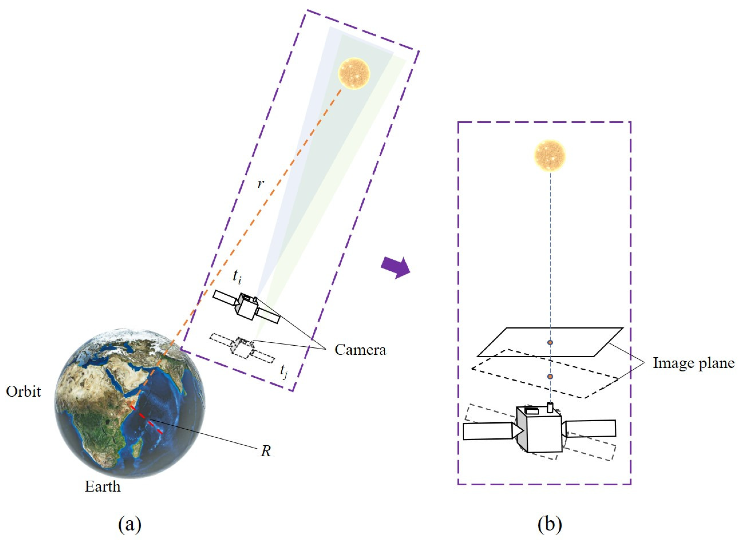
Figure 1 shows an in-orbit satellite under typical conditions and the influence of its position changes on imaging. At the times $t_i$ and $t_j$, the camera observed the same fixed star. Because the distance of the star was far greater than the orbital altitude of the satellite $r^{\prime }$, the stars in the images were infinite points, and the movement of the satellite could be ignored. Therefore, the changes in the star positions in the images were more likely caused by the change in satellite attitude at different times. The relationship between the same target in two frames of images was deduced as follows.

Let the camera’s intrinsic parameter matrix be

$$\mathbf{K}=\left[\begin{array}{ccc}{F}_x& & C_x\\ & F_y& C_y\\ & & 1\end{array}\right]$$

(1)

where $F_x$, $F_y$,$C_x$, and $C_y$ are the intrinsic parameters of the camera.

For an infinite star point, if its corresponding pixel coordinate is ${\left[x,y,1\right]}^T$ and its normalized image plane coordinate is ${\left[X,Y,1\right]}^T$, then

$$\left[\begin{array}{c}X\\ Y\\ 1\end{array}\right]={\mathbf{K}}^{-1}\left[\begin{array}{c}x\\ y\\ 1\end{array}\right]$$

(2)

where

$${\mathbf{K}}^{-1}=\left[\begin{array}{ccc}{\frac{1}{F}}_x& & -\frac{C_x}{F_x}\\ & \frac{1}{F_y}& -\frac{C_y}{F_y}\\ & & 1\end{array}\right]$$

(3)

In the coordinate system of the camera, when taking the first frame, the origin was set as the optical center, and the Z axis was set as the optical axis. Because there was only a rotational relationship between the camera attitudes, for the point whose coordinate in the first frame was ${\left[X_1,Y_1,Z_1\right]}^T$, after the attitude change matrix $\mathbf{R}$ of the camera at the imaging time of the two frames, its coordinate ${\left[X_2,Y_2,Z_2\right]}^T$ in the second frame camera coordinate system, satisfied the following:

$$\left[\begin{array}{c}\hfill X_2\hfill \\ \hfill Y_2\hfill \\ \hfill Z_2\hfill \end{array}\right]=\mathbf{R}\left[\begin{array}{c}\hfill X_1\hfill \\ \hfill Y_1\hfill \\ \hfill Z_1\hfill \end{array}\right]$$

(4)

That is, the coordinates of the point in the camera’s coordinate system of the second frame, whose coordinates on the normalized image plane of the first frame were ${\left[X,Y,1\right]}^T$, are now:

$$\left[\begin{array}{c}\hfill X^{\prime }\hfill \\ \hfill Y^{\prime }\hfill \\ \hfill Z^{\prime }\hfill \end{array}\right]=\mathbf{R}\left[\begin{array}{c}\hfill X\hfill \\ \hfill Y\hfill \\ \hfill 1\hfill \end{array}\right]$$

(5)

The optical center of the camera and the point formed a line. The coordinates of the intersection of the line and the normalized image plane was calculated by:

$$\left[\begin{array}{c}\hfill {X^{\prime }}_0\hfill \\ \hfill {Y^{\prime }}_0\hfill \\ \hfill 1\hfill \end{array}\right]=\frac{1}{Z^{\prime }}\left[\begin{array}{c}\hfill X^{\prime }\hfill \\ \hfill Y^{\prime }\hfill \\ \hfill Z^{\prime }\hfill \end{array}\right]$$

(6)

The corresponding pixel coordinates of this point in the second frame $\left(x^{\prime },y^{\prime }\right)$ were calculated as:

$$\left[\begin{array}{c}\hfill x^{\prime }\hfill \\ \hfill y^{\prime }\hfill \\ \hfill 1\hfill \end{array}\right]=\mathbf{K}\left[\begin{array}{c}\hfill {X^{\prime }}_0\hfill \\ \hfill {Y^{\prime }}_0\hfill \\ \hfill 1\hfill \end{array}\right]=\frac{1}{Z^{\prime }}\mathbf{K}\left[\begin{array}{c}\hfill X^{\prime }\hfill \\ \hfill Y^{\prime }\hfill \\ \hfill Z^{\prime }\hfill \end{array}\right]=\frac{1}{Z^{\prime }}\mathbf{K}\mathbf{R}{\mathbf{K}}^{-1}\left[\begin{array}{c}\hfill x\hfill \\ \hfill y\hfill \\ \hfill 1\hfill \end{array}\right]$$

(7)

If the attitude Euler angles of the second frame, rotating around the X, Y, and Z axes, relative to the first frame, were $\alpha$, $\beta$, and $\gamma$, respectively, and the rotation order was Z, Y, X, respectively, the relationship between it and $\mathbf{R}$ was calculated as:

$${\mathbf{R}}_x=\left[\begin{array}{ccc}1& 0& 0\\ 0& cos\alpha & -sina\\ 0& sin\alpha & cos\alpha \end{array}\right]$$

(8)

$${\mathbf{R}}_y=\left[\begin{array}{ccc}cos\beta & 0& sin\beta \\ 0& 1& 0\\ -sin\beta & 0& cos\beta \end{array}\right]$$

(9)

$${\mathbf{R}}_z=\left[\begin{array}{ccc}cos\gamma & -sin\gamma & 0\\ sin\gamma & cos\gamma & 0\\ 0& 0& 1\end{array}\right]$$

(10)

$$\mathbf{R}={\mathbf{R}}_z{\mathbf{R}}_y{\mathbf{R}}_x=\left[\begin{array}{ccc}{r}_1& r_2& r_3\\ r_4& r_5& r_6\\ r_7& r_8& r_9\end{array}\right]$$

(11)

where

$$\begin{array}{l}{r}_7=sin\alpha sin\gamma -cos\alpha cos\gamma sin\beta \\ r_8=cos\gamma sin\alpha cos\alpha sin\beta sin\gamma \\ r_9=cos\alpha cos\beta \end{array}$$

(12)

The above deductions were regarded as the process of homography transformation. The homography matrix can be written as:

$$\mathbf{H}=\frac{1}{Z^{\prime }}\mathbf{KR}{\mathbf{K}}^{-1}=\left[\begin{array}{ccc}{h}_1& h_2& h_3\\ h_4& h_5& h_6\\ h_7& h_8& h_9\end{array}\right]$$

(13)

If the relationship between two images could be approximated as the translational and rotational relationship of the image, that is, the affine transformation that was commonly used in this field, it was equivalent to the existence of ${\mathbf{R}}_0$ and ${\mathbf{T}}_0$, satisfying:

$$\frac{1}{Z^{\prime }}\mathbf{KR}{\mathbf{K}}^{-\mathbf{1}}\approx \left[\begin{array}{cc}{\mathbf{R}}_0& {\mathbf{T}}_0\\ \mathbf{0}& 1\end{array}\right]$$

(14)

The third row of $\mathbf{KR}{\mathbf{K}}^{-\mathbf{1}}$ was calculated as:

$$\left[\begin{array}{ccc}\frac{r_7}{F_x}& \frac{r_8}{F_y}& r_9\end{array}\right]$$

(15)

Then, the above problem could be simplified to at least meet the following condition:

$$\left[\begin{array}{ccc}\frac{r_7}{F_x}& \frac{r_8}{F_y}& r_9\end{array}\right]\approx \left[\begin{array}{ccc}0& 0& Z^{\prime }\end{array}\right]$$

(16)

If, and only if, $\alpha$ and $\beta$ were close to 0, and $Z^{\prime }$ was close to 1, ${\mathbf{R}}_0$ and ${\mathbf{T}}_0$ could be solved. However, when the satellite operated in an orbit at an altitude of 200–2000 km from the ground, the time for it to orbit the earth was 90–120 min, so that the operating angular speed was 3–4 arcmin per second. In this scenario, the attitude of the satellite changed rapidly, and the translation and rotation of the image could not reflect the actual changes in the image. Therefore, the image registration model based on homography transformation was applied in this paper.

3. The Matching Method for Stars

Because the locations of fixed stars are salient features in images, fixed stars in two images for matching were selected to calculate the transformation matrix.

3.1. Triangle Construction

For the selected star points in the reference map and the target map, every three stars were combined as triangles, to form sets $T_{ref}$ and $T_{src}$, respectively. A total of k star points could generate up to $C_k^3$ triangles. Therefore, the number of constructed triangles was positively correlated with the number of stars. Because of the large number of stars detected, the computational demand was significant.arszalek [4] used the brighter stars in the star points to construct triangles. This method had two problems, however: (1) the threshold of selecting bright stars was uncertain. The selection threshold directly affected the number of star points involved in the construction of the triangles. If the threshold was too low, the number of stars involved in the calculation was too large, making it difficult to achieve efficiency. When the threshold was high, the points could be insufficient. (2) Tuytelarrs et al. [31,32] proposed that the feature points should be evenly distributed across the whole image, in order to estimate the transformation matrix more accurately. The study in [4] could not ensure that the selected bright stars were evenly distributed across the whole image.

In order to resolve the above problems, we searched for limited stable stars in an image. However, there could be stray light, thermal noise, and other effects in the images, and some pixels and even regions could also have local highlights. It was difficult to achieve a global star search only through a single fixed threshold. Therefore, the image was divided into $N\times M$ regions. For a single region, the gray values of the contained pixels were counted, to realize the dynamic setting of the threshold, and the image was binarized, as follows:

$$\begin{array}{c}{I}_{bw}\left(x,y\right)=\left\{\begin{array}{cc}0& I\left(x,y\right)<T_g\\ 1& I\left(x,y\right)\ge T_g\end{array}\right.\\ T_g=c_{sort}(\alpha \times n_p)\end{array}$$

(17)

where $T_g$ is the threshold of gray value. The variable $c_{sort}$ is the sequence formed by arranging the gray values of all $n_p$ pixels in the local area from small to large, and $\alpha$ is the scale coefficient. If the gray value of a pixel was higher than the $\alpha$% of the points in the region, the pixel was set to 1 in the binary image $I_{bw}$. The connected regions in $I_{bw}$ were sorted by area, and the $N_{*}$ largest connected regions were selected as local stable stars. In this way, we significantly reduced the influence of strong isolated interference, such as thermal noise. The weighted centroids of stable stars were calculated as centers. For the connected domain of $n_l$ pixels, the calculation was as follows:

$$\begin{array}{c}\hfill x_c=\frac{{\displaystyle \sum _{i=1}^{n_l}}I\left(x_i,y_i\right)x_i}{{\displaystyle \sum _{i=1}^{n_l}}I\left(x_i,y_i\right)}\hfill \\ \hfill y_c=\frac{{\displaystyle \sum _{i=1}^{n_l}}I\left(x_i,y_i\right)y_i}{{\displaystyle \sum _{i=1}^{n_l}}I\left(x_i,y_i\right)}\hfill \end{array}$$

(18)

where $\left(x_c,y_c\right)$ is the center of a star, and $I\left(x_i,y_i\right)$ is the gray value of point $\left(x_i,y_i\right)$. These stable stars were used to generate $C_{N_{*}}^3$ triangles.

The camera was usually attached to a satellite. If the attitudes of both the satellite and camera were stable, the movement distance of the stable star between frames was usually minimal. The registration of the corresponding star points was also carried out in each region for better efficiency. The set of all the triangles $\mathbb{N}$, in a region, was formed as follows:

$$\mathbb{N}=\left\{\left.{\mathsf{\Delta }}_{i,j,k}\right|\forall i,j,k\in \left\{12\cdots ,N_{*}\right\}i<j<k\le N_{*}\right\}$$

(19)

where ${\mathsf{\Delta }}_{i,j,k}$ is the triangle with the vertices of three star points $i,j,k$.

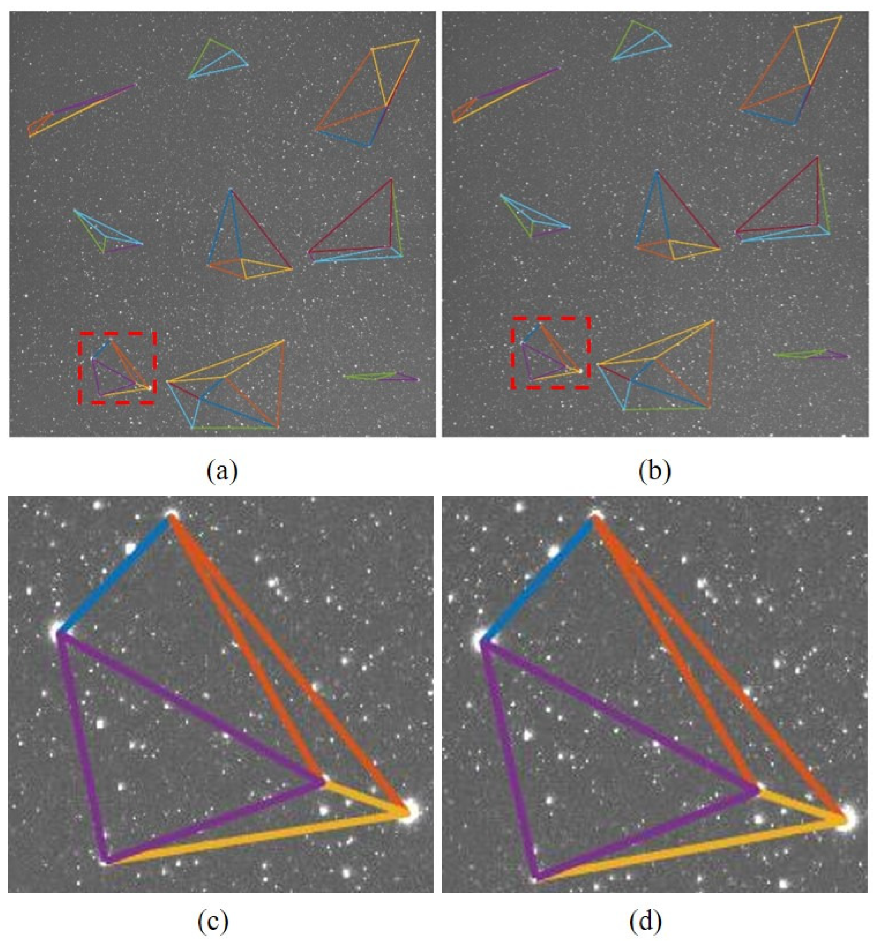
Figure 2 shows an illustration of the triangle construction. Two images significantly affected by stray light were divided into 3 × 3 regions, and then six stable stars were chosen. For a better visual effect, only the triangles satisfying Delaunay remained.

3.2. Triangle Matching

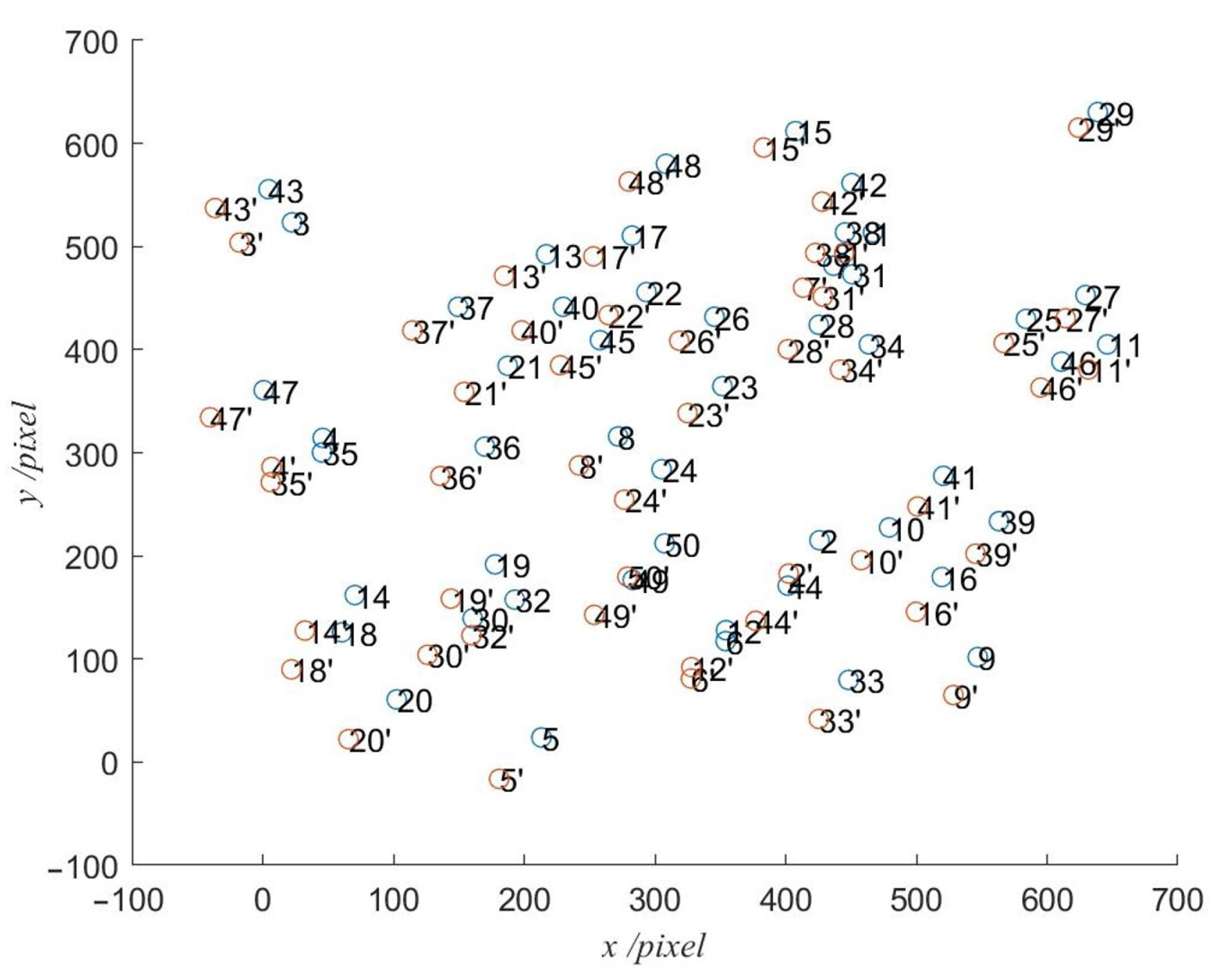
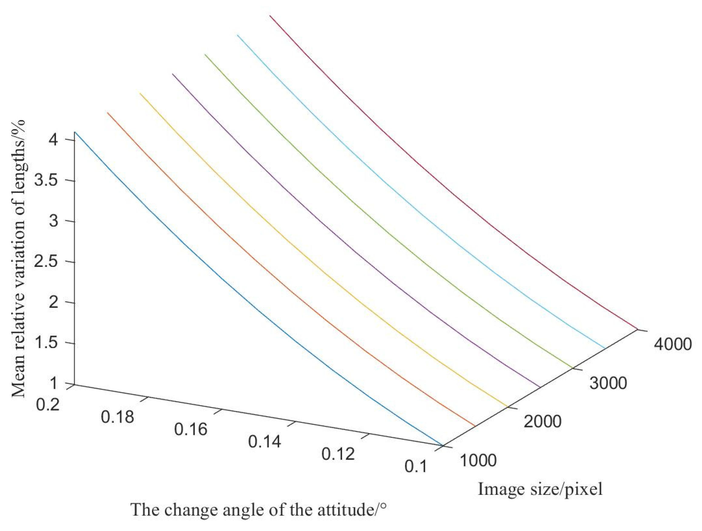
Due to the movement of the observational platform, the gray values, positions, and sizes of star points in two frames could change. To identify the stable features of the triangles before and after movement, images of different sizes, from 1000 to 4000 pixels, were divided into $3\times 3$ regions, and 50 points were randomly generated inside, to simulate the stable stars. The attitude of the camera was changed from $0.1^{\circ }$ to $0.2^{\circ }$ around the x and y axes, as shown in Figure 3. The relative variations in lengths of the segment lines formed by the points were recorded. The statistical results showed that the relative variations in the lengths between the star points in two frames, were smaller than 4% within the slight movement caused by the change in attitude, as shown in Figure 4. This indicated that the side lengths of the triangles composed of stars were stable. In this paper, a registration method based on the triangular length constraint was proposed, to match the corresponding star points.

To match triangles, we used the feature information of the triangles. The features of triangles included three sides and three angles. In order to facilitate our calculations, this study used the length of the three sides to build a clue matrix. The clue matrix $\mathbf{Z}$, was divided into $C_{N_{*}}^3$ rows, and each row was used to store the lengths of three sides of a triangle and the numbers of three vertices. The specific format was as follows:

$$\mathbf{Z}=\left[\begin{array}{cccccc}{l}_{12}& l_{13}& l_{23}& 1& 2& 3\\ l_{12}& l_{14}& l_{24}& 1& 2& 4\\ ⋮& ⋮& ⋮& ⋮& ⋮& ⋮\\ l_{N_{*}-2,N_{*}-1}& l_{N_{*}-2,N_{*}}& l_{N_{*}-1,N_{*}}& N_{*}-2& N_{*}-1& N_{*}\end{array}\right]$$

(20)

where $l_{ij}$ is the distance between the ith and jth star points.

After the clue matrices of the corresponding regions in two images were constructed, and recorded as Z and $Z^{\prime }$, they were used for the registration of corresponding star points. The registration was primarily divided into two steps. The first step involved matching the triangles, and the second step involved matching the points. The judgment basis of the triangle matching, was that the corresponding side lengths of the two triangles were almost equal. Because the side lengths of each triangle were arranged in a different order in the two clue matrices, it was necessary to adjust the side lengths’ order first. The matching of points was based on the success of the triangle matching. The three sides of the two triangles corresponded to each other individually. The matching of points was carried out according to the principle that, the vertices of the two corresponding sides were corresponding star points. The steps of the registration were as follows:

(1)

The first three columns of $\mathbf{Z}$ and ${\mathbf{Z}}^{\prime }$ were extracted, and each row was rearranged from small to large to form matrices $\mathbf{L}$ and ${\mathbf{L}}^{\prime }$, respectively.

(2)

The triangles ${\mathsf{\Delta }}_{1,2,3}$ in the first row of $\mathbf{L}$, were extracted for pairing. The relative differences between the three side lengths of ${\mathsf{\Delta }}_{1,2,3}$ and the side lengths of all the triangles in ${\mathbf{L}}^{\prime }$ were calculated, and the relative difference matrix $\mathbf{D}$ was constructed as follows:

$$\mathbf{D}=\left[\begin{array}{ccc}\frac{l_{1^{\prime }{2}^{\prime }}-l_{12}}{l_{12}}& \frac{l_{1^{\prime }{3}^{\prime }}-l_{13}}{l_{13}}& \frac{l_{2^{\prime }{3}^{\prime }}-l_{23}}{l_{23}}\\ \frac{l_{1^{\prime }{2}^{\prime }}-l_{12}}{l_{12}}& \frac{l_{1^{\prime }{4}^{\prime }}-l_{13}}{l_{13}}& \frac{l_{2^{\prime }{4}^{\prime }}-l_{23}}{l_{23}}\\ ⋮& ⋮& ⋮\\ \frac{l_{4^{\prime }{5}^{\prime }}-l_{45}}{l_{12}}& \frac{l_{4^{\prime }{6}^{\prime }}-l_{46}}{l_{13}}& \frac{l_{5^{\prime }{6}^{\prime }}-l_{56}}{l_{23}}\end{array}\right]$$

(21)

(3)

The smallest value in $\mathbf{D}$ was regarded as the lowest sum value of the differences of each side $D_{single}$ and the differences of the sum of the three sides $D_{all}$, which was defined as follows:

$$\begin{array}{cc}\hfill min\left\{\mathbf{D}\right\}& \hfill =D_{single}\left(1\right)+D_{single}\left(2\right)+D_{single}\left(3\right)+D_{all}\hfill \\ \hfill \end{array}$$

(22)

where

$$\begin{array}{c}{D}_{single}\left(1\right)=\frac{\left|l_{i^{\prime }{j}^{\prime }}-l_{12}\right|}{l_{12}},D_{single}\left(2\right)=\frac{\left|l_{i^{\prime }{k}^{\prime }}-l_{13}\right|}{l_{13}},D_{single}\left(3\right)=\frac{\left|l_{j^{\prime }{k}^{\prime }}-l_{23}\right|}{l_{23}}\\ D_{all}\left(1\right)=\left|\frac{l_{i^{\prime }{j}^{\prime }}-l_{12}}{l_{12}}+\frac{l_{i^{\prime }{k}^{\prime }}-l_{13}}{l_{13}}+\frac{l_{j^{\prime }{k}^{\prime }}-l_{23}}{l_{23}}\right|\\ \end{array}$$

(23)

where $i^{\prime },j^{\prime },k^{\prime }$ are the number of stars in ${\mathbf{Z}}^{\prime }$.

(4)

If the relative changes in the distances met the following standard: the difference of each side was smaller than $10\%$, and the sum of the difference was smaller than $5\%$, the pair was judged a success, that is:

$$\begin{array}{c}\left\{\begin{array}{c}\hfill D_{single}\left(i\right)\le 10\%\bigcap D_{all}\le 5\%\Rightarrow {\mathsf{\Delta }}_{i^{\prime },j^{\prime },k^{\prime }}\cong {\mathsf{\Delta }}_{1,2.3}\hfill \\ \hfill D_{single}\left(i\right)>10\%\bigcup D_{all}>5\%\Rightarrow \left[\right]\cong {\mathsf{\Delta }}_{1,2.3}\hfill \end{array}\right.\\ i=1,2,3\end{array}$$

(24)

where ≅ means the success of pairing and $\left[\right]$ means no matching reference triangle.

(5)

If the matching of ${\mathsf{\Delta }}_{i^{\prime },j^{\prime },k^{\prime }}$, and ${\mathsf{\Delta }}_{1,2.3}$ was successful, the corresponding points would be matched next. The variables $l_{i^{\prime }{j}^{\prime }}$, $l_{i^{\prime }{k}^{\prime }}$, $l_{j^{\prime }{k}^{\prime }}$ and $l_{12}$, $l_{13}$, $l_{23}$ had one-to-one correspondence. The intersection of $l_{i^{\prime }{j}^{\prime }}$ and $l_{i^{\prime }{k}^{\prime }}$ was $i^{\prime }$, and the intersection of $l_{12}$ and $l_{13}$ was 1, so $i^{\prime }$ and 1 were corresponding points. Similarly, $j^{\prime }$ and 2, as well as $k^{\prime }$ and 3, were also corresponding points. Considering that there could be mismatched triangle pairs, a weight matrix of $N_{*}\times N_{*}$ was constructed. Each row in the weight matrix represented a star point in the previous image, and each column represented a star point in the current image. Each intersection represented a pair of star points, and its value represented the cumulative confidence of the matching. Single confidence $v^{\prime }$, was defined as follows:

$$v^{\prime }\left(m,n\right)=2-D_{m,n}$$

(25)

where m and n are the two points in single matching, and $D_{m,n}$ is the sum of the absolute value of the relative differences between the two sides, in triangles corresponding to the matched points.

(6)

The operations of (2)–(5) were repeated until all triangles in L had been matched. The cumulative confidence v, was the result after the registration of all triangles:

$$v\left(m,n\right)=\sum v^{\prime }\left(m,n\right)$$

(26)

If $v\left(m,n\right)$ is the maximum value of the mth row and the nth column and $v\left(m,n\right)>5$, that is, the matching of two points had been successful, the star number of the corresponding point pair in the ith region would be saved in pair matrix $P_i$.

(7)

The same processing was carried out for each region. The information of the matched points in $P_i$ was summarized in $P_{total}$.

3.3. Parameter Estimation

The points in $P_{total}$ were used to calculate the homography matrix between two frames. The pixel coordinate of a corresponding point in the second frame $\left(x^{\prime },y^{\prime }\right)$ could be calculated as follows:

$$\left\{\begin{array}{c}\hfill x^{\prime }=\frac{h_{1}x+h_{2}y+h_3}{h_{7}x+h_{8}y+h_9}\hfill \\ \hfill y^{\prime }=\frac{h_{4}x+h_{5}y+h_6}{h_{7}x+h_{8}y+h_9}\hfill \end{array}\right.$$

(27)

Considering the reasons for scaling, there were only eight unknowns, rather than nine, when solving $\mathbf{H}$. Once a certain value was assigned to any non-zero element in the matrix, other elements would also acquire a certain value, according to the proportion. Usually, the matrix used was obtained by setting the value of $h_9$ to 1, which was recorded as follows:

$${\mathbf{H}}_{\mathbf{0}}=\mathbf{H}$$

(28)

This ensured the values of elements $h_3$ and $h_6$ were equal to $x^{\prime }$ and $y^{\prime }$, respectively, when x and y were each equal to 0.

From the previous derivation, for each pair of points on two planes, two equations based on x and y could be established simultaneously:

$$\left\{\begin{array}{c}\hfill h_{1}x+h_{2}y+h_3-h_7{x}^{\prime }x-h_8{x}^{\prime }y-h_9{x}^{\prime }=0\hfill \\ \hfill h_{4}x+h_{5}y+h_6-h_7{y}^{\prime }x-h_8{y}^{\prime }y-h_9{y}^{\prime }=0\hfill \end{array}\right.$$

(29)

That is

$$\begin{array}{c}\left\{\begin{array}{c}\hfill \mathbf{X}=\left(\begin{array}{ccccccccc}x& y& 1& 0& 0& 0& -x^{\prime }x& -x^{\prime }y& -x^{\prime }\end{array}\right)\hfill \\ \hfill \mathbf{Y}=\left(\begin{array}{ccccccccc}0& 0& 0& x& y& 1& -y^{\prime }x& -y^{\prime }y& -y^{\prime }\end{array}\right)\hfill \end{array}\right.\\ \mathbf{h}={\left(\begin{array}{ccccccccc}{h}_1& h_2& h_3& h_4& h_5& h_6& h_7& h_8& h_9\end{array}\right)}^T\end{array}$$

(30)

The solution of the matrix $\mathbf{H}$ required eight constraints, so more than four pairs of points needed to be provided to achieve this. For $n_{total}$ pairs of points, we could obtain the following:

$$\mathbf{Ah}=0$$

(31)

where

$$\begin{array}{c}\mathbf{A}={\left[\begin{array}{ccccccc}{\mathbf{X}}_1& {\mathbf{Y}}_1& {\mathbf{X}}_2& {\mathbf{Y}}_2& \cdots & {\mathbf{X}}_{n_{total}}& {\mathbf{Y}}_{n_{total}}\end{array}\right]}^T\\ n_{total}\ge 4\end{array}$$

(32)

The solution for this equation was then transformed to the following:

$$\begin{array}{c}min\left|\right|\mathbf{Ah}\left|\right|\\ \mathrm{s}.\mathrm{t}.\left|\right|\mathbf{h}\left|\right|=1\end{array}$$

(33)

and

$$min\left|\right|\mathbf{Ah}\left|\right|=min\left|\right|UDVT\mathbf{h}\left|\right|=min\left|\right|DVT\mathbf{h}\left|\right|$$

(34)

where D is a diagonal matrix, and the diagonal elements were arranged in descending order. The optimal solution was obtained when $x={\left(0,0,...,1\right)}^T$, and the column vector corresponding to the minimum singular value of V was the solution of parameters.

Since the number of pairs was obviously more than the requirement, there could be some mismatched pairs. These mismatched pairs resulted in a large calculation error of $\mathbf{H}$, though even their projection errors were not always the largest. In contrast, when using translation and rotation to approximate homography transformation, the mismatched point pairs usually pointed to the largest projection errors. Therefore, a two-stage iteration was calculated as follows:

(1)

$P_{total}$ and Equation (13) were used to calculate ${\mathbf{R}}_{\mathbf{0}}$ and ${\mathbf{T}}_{\mathbf{0}}$, by the least squares method.

(2)

The projection calculations were carried out for each point using the calculated ${\mathbf{R}}_{\mathbf{0}}$ and ${\mathbf{T}}_{\mathbf{0}}$, and the projection error of a single point was

$${\epsilon }_i=\sqrt{{\left(\tilde{x}-x^{\prime }\right)}^2+{\left(\tilde{y}-y^{\prime }\right)}^2}$$

(35)

where ${\epsilon }_i$ is the projection error of the ith point, the point $\left(\tilde{x},\tilde{y}\right)$ is the result of the projection calculation of point $\left(x,y\right)$ in the previous frame, and $\left(x^{\prime },y^{\prime }\right)$ is the pairing point of the point $\left(x,y\right)$ in the current frame.

(3)

If the average error was higher than the error threshold $T_{\epsilon }$, that is

$$mean\left({\epsilon }_i\right)>T_{\epsilon }$$

(36)

then the point pairs with the largest errors (greater than 95% of ${\epsilon }_i$) were eliminated, and the calculation was restarted from 1.

If

$$mean\left({\epsilon }_i\right)\le T_{\epsilon }$$

(37)

then all the remaining pairs were correct pairs, and the iteration stopped. The correct pairs would be used for the calculation of $\mathbf{H}$.

4. Experimental Results and Discussion

The proposed method was applied to realize the registration of real astronomical images. All experiments were implemented by using the MATLAB R2020a software, on a PC with 16 GB memory and a 1.9 GHz Intel i7 dual processor. During the experiments, the same empirical parameters were used, as follows:

(1)

The image was divided into $\left(N=\right)3\times \left(M=\right)$3 regions.

(2)

The points with gray values higher than $\alpha =99.95\%$ of the points in the region were set to 1.

(3)

A total of $N_{*}=8$ fixed stars in each region were chosen to generate triangles.

(4)

The error threshold was $T_{\epsilon }=0.5$.

4.1. Experimental Settings

(1)

Dataset

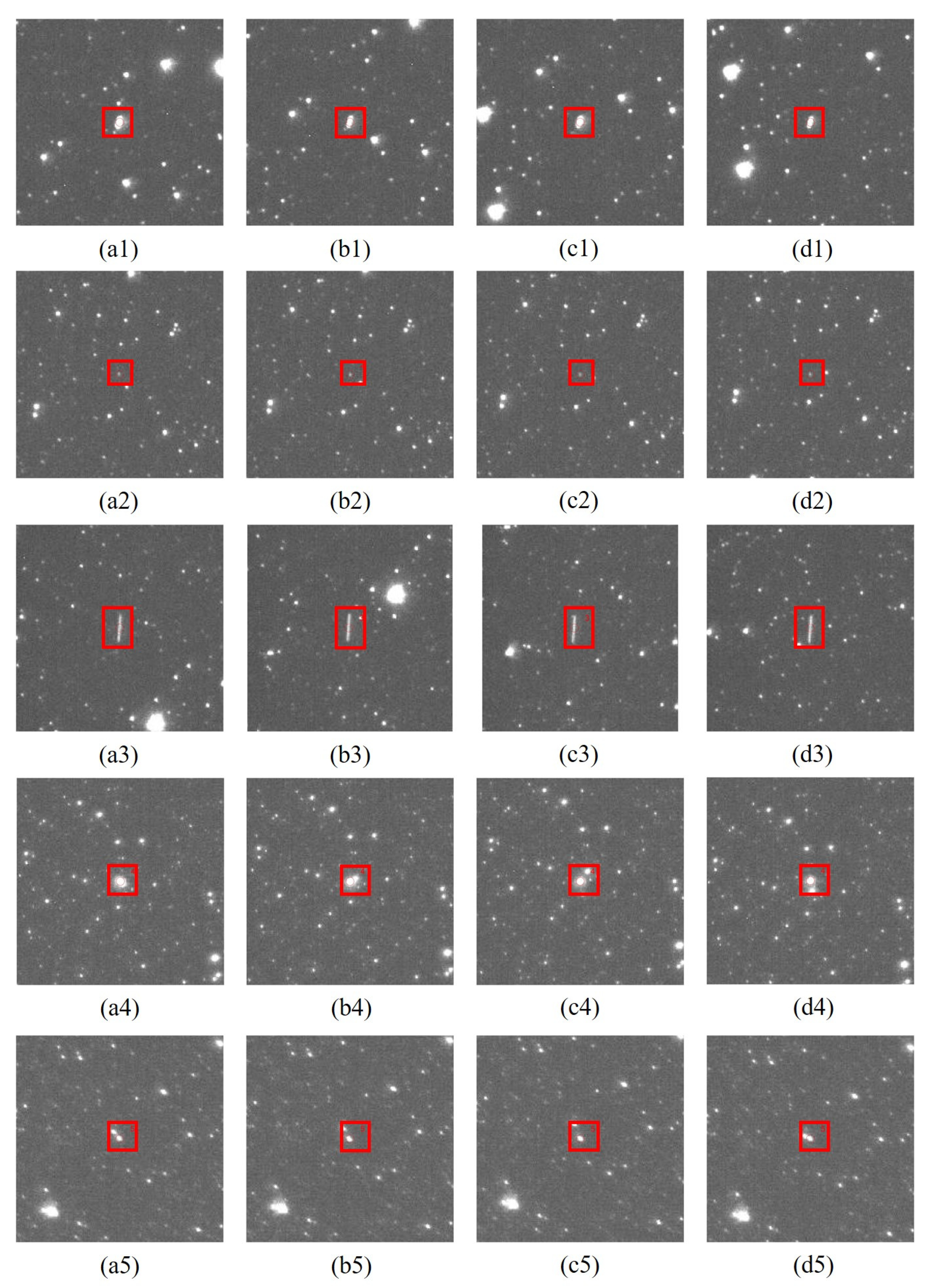
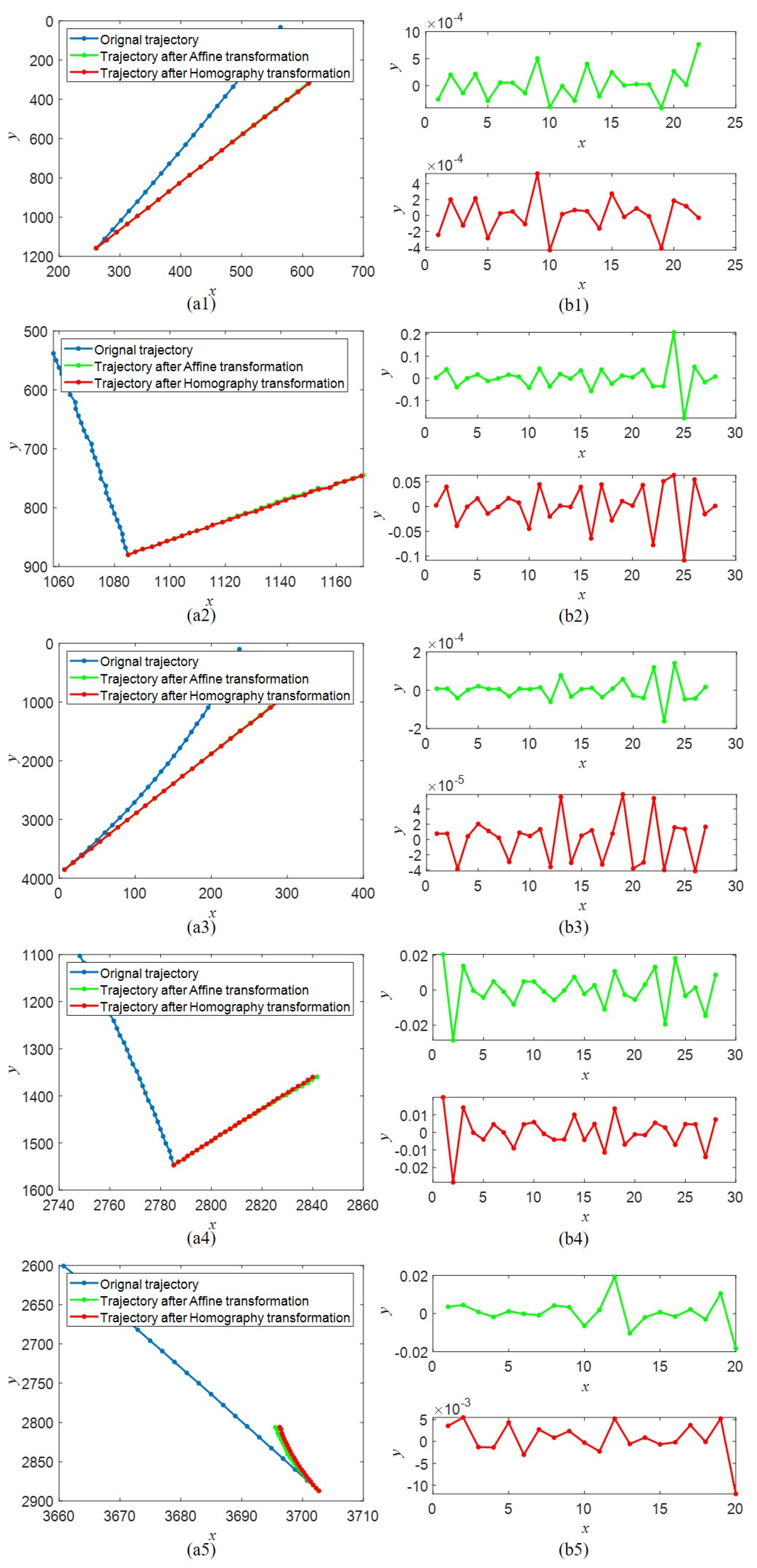
Because there was no relevant public dataset, the experiments were carried out on six different sequences, whose data were 16-bit, to verify the performance of the proposed method in this paper. The sequences were acquired by three space-based telescopes and two ground-based telescopes, with different camera parameters and under different representative imaging conditions, denoted as Seq.1–Seq.6, and the details are listed in

Table 1. Information of telescopes in sequences.

Seq.	Platform	Number of Images	Image Size	Field Angle (${}^{\circ }$)	Approximate Rotation Angle per Image (${}^{\circ }$)
1	Space-based	30	4096 × 4096	20 × 20	5.89 $\times {10}^{-2}$
2	Ground-based	13	4096 × 4096	13.1 × 13.1	5.35 $\times {10}^{-2}$
3	Space-based	20	4096 × 4096	15 × 15	0.22 $\times {10}^{-2}$
4	Space-based	20	4096 × 4096	15 × 15	0.68 $\times {10}^{-2}$
5	Ground-based	20	1024 × 1024	1.07 × 1.07	0.29 $\times {10}^{-2}$
6	Ground-based	10	1024 × 1024	1.07 × 1.07	0.58 $\times {10}^{-2}$

and

Table 2. Information of images in sequences.

Seq.	Approximate Movement per Image	Gray Value Information
		Maximum	Mean	Minimum	Standard Deviation
1	7.46	65,535.00	105.05	50.00	148.91
2	11.14	37,790.00	142.91	48.00	26.28
3	8.29	4071.00	778.63	0.00	66.63
4	25.04	4074.00	1097.30	0.00	88.49
5	8.20	32,529.00	5486.20	0.00	237.58
6	20.20	7968.00	593.43	457.00	40.79

. One typical image in each sequence was processed using gray stretching for illustration, as shown in Figure 5. Among them, Seq.2 and Seq.5 were significantly influenced by stray light, which is one kind of large-area interference. Stray light may affect the selection of stable stars, especially when its gray value is close to those of stars.he stray light was distributed unevenly in an image, and moved and changed slowly across sequences. The stray light in Seq.2 was diffused from the left–bottom side to the right–top side of the images, while in Seq.5, it was concentrated in the middle area. The gray value of stray light in the region of the diffusion source was strong, and gradually decreased with the diffusion. There were rows or columns of dark pixels in Seq.3 and Seq.4. The shapes of stars in Seq.1–Seq.3 were point-like, while those in Seq.4–Seq.6 were streak-like. Furthermore, all the sequences had the issue of common noise interference, such as thermal noise, due to real-world conditions. All five visible targets in the sequences were chosen to compare the changes in trajectories before and after registration, as shown in Figure 6.

(2)

Baselines

The representative methods proposed in [10,16,18,20] were selected, and combined as baselines in this paper. Among them, establishing a global threshold for image binarization has been a common method for the selection of stable stars. SURF and ORB have been the most widely used and classic descriptors for the matching of corresponding points. Using the triangle relations between stars has been another commonly used method in this field. Zhou [16] constructed the triangle relations between stars with a global threshold, and embedded the relations into SURF. Yang [10] used the Delaunay subdivision to describe the triangle relations between stable stars.

(3)

Evaluation metrics

A dispersion rate ($DR$) of the initial selected stable stars for triangle construction, directly affected the calculation of $\mathbf{H}$. For a reasonable quantification of this index, an image was divided into grids ($n\times n$), and $DR$ was defined as follows:

$$DR=\sqrt{\frac{{{\displaystyle \sum _{i=1}^{n\times n}}\left(c_i-\overline{c}\right)}^2}{n-1}}$$

(38)

where $c_i$ is the number of points in the ith grid.

After selecting the stable stars, their corresponding pairs of points were then matched. The accuracy of matching was defined as follows:

$$Accurac{y}_m=\frac{N_{cp}}{N_p}$$

(39)

where $N_{cp}$ is the number of correct pairs and $N_p$ is the number of pairs.

The corresponding pairs were used to estimate the parameters of different transformation methods. The points belonging to the pairs in one image were projected onto another image. The pixel error, $Erro{r}_{ij}$, of the projection points from the jth image to the ith image, and the original points in the ith image, were defined as follows:

$$Erro{r}_{ij}=\frac{{\displaystyle \sum _{i=1}^{N_p}}\sqrt{{(x_i-x_{ji})}^2+{(y_i-y_{ji})}^2}}{N_p}$$

(40)

where $\left(x_i,y_i\right)$ and $\left(x_{ji},y_{ji}\right)$ are the image coordinates of the original points and projection points, respectively.

The targets was also projected from the images onto the reference image, and formed the corresponding trajectories. Non-linear least squares fitting [33] was utilized for these trajectories. In addition to the typical statistical indices, such as SSE, R-squared, and RMSE, curvature was also used, to determine the degree of smoothness of the fitting results. The curvature K, was defined as follows:

$$K=\frac{|\dot{x}\ddot{y}-\ddot{x}\dot{y}|}{|{\dot{x}}^2+{\dot{y}}^2{|}^{\frac{3}{2}}}$$

(41)

4.2. Comparative Analysis of the Corresponding Point-Matching

In this section, the proposed method is realized in stages and compared to baselines. In the experiment, the first image was regarded as the reference image. The subsequent images were registered to the reference image, to simulate different deviations caused by different movement speeds of the platform and the time intervals for imaging. During stable star selection, each baseline was used to select 100 points in an image, in order to ensure the number of valid stable stars and match the number of stable stars determined by the proposed method. Each image was divided into a $4\times 4$ grid, and the results of the average dispersion rate are shown in

Table 3. Comparison of dispersion rates of selected stable stars among the proposed method and baselines.

Seq.	Number of Points/Average Dispersion Rate
	Global Threshold	SURF	ORB	Ours
1	100/2.54	100/2.91	100/4.99	72/1.63
2	100/4.29	100/5.03	100/6.42	72/1.59
3	100/3.31	100/5.83	100/4.24	72/1.68
4	100/4.32	100/5.70	100/4.57	72/1.44
5	100/2.29	100/4.49	100/8.61	72/1.30
6	100/2.51	100/5.20	100/8.39	72/1.85

. The dispersion rate of the points chosen by the global threshold methods, SURF and ORB, had an excellent range variance. The distributions of stars found by the proposed method in astronomical images were reasonably balanced, which benefited their registration.

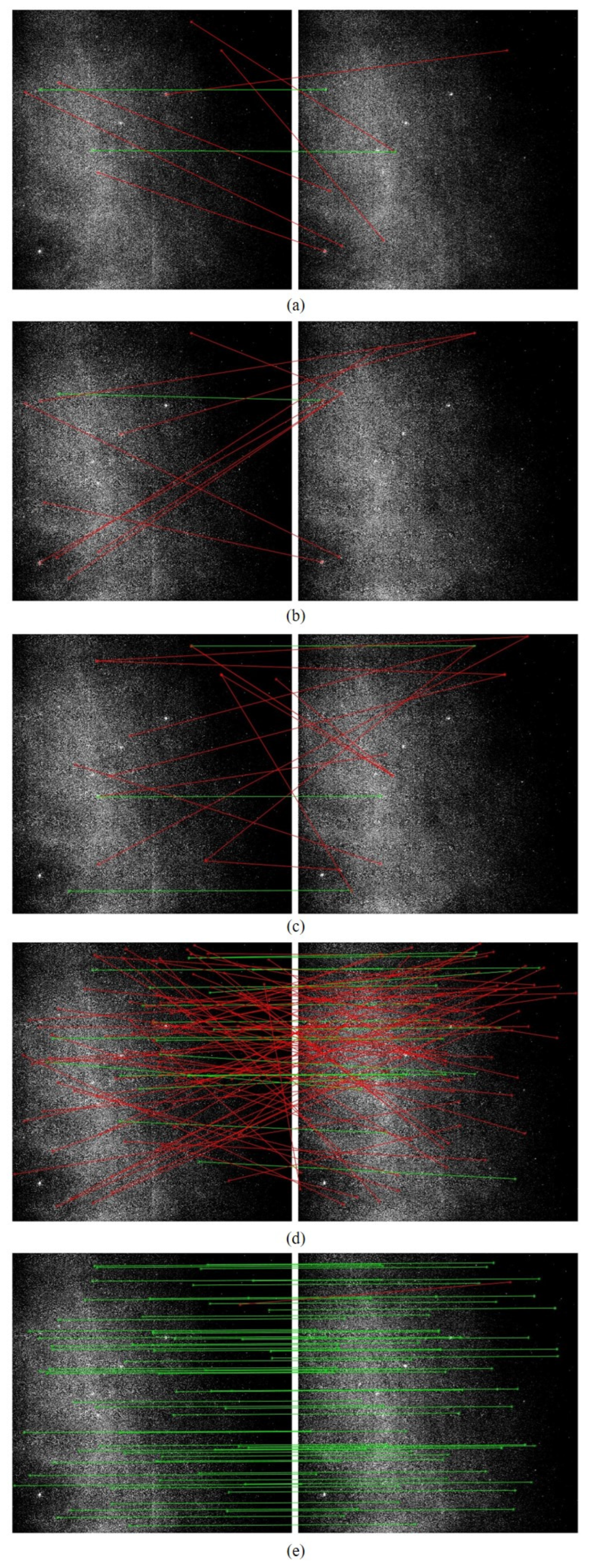
The selected stable stars in two images contained corresponding points, which were further confirmed by the baselines and the proposed method. The number of point pairs and the accuracy had a significant impact on the subsequent parameter estimations of the transformation matrix. Figure 7 and

Table 4. Comparison of corresponding point-matching among the proposed method and baselines.

Seq.	${\mathit{N}}_{\mathit{p}}$/${\mathit{N}}_{\mathbf{cp}}$/${\mathbf{Accuracy}}_{\mathit{m}}$
	SURF	Global Threshold + Improved SURF	ORB	Global Threshold + Delaunay	Ours
1	22.55/13.66/60.59%	39.17/8.62/22.01%	18.69/6.14/32.85%	69.00/20.78/30.12%	69.78/68.89/98.72%
2	8.58/2.75/32.05%	11.92/4.08/34.23%	18.08/4.92/27.21%	77.44/11.44/14.77%	62.34/61.27/98.28%
3	39.68/18.31/46.14%	75.11/10.58/14.09%	22.53/3.16/14.03%	81.89/11.00/13.43%	66.09/65.50/99.10%
4	22.53/2.89/12.83%	25.95/3.47/13.37%	11.26/0.74/6.57%	77.22/11.44/14.81%	60.83/59.33/97.53%
5	7.63/3.89/50.98%	70.00/14.95/21.36%	21.10/4.79/27.83%	54.33/11.78/21.68%	63.05/58.21/92.32%
6	5.47/1.32/24.13%	74.11/15.63/21.09%	21.11/6.00/28.42%	51.22/8.22/16.05%	44.02/49.00/89.84%

show the results of this matching. The correct pairs are marked in green, while the wrong ones are marked in red. The stars in the image were highly similar and dense, and their sizes were small, with few valid features. Therefore, the descriptor-based methods, such as SURF, improved SURF, and ORB, obtained fewer pairs of points and had lower accuracy. The method based on Delaunay could match the most pairs, but was very sensitive to the selected stable stars, and the constraint conditions of this method were less than other methods, resulting in the lowest accuracy of all the methods tested. The proposed method focused on the relation of each triangle in a small localized region. Even if some of the selected stars changed, the other triangles of the same stars could be used for matching. Therefore, the proposed method achieved the highest accuracy when matching a sufficient amount of stars. In general, our method showed stability and competitiveness, as compared to the baselines, even when the astronomical images were densely distributed or disturbed by stray light.

Furthermore, the computational cost comparison for the matching of corresponding points is shown in

Table 5. Computational cost comparison for corresponding point-matching among the proposed method and baselines.

Seq.	Computation Time (s)
	SURF	Global Threshold + Improved SURF	ORB	Global Threshold + Delaunay	Ours
1	11.13	18.89	4.66	5.12	1.63
2	3.90	4.59	2.76	4.94	1.67
3	3.38	14.57	2.63	5.07	1.65
4	3.25	7.29	2.40	5.68	1.65
5	0.27	10.82	0.69	0.31	0.12
6	0.25	11.13	0.68	0.33	0.11

. The processing times of all the methods were affected by the images.

The proposed method and the method based on a global threshold had better performance speeds than SURF, improved SURF, and ORB. The most important factor, was that the large image presented more points for statistics of the gray threshold and connected regions. Because the images were divided into regions, our method was faster than the method based on global threshold, and took the shortest amount of time on small images, such as Seq.5 and Seq.6. The proposed method was processed in MATLAB, so that its efficiency could be further improved.

4.3. Comparative Analysis of Astronomical Image—Image Registration

Two registration models, based on affine transformation and homography transformation, with parameters estimated by the matched point pairs, were utilized to realize the transformation of the images. The images in a sequence were registered to the reference image, and the means of the pixel error are shown in

Table 6. Comparison of pixel error among the proposed method and baselines.

Seq.	Registration Model	Mean of Pixel Error
		SURF	Global Threshold + Improved SURF	ORB	Global Threshold + Delaunay	Ours
1	Affine transformation	59.34	123.59	104.82	47.96	0.29
	Homography transformation	1270.61	1074.02	791.85	1156.88	0.05
2	Affine transformation	14.23	87.51	102.36	210.34	0.30
	Homography transformation	374.73	170.92	186.51	1867.43	0.22
3	Affine transformation	17.99	130.11	31.79	220.44	0.25
	Homography transformation	1193.97	743.73	225.96	1511.71	0.18
4	Affine transformation	11.19	58.75	8.00	139.57	0.74
	Homography transformation	0.16	3.46	-	1201.63	0.28
5	Affine transformation	78.35	148.51	208.82	225.93	0.35
	Homography transformation	360.67	398.59	406.93	597.20	0.29
6	Affine transformation	65.10	144.81	185.10	248.33	0.48
	Homography transformation	123.99	370.83	665.86	656.76	0.44

. The parameters of the homography transformation were more than the affine transformation, so they were not obtainable without a sufficient number of pairs.The proposed method performed better than the baselines of both models. In the same pairs identified by the baselines, the errors of the affine-transformation-based model were much smaller than those of the homography-transformation-based model. Because the homography transformation and affine transformation reflected the changes in the third dimension and second dimension, respectively, the wrong-matched pairs had more effect on the estimation of the former. Even a correct pair could occasionally contain the largest error, when using homography transformation. Therefore, the method used in this paper, that eliminated incorrect pairs efficiently by first applying the affine transformation, was superior. The results of our method, showed that errors of homography transformation decreased, as compared to those in affine transformation, when the pairs for estimation were correct, which also proved that the proposed model was more accurate.

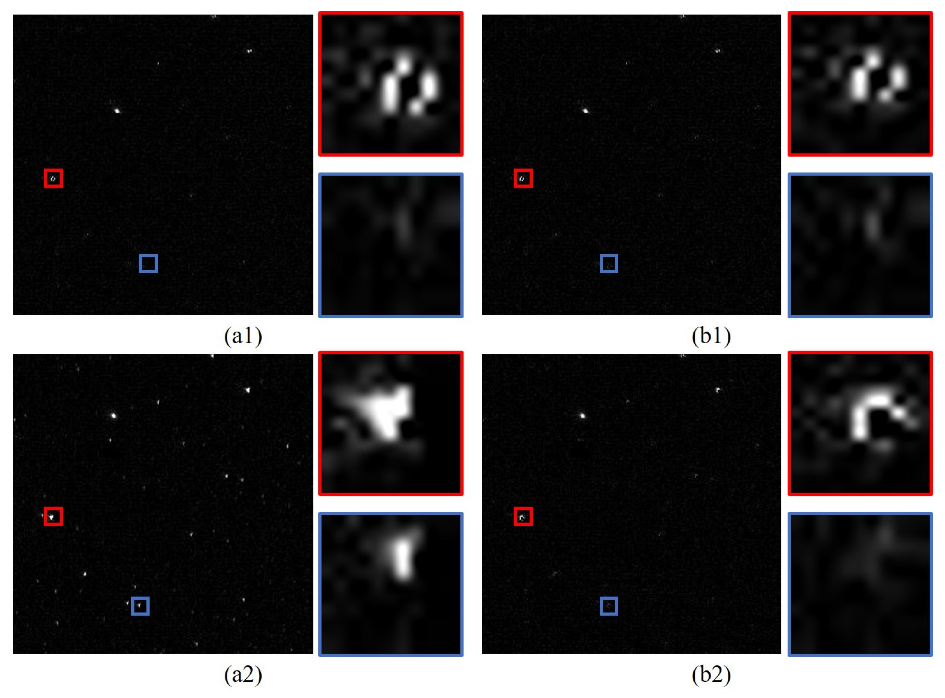
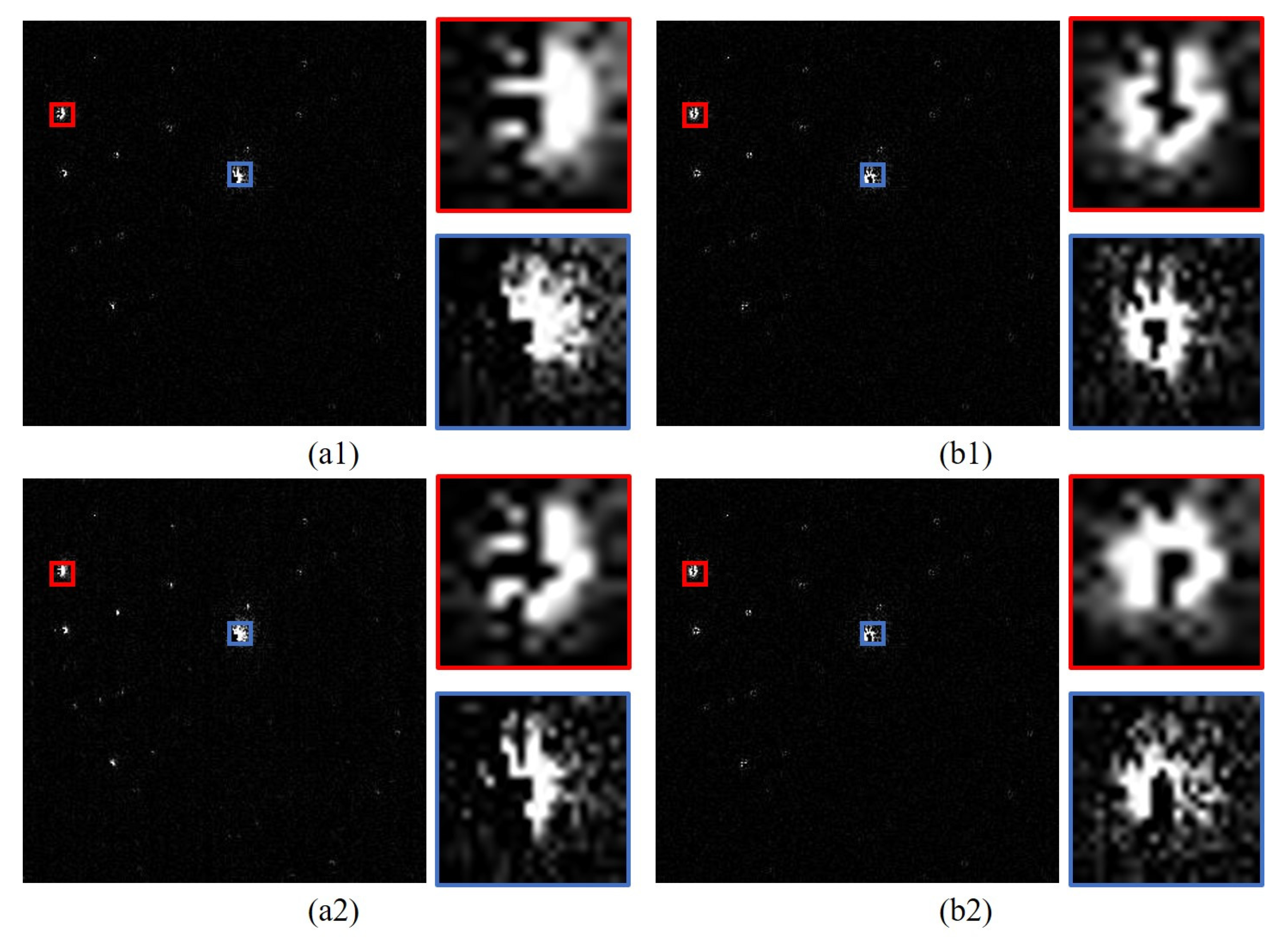
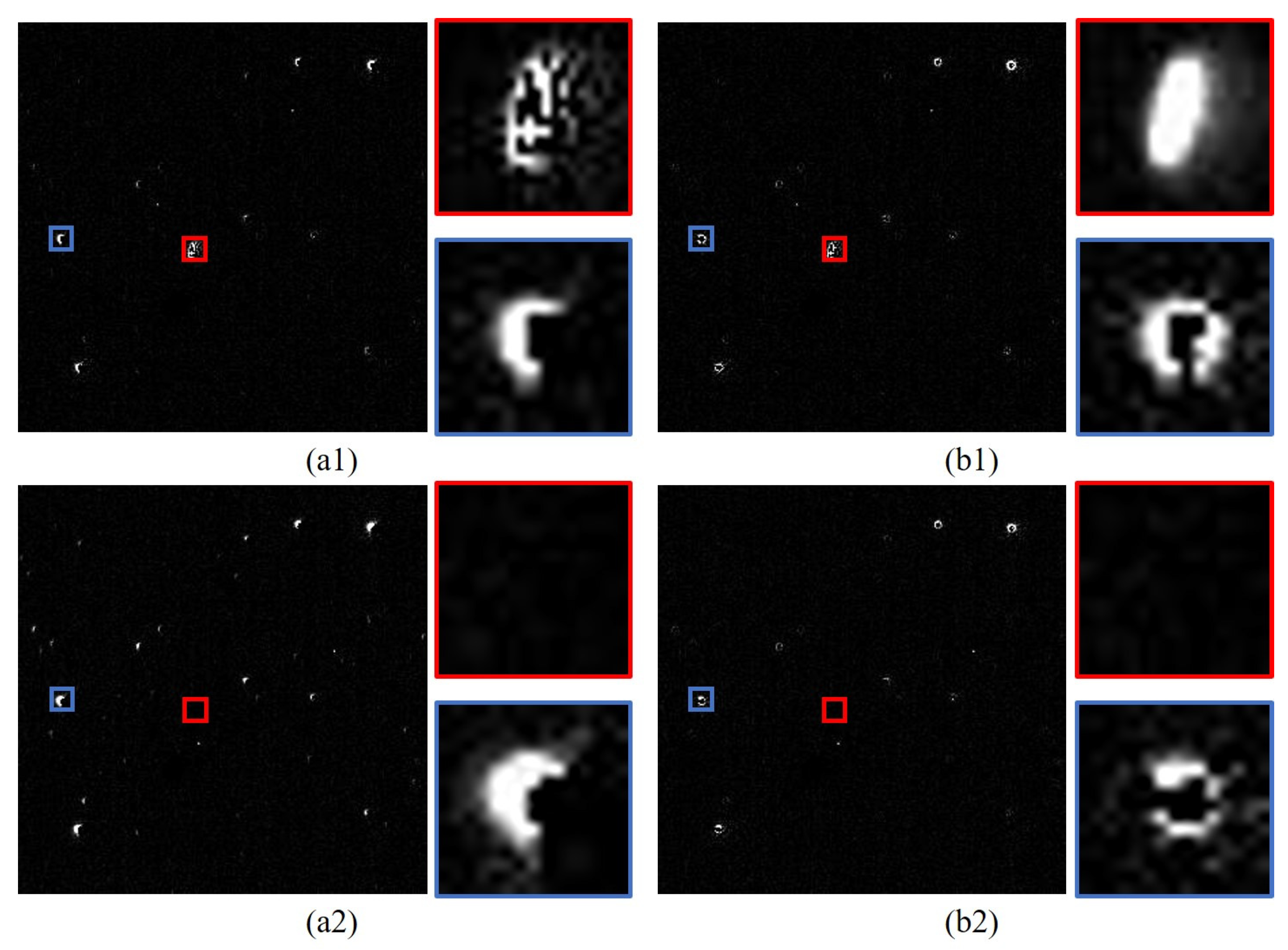
In order to show the differences between the two registration models, the second image and the tenth image in Seq.1 were registered to the reference image, using the proposed method in different transformations. Three regions in the registered images and the reference image were randomly selected, as shown in Figure 8, Figure 9 and Figure 10. In each region, two typical areas, marked in red and blue rectangles, were selected and enlarged. Among them, the red area in Figure 10(a1,b1) was an astronomical image target, so it appeared only once in the same place. The rest of the areas contained only stars.

The location of a region affected the results of the affine transformation, especially when it was a significant distance from the approximate center of rotation, as shown in Figure 9 and Figure 10(a1,a2). Furthermore, when the time interval of two images was small, the differences in registration were not obvious, as shown in Figure 8, Figure 9 and Figure 10(a1,b1). With an increase in time, Figure 8, Figure 9 and Figure 10(a2,b2) show that the deviation of the registered images could not be ignored. Furthermore, Figure 11 shows the influence of the time interval on the different registration models. The pixel error of the matched points was correlated positively with the time interval when using the affine transformation, in all sequences. Because the longer time interval indicated a larger rotation angle of the platform, the affine transformation was not in accord with actual in-orbit conditions. In contrast, the performances of the homography transformations were more stable, which further illustrated the effectiveness of the proposed registration model. Furthermore, the error of our method was also affected by the size of the images and the movements of the stars between two images. If the size was small and the movements were significant, the matched points in the image to be registered would move outward from the same region with increased time intervals, which resulted in fewer points that could be matched and worsening results in the estimation, such as in Seq.6.

The final objective of our study, was to improve target detection in astronomical images. In addition to reducing the influence of the stars, the revision of the target trajectories was another important factor to consider. The trajectories before and after fitting are shown in Figure 12. The typical statistical indices are listed in

Table 7. Comparison of trajectory fitting by different transformations.

Target	Transformation	Mean of Pixel Error
		SSE	R-Squared	RMSE
1	Affine transformation	26.95	1.00	1.13
	Homography transformation	10.10	1.00	0.69
2	Affine transformation	37.71	1.00	1.18
	Homography transformation	18.08	1.00	0.82
3	Affine transformation	497.61	1.00	4.37
	Homography transformation	155.37	1.00	2.44
4	Affine transformation	12.12	1.00	0.67
	Homography transformation	8.08	1.00	0.54
5	Affine transformation	28.43	0.99	1.22
	Homography transformation	15.65	0.99	0.91

. Furthermore, the curvatures of the trajectories revised by two types of transformation are marked in red and green lines, and are shown in Figure 12(b1–b5). The revised trajectories after homography transformation, and the corresponding curves, were smoother, which was advantageous for trace association. The results once again proved the effectiveness of the proposed method.

5. Discussion

A novel registration method for astronomical images was proposed in this paper. There are few studies available in the literature regarding our objectives. The proposed method had better accuracy and speed, as compared to other methods described in Section 1. The advantages and limitations of the presented method are discussed in this section.

1.

The changes in stars in images, caused by the in-orbit motion of platforms, was deduced, to choose the registration model used in this paper. The traditional model was compared to the chosen model, and its limitations were analyzed in detail. The chosen model was more accurate and efficient.

2.

We divided a whole image into regions and used a dynamic threshold based on statistics, to identify the fixed stars easily and efficiently. These stars had a uniform distribution across a whole image, which was advantageous for the parameter estimation of the model.

3.

We utilized the side lengths as the features of the triangles. The side lengths were transformed into relative values, so that the difficulty of threshold setting during the matching of the triangles was reduced and the robustness of the method was improved.

4.

The estimation of parameters included two stages. The traditional model was used to eliminate the wrongly matched points first, because it was more sensitive to these points. The chosen model was applied to realize the accurate registration. Therefore, we eliminated significant errors due to the wrongly matched points, which are typically difficult to directly confirm.

5.

The method involved empirical parameters, one of which was the number of regions. For the same image, a larger number indicated more and smaller regions, which added the burden of high computational demand and the likelihood that the matched points could have moved out of the original region. However, a smaller number could result in an uneven distribution of the selected points. The automatic setting of the regions, combined with the sizes of the images and possible motion of the targets, will be a key factor in our next research focus.

6.

Our purpose in this work was to improve the performance of detection and tracking. In future work, we will propose a new detection and tracking method based on this work, to further expand upon it for potential real-space objects.

6. Conclusions

This paper presented a method for the accurate registration of astronomical images. The central concept of the method was the registration model, sub-regional processing, and the description of the triangle relations of stable stars. Our registration model combined the frequently used affine transformation with a practical in-orbit situation. The proposed method was tested on four sequences of astronomical images, acquired with two astronomical image-based telescopes and a ground-based telescope. By applying strategies for local thresholds and local star matching, the proposed method achieved superior performance for handling large rotation angles, and it had superior resistance to interference, such as stray light and noise. The results also indicated the proposed method was highly competitive in terms of matching accuracy, and it outperformed the baselines for registering astronomical images.

References

1. Felicetti, L.; Emami, M.R. Image-based attitude maneuvers for space debris tracking. Aerosp. Sci. Technol. 2018, 76, 58–71. [Google Scholar] [CrossRef]
2. Furumoto, M.; Sahara, H. Statistical assessment of detection of changes in space debris environment utilizing in-situ measurements. Acta Astronaut. 2020, 177, 666–672. [Google Scholar] [CrossRef]
3. Adushkin, V.; Aksenov, O.Y.; Veniaminov, S.; Kozlov, S.; Tyurenkova, V. The small orbital debris population and its impact on space activities and ecological safety. Acta Astronaut. 2020, 176, 591–597. [Google Scholar] [CrossRef]
4. Marszalek, M.; Rokita, P. Pattern matching with differential voting and median transformation derivation improved point-pattern matching algorithm for two-dimensional coordinate lists. In Computer Vision and Graphics; Springer: Berlin/Heidelberg, Germany, 2006; pp. 1002–1007. [Google Scholar]
5. Tabur, V. Fast Algorithms for Matching CCD Images to a Stellar Catalogue. Publ. Astron. Soc. Aust. 2007, 24, 189–198. [Google Scholar] [CrossRef] [Green Version]
6. Groth, E.J. A pattern-matching algorithm for two-dimensional coordinate lists. Astron. J. 1986, 91, 1244–1248. [Google Scholar] [CrossRef]
7. Stetson, P.B. On the growth-curve method for calibrating stellar photometry with CCDs. Publ. Astron. Soc. Pac. 1990, 102, 932. [Google Scholar] [CrossRef] [Green Version]
8. Valdes, F.G.; Campusano, L.E.; Velasquez, J.D.; Stetson, P.B. FOCAS automatic catalog matching algorithms. Publ. Astron. Soc. Pac. 1995, 107, 1119. [Google Scholar] [CrossRef]
9. Szeliski, R. Image alignment and stitching: A tutorial. Found. Trends Comput. Graph. Vis. 2007, 2, 1–104. [Google Scholar] [CrossRef]
10. Yang, L.; Li, M.; Deng, X. Fast Matching Algorithm for Sparse Star Points Based on Improved Delaunay Subdivision. In Proceedings of the 2nd International Symposium on Computer Engineering and Intelligent Communications (ISCEIC), Nanjing, China, 6–8 August 2021; pp. 117–121. [Google Scholar]
11. Zhou, H.; Yu, Y. Improved Efficient Triangle Similarity Algorithm for Deep-Sky Image Registration. Acta Opt. Sin. 2017, 37, 0410003. [Google Scholar] [CrossRef]
12. Lang, D.; Hogg, D.W.; Mierle, K.; Blanton, M.; Roweis, S. Astrometry. net: Blind astrometric calibration of arbitrary astronomical images. Astron. J. 2010, 139, 1782. [Google Scholar] [CrossRef] [Green Version]
13. Evangelidis, G.D.; Bauckhage, C. Efficient and robust alignment of unsynchronized video sequences. In Pattern Recognition, Proceedings of the 33rd DAGM Symposium, Frankfurt/Main, Germany, 31 August– 2 September 2011; Mester, R., Felsberg, M., Eds.; Lecture Notes in Computer Science; Springer: Berlin/Heidelberg, Germany, 2011; pp. 286–295. [Google Scholar]
14. Lee, M.H.; Cho, M.; Park, I.K. Feature description using local neighborhoods. Pattern Recognit. Lett. 2015, 68, 76–82. [Google Scholar] [CrossRef]
15. Keller, W.A. Inside PixInsight; Springer: Berlin/Heidelberg, Germany, 2016. [Google Scholar]
16. Zhou, H.; Yu, Y. Applying rotation-invariant star descriptor to deep-sky image registration. Front. Comput. Sci. 2018, 12, 1013–1025. [Google Scholar] [CrossRef]
17. Lowe, D.G. Distinctive image features from scale-invariant keypoints. Int. J. Comput. Vis. 2004, 60, 91–110. [Google Scholar] [CrossRef]
18. Bay, H.; Ess, A.; Tuytelaars, T.; Van Gool, L. Speeded-up robust features (SURF). Comput. Vis. Image Underst. 2008, 110, 346–359. [Google Scholar] [CrossRef]
19. Mikolajczyk, K.; Schmid, C. A performance evaluation of local descriptors. IEEE Trans. Pattern Anal. Mach. Intell. 2005, 27, 1615–1630. [Google Scholar] [CrossRef] [PubMed] [Green Version]
20. Rublee, E.; Rabaud, V.; Konolige, K.; Bradski, G. ORB: An efficient alternative to SIFT or SURF. In Proceedings of the 2011 International Conference on Computer Vision, Barcelona, Spain, 6–13 November 2011; pp. 2564–2571. [Google Scholar]
21. Leutenegger, S.; Chli, M.; Siegwart, R.Y. BRISK: Binary robust invariant scalable keypoints. In Proceedings of the 2011 International Conference on Computer Vision, Barcelona, Spain, 6–13 November 2011; pp. 2548–2555. [Google Scholar]
22. Alahi, A.; Ortiz, R.; Vandergheynst, P. Freak: Fast retina keypoint. In Proceedings of the 2012 IEEE Conference on Computer Vision and Pattern Recognition, Providence, RI, USA, 16–21 June 2012; pp. 510–517. [Google Scholar]
23. Alcantarilla, P.F.; Bartoli, A.; Davison, A.J. KAZE features. In Computer Vision, Proceedings of the 12th European Conference on Computer Vision, Florence, Italy, 7–13 October 2012; Fitzgibbon, A., Lazebnik, S., Perona, P., Sato, Y., Schmid, C., Eds.; Lecture Notes in Computer Science; Springer: Berlin/Heidelberg, Germany, 2012; pp. 214–227. [Google Scholar]
24. Dalal, N.; Triggs, B. Histograms of oriented gradients for human detection. In Proceedings of the 2005 IEEE Computer Society Conference on Computer Vision and Pattern Recognition (CVPR’05), San Diego, CA, USA, 20–25 June 2005; Volume 1, pp. 886–893. [Google Scholar]
25. Ruiz-del Solar, J.; Loncomilla, P.; Zorzi, P. Applying SIFT descriptors to stellar image matching. In Progress in Pattern Recognition, Image Analysis and Applications, Proceedings of the 13th Iberoamerican Congress on Pattern Recognition, CIARP 2008, Havana, Cuba, 9–12 September 2008; Springer: Berlin/Heidelberg, Germany, 2008; pp. 618–625. [Google Scholar]
26. DeTone, D.; Malisiewicz, T.; Rabinovich, A. Deep image homography estimation. arXiv 2016, arXiv:1606.03798. [Google Scholar]
27. Le, H.; Liu, F.; Zhang, S.; Agarwala, A. Deep homography estimation for dynamic scenes. In Proceedings of the IEEE/CVF Conference on Computer Vision and Pattern Recognition, Seattle, WA, USA, 13–19 June 2020; pp. 7652–7661. [Google Scholar]
28. Nguyen, T.; Chen, S.W.; Shivakumar, S.S.; Taylor, C.J.; Kumar, V. Unsupervised deep homography: A fast and robust homography estimation model. IEEE Robot. Autom. Lett. 2018, 3, 2346–2353. [Google Scholar] [CrossRef] [Green Version]
29. Zhang, J.; Wang, C.; Liu, S.; Jia, L.; Ye, N.; Wang, J.; Zhou, J.; Sun, J. Content-aware unsupervised deep homography estimation. In Computer Vision—ECCV 2020, Proceedings of the 16th European Conference, Glasgow, UK, 23–28 August 2020; Vedaldi, A., Bischof, H., Brox, T., Frahm, J.M., Eds.; Lecture Notes in Computer Science; Springer: Berlin/Heidelberg, Germany, 2020; pp. 653–669. [Google Scholar]
30. Ye, N.; Wang, C.; Fan, H.; Liu, S. Motion basis learning for unsupervised deep homography estimation with subspace projection. In Proceedings of the IEEE/CVF International Conference on Computer Vision, Montreal, BC, Canada, 11–17 October 2021; pp. 13117–13125. [Google Scholar]
31. Sedaghat, A.; Mokhtarzade, M.; Ebadi, H. Uniform robust scale-invariant feature matching for optical remote sensing images. IEEE Trans. Geosci. Remote. Sens. 2011, 49, 4516–4527. [Google Scholar] [CrossRef]
32. Tuytelaars, T.; Mikolajczyk, K. Local invariant feature detectors: A survey. Found. Trends Comput. Graph. Vis. 2008, 3, 177–280. [Google Scholar] [CrossRef] [Green Version]
33. Markwardt, C.B. Non-linear least squares fitting in IDL with MPFIT. arXiv 2009, arXiv:0902.2850. [Google Scholar]
Figure 1. An in-orbit satellite under typical conditions. (a) Position change. (b) Influence of (a) on imaging.
Remotesensing 15 01921 g001
Figure 2. An illustration of triangle construction in two images for registration. (a) Reference image. (b) Current image. (c) Photomicrographs of the marked region in (a). (d) Photomicrographs of the marked region in (b).
Remotesensing 15 01921 g002
Figure 3. The simulation of points in the 1500 × 1500 image.
Remotesensing 15 01921 g003
Figure 4. The range of the relative variation in lengths.
Remotesensing 15 01921 g004
Figure 5. Real astronomical image sequences. (a) Seq.1, (b) Seq.2, (c) Seq.3, (d) Seq.4, (e) Seq.5, and (f) Seq.6.
Remotesensing 15 01921 g005
Figure 6. Original targets in sequences. (a1d1) Target 1. (a2d2) Target 2. (a3d3) Target 3. (a4d4) Target 4. (a5d5) Target 5.
Remotesensing 15 01921 g006
Figure 7. The results of matching for two images in Seq.2. (a) SURF. (b) Global threshold + improved SURF. (c) ORB. (d) Global threshold + Delaunay. (e) Ours.
Remotesensing 15 01921 g007
Figure 8. Region 1 in the difference images using (a) affine transformation and (b) homography transformation. (a1,b1) The difference image of the second frame and the reference image. (a2,b2) The difference image of the tenth image and the reference image.
Remotesensing 15 01921 g008
Figure 9. Region 2 in the difference images using (a) affine transformation and (b) homography transformation. (a1,b1) The difference image of the second frame and the reference image. (a2,b2) The difference image of the tenth image and the reference image.
Remotesensing 15 01921 g009
Figure 10. Region 3 in the difference images using (a) affine transformation and (b) homography transformation. (a1,b1) The difference image of the second frame and the reference image. (a2,b2) The difference image of the tenth image and the reference image.
Remotesensing 15 01921 g010
Figure 11. The error curve of difference transformation for matched points in (a) Seq.1, (b) Seq.2, (c) Seq.3, (d) Seq.4, (e) Seq.5, and (f) Seq.6.
Remotesensing 15 01921 g011
Figure 12. The results of (a1a5) fitting trajectories and (b1b5) corresponding curvature changes in different sequences.
Remotesensing 15 01921 g012