Article

Landslide Susceptibility Mapping and Driving Mechanisms in a Vulnerable Region Based on Multiple Machine Learning Models

1
State Key Laboratory of Subtropical Silviculture, Zhejiang A&F University, Hangzhou 311300, China
2
College of Environmental and Resource Sciences, Zhejiang A&F University, Hangzhou 311300, China
*
Author to whom correspondence should be addressed.
These authors contribute equally to this work.
Remote Sens. 2023, 15(7), 1886; https://doi.org/10.3390/rs15071886
Submission received: 22 February 2023 / Revised: 21 March 2023 / Accepted: 29 March 2023 / Published: 31 March 2023
(This article belongs to the Special Issue Advancement of Remote Sensing in Landslide Susceptibility Assessment)

Abstract

:
Landslides can cause severe damage to both the environment and society, and many statistical, index-based, and inventory-based methods have been developed to assess landslide susceptibility; however, it is still challenging to choose the most effective method and properly identify major driving factors for specific regions. Here, we applied four machine learning algorithms, adaptive boosting (AdaBoost), gradient-boosting decision tree (GBDT), multilayer perceptron (MLP), and random forest (RF), to predict the landslide susceptibility at 30 m spatial scale based on thirteen landslide conditioning factors (LCFs) in a landslide-vulnerable region. Based on inventory landslide points, the classification results were evaluated, and indicated that the performance of the RF (F1-score: 0.85, AUC: 0.92), AdaBoost (F1-score: 0.83, AUC: 0.91), and GBDT (F1-score: 0.83, AUC: 0.88) methods were significantly better than the MLP (F1-score: 0.76, AUC: 0.79) method. The results further indicated that the areas with high and very high landslide risk (susceptibility greater than 0.5) accounted for about 40% of the study region. All four models matched well and predicted similar spatial distribution patterns in landslide susceptibility, with the very high risk areas mostly distributed in the western and southeastern regions. Daoshi, Qingliangfeng, Jinnan, and Linglong towns have the highest landslide risk, with mean susceptibility levels greater than 0.5. The leading contributing factors to landslide susceptibility were slightly different for the four models; however, population density, distance to road, and relief amplitude were generally among the top leading factors for most towns. Our study provided significant information on the highly landslide-prone areas and the major contributing factors for decision-makers and policy planners, and suggested that different areas should take unique precautions to mitigate or avoid severe damage from landslide events.

1. Introduction

Landslides are considered a natural hazard that causes extensive damage to the environment and societies. A landslide hazard map demonstrates regions susceptible to landslides by considering the phenomenon’s causative and triggering factors (e.g., geomorphological, geological, and meteorological) [1]. Landslide susceptibility is the likelihood of landslides occurring based on local topographical conditions [2]. Various approaches to landslide susceptibility mapping (LSM) have been proposed and practiced during the last few decades [3]. These methods can be broadly divided into five categories: geomorphological mapping, analysis of inventories, index-based approaches, process-based methods, and statistical modeling methods [3]. Among the statistical modeling methods, machine learning methods, a powerful group of data-driven tools, have experienced an increasing preference in recent years [4].
Machine learning methods have shown the inherent and unique advantages of a data-driven model, which can deeply mine effective information on big data and avoid starting with an assumed structural model, and thus excel in the field of modeling [4,5]. Felicísimo et al. [6] indicated that the most important factor that determines the accuracy of the LSMs is the selection of the best machine learning techniques. Owing to its superiority demonstrated for exploratory data analysis, support vector machine (SVM) [7,8,9,10,11], multilayer perceptron (MLP) [12,13,14], artificial neural network (ANN) [5,13,15,16,17,18,19,20], and random forest (RF) [21,22,23,24,25] have been widely used in LSM. These types of models are an advanced optimization of decision-making algorithms such as the analytic hierarchy process (AHP), K-L information value method, and weighted linear combination model [26]. In recent years, ensemble-based machine learning methods have emerged in LSM because they can improve the model prediction capability, and manage complex multidimensional data [27,28]. This method applies a combination of various classifiers to predict LSM. Various ensemble-based methods have been proposed and applied, such as adaptive boosting (AdaBoost) [17,18,29], gradient-boosting decision tree (GBDT) [19,20], and rotation forest [30]. All of these machine-learning methods have been proved effective in different studies; however, some methods may be more effective and outperform others in specific regions [31]. For example, Ng et al. [32] found that RF has better performance than the MLP, AdaBoost, or SVM methods in predicting rainfall-induced landslides, while Tien Bui et al. [33] indicated that the MLP method outperformed several other traditional machine learning models. Therefore, disagreement still exists on which method is the best for the prediction of landslide susceptibility at regional scale [33,34]. Even 1 or 2% increase in the prediction accuracy could significantly affect the resulting LSM [35], and therefore it is necessary to compare and choose the highest performance models [33].
Understanding the relationship between landslides and their driving mechanisms forms the basis for predicting future landslides and assessing landslide hazards [36,37,38]. Many geoenvironmental factors have been selected as variables in predicting landslide susceptibility, including soil condition (e.g., soil texture, soil type, and soil depth), root strength, bedrock (e.g., lithology), topography (e.g., slope, distance to fault, aspect, and elevation), hydrology (e.g., distance to river and groundwater depth), climate (e.g., rainfall and snowmelt velocity), land use and land cover (e.g., crop fraction and vegetation coverage), and human activities (e.g., distance to road and infrastructure fraction) [3,38,39,40,41,42,43]. The identified leading landslide condition factors (LCFs) vary greatly in different study regions and when using different prediction methods. For example, using multiple decision-tree machine learning methods, Hong et al. [28] found that slope, land cover, and lithology are the top three LCFs in Jiangxi Province. Based on deep learning and conventional machine learning models, Bui et al. [44] found that elevation, slope, soil, and lithology are the major contributing LCFs in Kon Turn Province, Viet Nam. Based on different hybrid machine learning methods, Chen and Li [18] concluded that slope, land cover, distance to roads, and elevation are the leading LCFs in Chongqing City, China; while using similar hybrid methods, their another study [45] indicated that distance to road, elevation, distance to river, and land cover are the major LCFs in Shaanxi Province. These previous studies have obtained different conclusions concerning major contributing factors at various scales that could be due to the complex nature of landslides [33,46]; thus, producing a reliable spatial prediction of landslides remains a challenging task [31].
The Lin’An District is located at the west of Hangzhou City in Zhejiang Province, China. Frequent landslide events occurred in this region due to heavy rainfall resulted from typhoons, mountainous terrains with high slopes, fractured geological formations and lithology, well-weathered soil, and intensive human activities. To date, no studies have reported the spatiotemporal characteristics and susceptibility of landslides specifically for this region. Many studies have applied conventional machine learning methods to study LSM, while the ensemble-based machine learning methods are novel and have been less applied. More studies are needed to evaluate their performance against the conventional machine learning methods. To avoid or reduce the ecological, economic, and life losses from landslides and maintain sustainable development, it is urgent to provide the extent and intensity of landslide susceptibility and identify underlying contributing factors, which could help policy-makers reduce or avoid the occurrence of disasters in advance or rescue the environment after disasters. Therefore, our main objectives are to (1) compare the performance of four machine learning algorithms, MLP, AdaBoost, GBDT, and RF, in landslide susceptibility prediction; (2) explore the pixel- (30 m) and town-level patterns of high-risk landslide areas; and (3) identify the major contributing factors to landslide susceptibility at regional and town levels.

2. Methodology

2.1. Study Region

The case study region is located in the Lin’An District (29°56′–30°23′ N, 118°51′–119°52′ E), Hangzhou City, Zhejiang Province, China (Figure 1). This region is about 100 km wide from east to west, and about 50 km long from north to south, and with a total area of 3127 km2. This region belongs to the subtropical monsoon climate zone. The average annual precipitation is 1614 mm and mostly occurs in summer [47]. The extreme climate events such as strong wind, extreme rainfall events, and typhoons frequently occur. The terrain slopes decline from the west to southeast, and this region is surrounded by high mountains on the north, west, and southeast. The elevation of the eastern valley plain is generally below 50 m above sea level, with the lowest at 4 m below sea level in Qingshanhu town, while the highest elevation is 1787 m in the western Qingliang Mountains. The study region was reported to be vulnerable to landslides due to the high frequency of extreme rainfall and wind events, high slopes, the undulatory terrains, fractured geological formation and lithology, well-weathered soil, and improper human construction (e.g., roads and villages).

2.2. Data Description

2.2.1. Model Input Variables and Descriptions

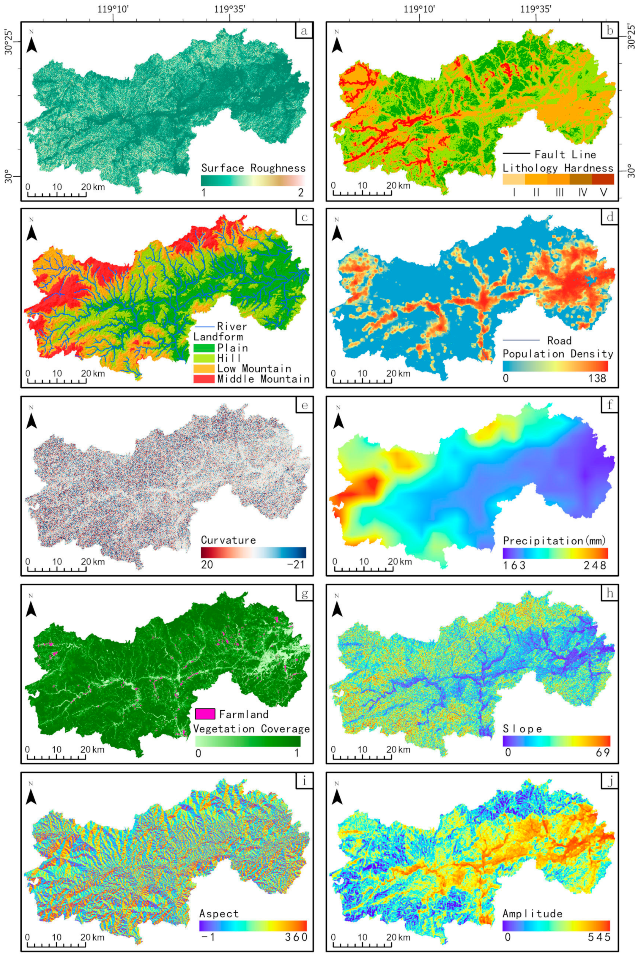
The identification of the main controlling factors of landslide disasters plays an indispensable role in landslide occurrence prediction and risk assessment [41]. Generally, the influencing factors are divided into stable condition factors and triggering condition factors [48], and stable conditions can be further divided into material conditions and topographic conditions [42]. In this study, we mainly selected the stable condition factors, because our assessment emphasizes the possibility of landslides under long-term stable geological conditions, while the triggering condition factors mainly emphasize the possibility of disasters under a short-term influence [43]. Based on previous research, thirteen landslide condition factors were selected, including slope, aspect, curvature, surface roughness, relief amplitude, landform, lithology, vegetation coverage, distance to fault, distance to road, distance to river, population density, and precipitation (average monthly precipitation). The data sources and characteristics are shown in Table 1, and the spatial distribution patterns of some key factors are shown in Figure 2.
Among the input variables, monthly precipitation in the study region ranges from 163 to 248 mm, with a declining tendency from the west to the east. The extremely high monthly rainfall can be over 400 mm in some years with super strong typhoons, such as during the period of Typhoon Lekima in August 2019. Lithology is divided into I to V grades in terms of hardness, representing rock hardness and structural integrity [49]. Landforms are divided into six categories: plain (elevation < 200 m), hill (201–500 m), low mountain (501–1000 m), middle mountain (1001–3500 m), high mountain (3501–5000 m), and highest mountain (>5000 m) [50].
The calculation methods for some of the input variables are described here. Vegetation fractional coverage ( V F C ) represents the fraction of vegetation within each pixel. The calculation formula is as follows:
V F C = ( N D V I N D V I s o i l ) / ( N D V I v e g N D V I s o i l )
where N D V I s o i l is N D V I (normalized difference vegetation index) for bare soil, N D V I v e g   i s   N D V I for vegetated areas.
The surface roughness ( D ) is used to reflect surface fluctuation and degree of erosion. It can be expressed as the ratio of the grid surface area to its projected area, which is the reciprocal of the cosine of the slope ( ) after conversion [51]:
D = 1 cos  
Relief amplitude ( R D L S ) reflects the relative height difference in the ground, which is the difference between the maximum elevation ( D E M m a x ) and the minimum elevation ( D E M m i n ) [52]:
R D L S = D E M m a x D E M m i n
The curvature is calculated using the incomplete quartic method [53]. All the above factors were calculated using QGIS software (https://qgis.org/en/site/, accessed on 10 September 2022).

2.2.2. Training and Validation Sample Plot Data

Landslide occurrence points recorded during 1949–2020 were collected from the Resource and Environment Science and Data Center, Chinese Academy of Sciences (https://www.resdc.cn/, accessed on 10 September 2022) (Table 1). This dataset recorded most of the landslide occurrence points in the study region. A landslide occurrence was recorded as “1”. There are 146 landslide occurrence points, indicating 146 landslides occurred during the historical period. We further randomly established 146 points (marked as “0”) to represent points without landslides. We further extracted the data for the 13 model input variables at each sample point (Figure 2). Finally, we obtained a training and validation dataset with 292 sample points (Figure 1). The dataset is further divided into a training and development set and a test set, which are used to train the models and test the accuracy of the models, respectively. The training and development set has 232 sample points (80%) and the test set has 60 sample points (20%).

2.3. Research Work Flow

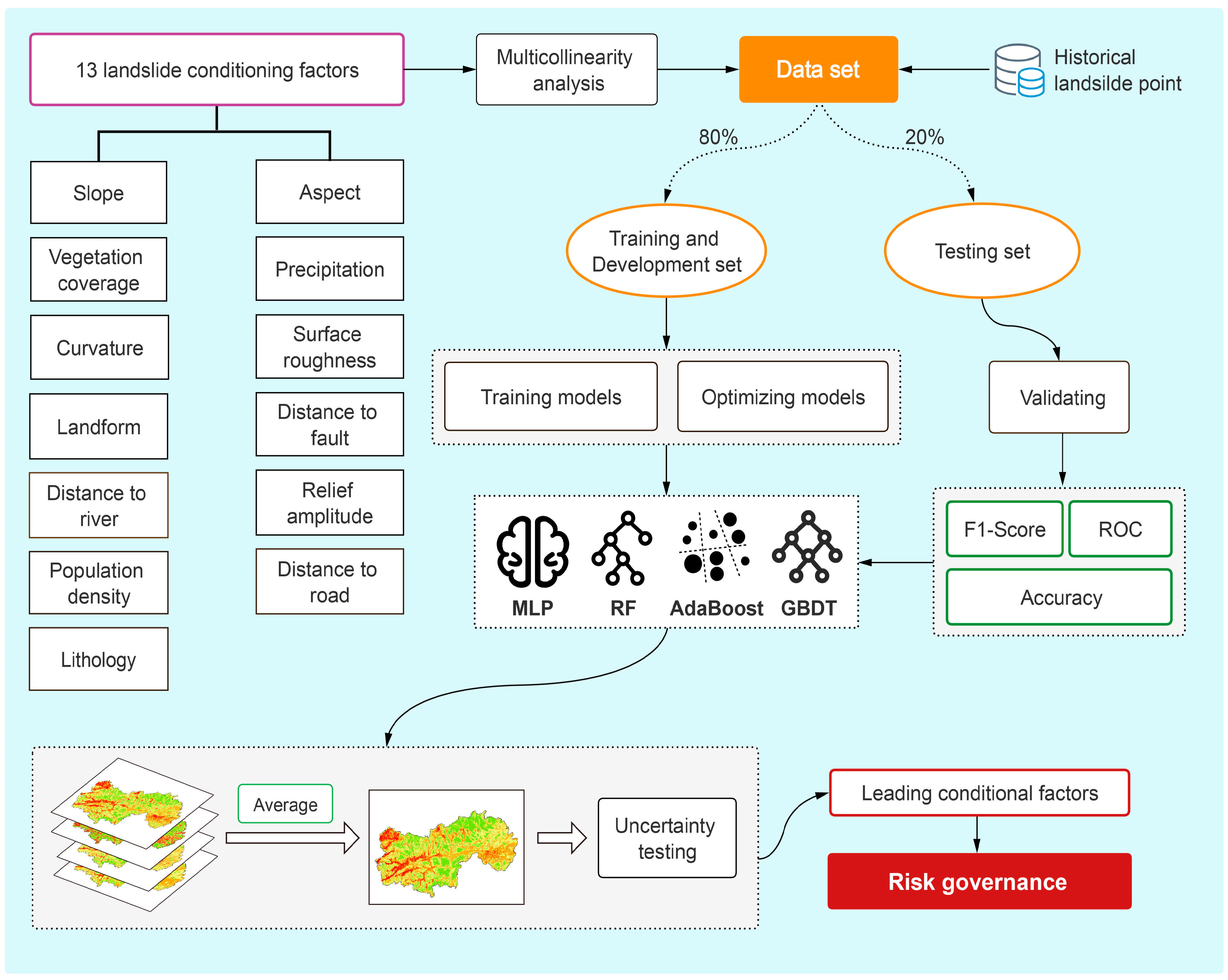
The entire research flow is shown in Figure 3, more detailed processes are described below.

2.3.1. Multicollinearity Test

Before the prediction of landslide susceptibility, the independence of each input variable must be tested. This can not only reduce the amount of data but also improve the accuracy of the prediction models. The variance inflation factor (VIF) and tolerance (TOL) were used to screen all 13 input variables for multicollinearity [54,55,56]. VIF represents the ratio of the variance of the regression coefficient estimator to the variance assuming a nonlinear correlation between independent variables, and TOL is the inverse of the VIF value, both of which can test the multicollinearity between variables. In general, VIF >10 and TOL <0.1 indicate a serious multicollinearity problem between variables [57].

2.3.2. Adaptive Boosting (AdaBoost) Method

The adaptive boosting algorithm is one of the most popular methods in the integrated learning-boosting methods, which was first proposed by Freund and Schapire [58]. Schapire proved that strong and weak learning algorithms are equivalent [59], Therefore, several weak learning algorithms can be constituted into a strong learning algorithm. AdaBoost is a boosting algorithm that combines a series of weak classifiers into a strong classifier [60]. Firstly, the algorithm initializes the weight distribution of the training data and trains each weak classifier. Then, it calculates the classification error between its classification result and the training data. Finally, it updates the weight distribution for the training dataset according to the classification error rate. In each round of calculation, the weight value of the samples classified incorrectly in the previous round increases, and the weight value of the samples correctly classified decreases, so that the later classifiers give more attention to the samples that are classified incorrectly in the previous round. Eventually, AdaBoost obtains the final classification result through weighted calculation [60]. In this study, we take the decision-tree classifier as the basic classifier of the AdaBoost algorithm. Compared with other weak classifiers, the decision tree with AdaBoost model has faster calculation speed and better performance in large-scale data training [61].

2.3.3. Gradient-Boosting Decision-Tree (GBDT) Method

The gradient-boosting algorithm was proposed by Freidman in 2001 [62]. Gradient boosting is a large class of algorithms in boosting. GBDT is a gradient-boosting algorithm that uses decision trees as weak classifiers. The idea of gradient boosting is based on the gradient-descent method, which reduces a loss by fitting the residual of the previous time to achieve the purpose of joint decision-making. The basic principle of GBDT is to train the weak classifiers according to the negative gradient information from the current model loss function, and then add the weak classifiers to the existing model. It has good interpretability and robustness, and is considered as an algorithm with strong generalization ability and wide application [63].

2.3.4. Multilayer Perceptron Method

MLP is the most common fully connected artificial neural network (ANN), which is generally considered to be a model that uses a hyperplane to classify the feature vector x of an input instance [12]. The model has multiple layers, including an input layer, an output layer, and one or more hidden layers [64,65]. In each layer, the neurons usually contain a linear function and a nonlinear activation function, and the weight coefficient W and bias b in the linear function are adjusted by the gradient-descent algorithm [66] to make the value of the loss function reach a minimum. In this study, the sigmoid function was used as the activation function for the output layer so that the result of the output layer can be regarded as the probability of classification in the binary classification model.

2.3.5. Random Forest Method

The random forest (RF) classifier is several decision trees constructed by bootstrapping [67], which has a better generalization ability than other traditional mathematical models when dealing with high-dimensional samples, and has been widely used in geological disaster prevention research. The randomness of the random forest is reflected in the sampling process and feature selection. The random forest obtains N independent samples as the training samples of the ith ( 1 i N ) decision tree of the random forest by performing random sampling with a replacement for n times. Since each sampling is an independent random event with replacement, according to the limit formula (Equation (4)), about one-third of the samples each time do not appear in the selected sample set.
lim N   1 + 1 N N = lim N   1 ( N N 1 ) N = lim N   1 ( 1 + 1 N 1 ) N = 1 e
The performance of the model is affected by the training process, such as the number of submodels and learning rate, and is also affected by the performance of submodels, such as maximum tree depth and criterion.

2.3.6. Model Parameterization

The four models should be first optimized by selecting the appropriate hyperparameters. Commonly used hyperparameter optimization methods include grid search, cross-validation, and random search [68,69]. In this study, grid search and K-fold cross-validation were applied to select the optimal hyperparameters for the models in the training–development set (Table 2). These optimal hyperparameters are obtained by achieving the highest mean testing accuracy in K-fold validation. The hidden layer for MLP is set to one layer containing four neurons with the Adam optimizer as its optimization algorithm. Epoch refers to how many cycles through the full training dataset, and batch size represents the number of samples per gradient update. The RF method uses a total of 17 trees, 3 maximum feature numbers for each tree, and 3 minimum numbers of samples. AdaBoost and GBDT use 40 and 17 trees, respectively. The more trees denote a more complex model and more powerful ability of data training. However, too many trees are prone to be overfiting when the models are trained by a small dataset. Considering our training data size, we established these parameters for four methods.

2.3.7. Model Evaluation Metrics

In this study, the overall accuracy (OA), F1-score, and AUC (ROC curve) were used to evaluate the performance of the modeling results. F1-score is a precision evaluation index that unifies precision and recall. It is widely used in the precision evaluation of machine learning models [70,71]. Firstly, we need to use the confusion matrix to calculate the precision and recall. The precision rate is the proportion of samples that are actually positive among all the samples and are also predicted to be positive (Equation (5)). The recall rate is the proportion of the correct sample predicted in the actual positive class sample (Equation (6)). F1-score is actually a harmonic mean of precision and recall (Equation (7)).
P r e c i s i o n % = T P T P + F P × 100 %
R e c a l l % = T P T P + F N × 100 %
F 1 - S c o r e = 2 × p r e c i s i o n × r e c a l l p r e c i s i o n + r e c a l l
A c c u r a c y = T P + T N T P + T N + F P + F N
where TP is true positive sample numbers; FP is false positives; FN is false negatives; TN is true negatives.
The receiver-operating characteristic curve (ROC) takes each value of the prediction result as a possible judgment threshold. With the false positive rate (FPR) as the X-axis (Equation (9)) and the true positive rate (TPR) as the Y-axis (Equation (10)), the ROC curve is calculated by connecting the corresponding points of the samples distributed among the coordinate system:
F P R = F P F P + T N
T P R = T P T P + F N
The larger the FPR on the horizontal axis, the more actual negative classes in the predicted positive class, and the larger the TPR on the vertical axis, the more actual positive classes in the predicted positive class. The ideal prediction situation is FPR equal to 0 and TPR equal to 1, which corresponds to the (0, 1) point in the coordinate axis. As an evaluation metric measuring the accuracy of the classification model, the area under the curve (AUC) for an actual classifier is between 0.5 and 1 [72]. For example, a landslide prediction model has a false positive rate prediction that indicates the probability of a landslide occurring where it did not actually occur, and a true positive rate indicated the probability that a landslide would actually occur. The closer the ROC curve radian is to the (0, 1) point, that is, the closer the AUC value is to 1, the better the prediction effect [73].

3. Results and Analysis

3.1. Multicollinearity Analysis

Multicollinearity among the condition factors were identified using the variance inflation factors (VIF) and tolerances (TOL). The results showed that the largest VIF value was 4.98 from landform, which is lower than the collinearity threshold of 10 (Table 3). The lowest tolerance was 0.20, also from landform, which is greater than the collinearity threshold of 0.1. Both indicators suggest that all thirteen factors did not have serious collinearity problems, and can be used as input variables for the four models.

3.2. Accuracy Assessment for the Modeling Results

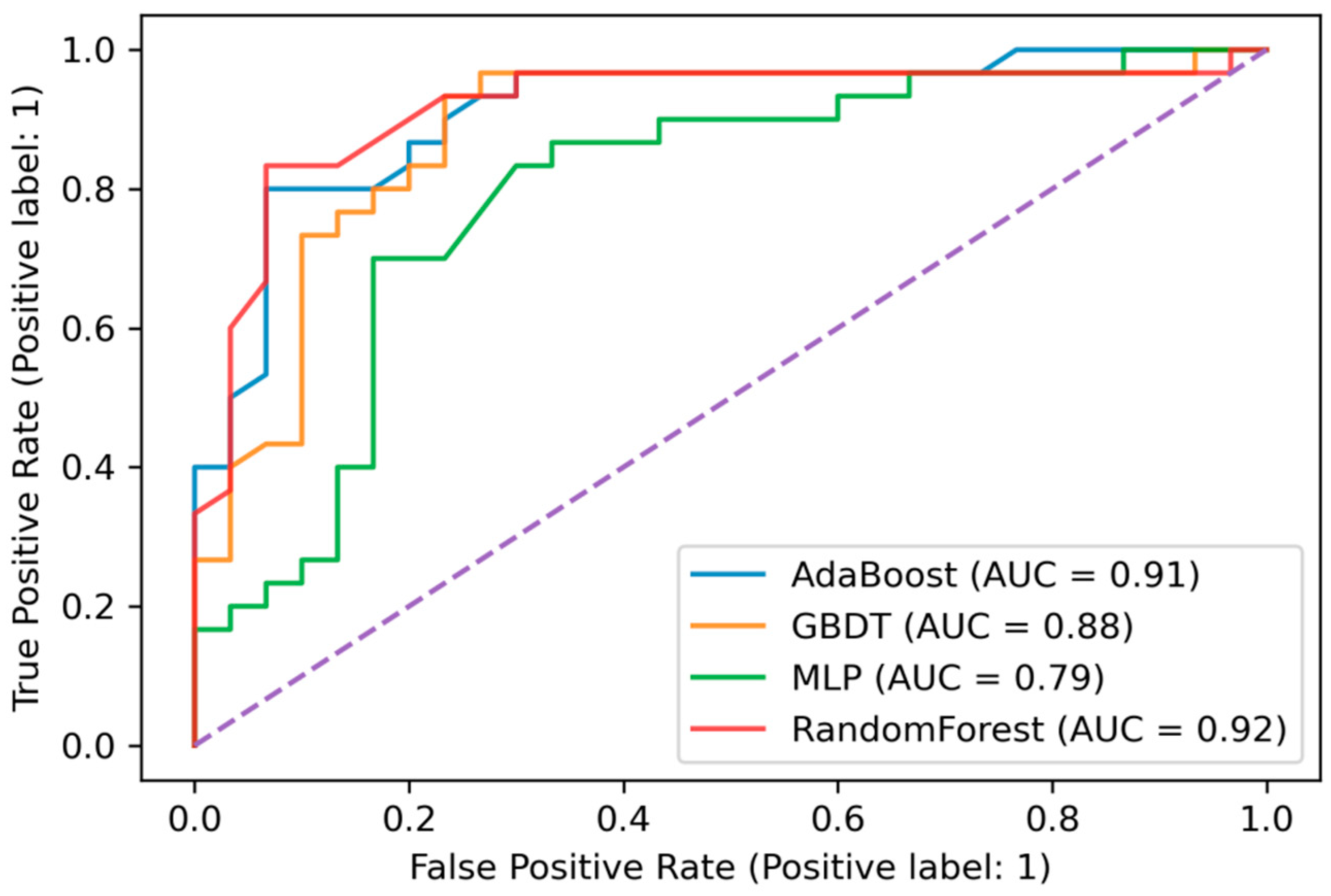
The estimated landslide susceptibility from the four machine learning methods was evaluated against the sampling plot data based on the F1-score and AUC values. In terms of F1-score, the results indicated that the accuracy of RF (F1-score = 0.85), AdaBoost (F1-score = 0.83), and GBDT (F1-score = 0.83) were similar, but all significantly higher than MLP (0.77) (Table 4). In terms of the AUC values, all the models exhibited a sufficient performance (AUC >0.79). The success rate and generalization ability of RF (0.92), AdaBoost (0.91), and GBDT (0.88) were also significantly higher than MLP (Figure 4). Overall, the RF model had the best performance for predicting landslide susceptibility, followed by AdaBoost and GBDT, with the worst from MLP. The evaluations also indicated that all models selected in this study have reasonable goodness-of-fit in spatial prediction of landslide susceptibility.
At spatial scale, the predictive differences among four models were also quantitatively evaluated by cross-correlation coefficient (Table 5). The results showed that the correlation coefficients between MLP and other three models were generally lower than 0.74, while the correlation coefficients among RF, AdaBoost and GBDT were higher than 0.88. This implied that the three methods based on decision trees generally performs better. Overall, the modeling results of the integrated model used in the study have relatively high spatial similarity, which further mutually proved the effectiveness of the model prediction results.

3.3. Predicted Landslide Susceptibility

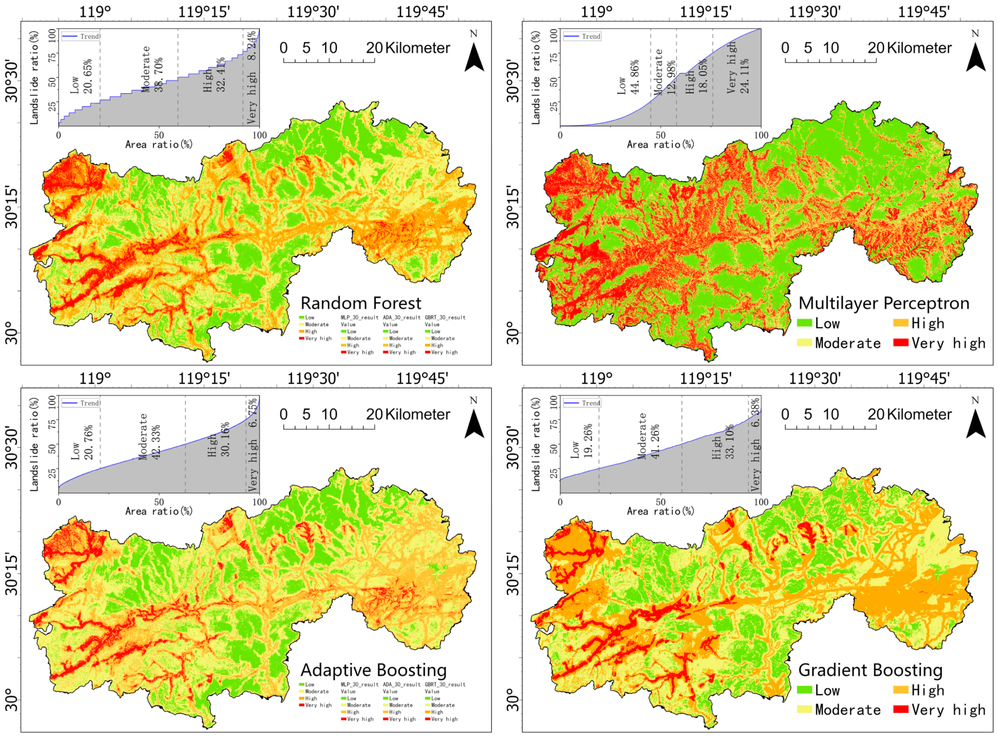
The four models evaluated were used to assess landslide susceptibility in the study area. The landslide susceptibility was regrouped into five susceptibility classes: very high prone (0.75~1.00), high (0.50~0.75), moderate (0.25~0.50), and low (0~0.25) (Table 6). Overall, the distribution of landslide susceptibility for each class was similar among the four methods. The “very high” susceptibility class covered about 8%, 24%, 7%, and 7% of the total area based on the RF, MLP, AdaBoost, and GBDT models, respectively. The “low” susceptibility class covered about 21%, 45%, 21%, and 19% of the total area based on the RF, MLP, AdaBoost, and GBDT models, respectively. Totally, the “high” and “very high” classes accounted for about 40%, 42%, 37%, and 40% of the total land area based on the RF, MLP, AdaBoost, and GBDT models, respectively, with a mean high-risk fraction of 40%. Overall, the three decision-tree-based methods (RF, AdaBoost, and GBDT) had very similar prediction for all four categories, while the MLP method predicted a significantly higher fraction of “low” and “very high” risk area. At town level, the mean landslide susceptibility values in Qingliangfeng (0.53), Daoshi (0.66), Jinnan (0.61), and Linglong (0.58) towns were distributed in the range for the “high prone” class, indicating these towns are more vulnerable to landslide incidence (Table 7). Most of the other towns have “moderate prone” landslide risk. Among the four highest risk towns, Daoshi had the highest fraction (37.56) of “very high” risk area, while Linglong had the highest fraction (68.92%) of “high” risk area. This indicates that the high overall landslide susceptibility in Daoshi mostly results from the “very high” risk fraction, while in Linglong it results from the “high” risk fraction (Table 7).
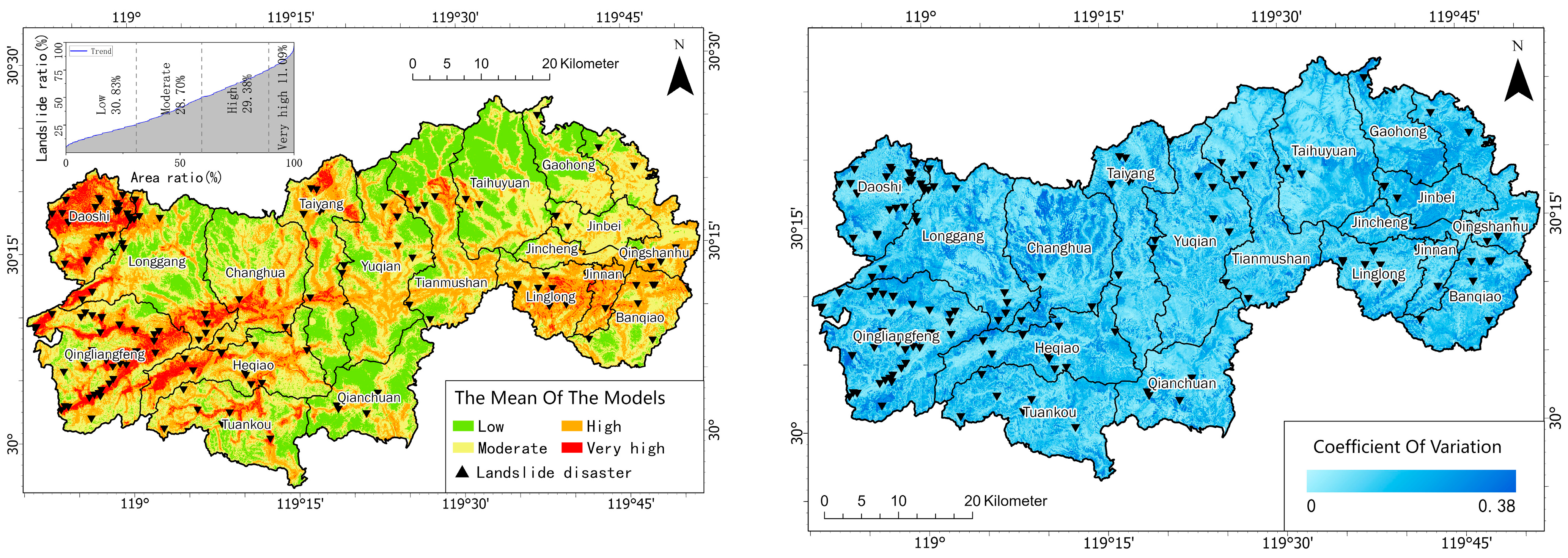
At pixel level, all four models consistently predicted that the very high landslide susceptibility is mostly distributed in the western and southeastern regions (Figure 5), while the other regions generally had low risk. Compared with the three decision-tree-based models, MLP predicted more “very high” risk pixels in the two regions. Considering the uncertainties from the different methods, we further calculated the mean landslide susceptibility and CV (Figure 6). The results also indicated that the southeastern and western regions had the highest landslide risks, and these regions generally had the lowest CV, further implying high agreements and confidence for the high landslide susceptibility predictions. These high risk areas generally have very different LCFs (Figure 2), implying different controlling LCFs for landslide susceptibility. At town scale, the “very-high” risk areas are mostly located in Daoshi and Jinnan, southeastern Qingliangfeng, Longgang, Changhua and Linglong, eastern Heqiao, and northern Banqiao Towns (Figure 6).

3.4. Driving Mechanisms of Landslide Suceptibility

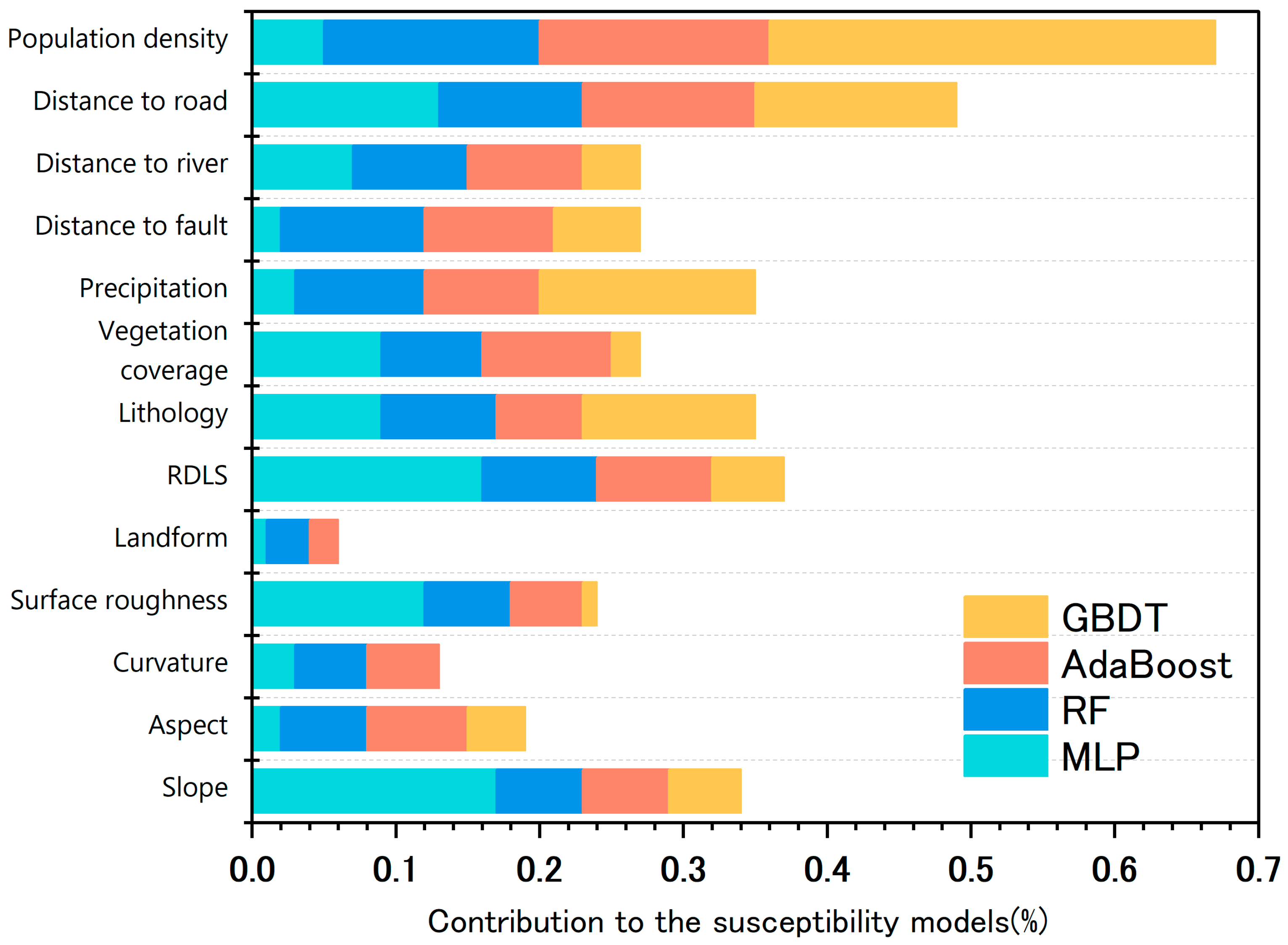
The spatial distribution patterns of landslide susceptibility can be attributable to the spatial characteristics of LCFs (Figure 2). The comparison of relative importance of LCFs is essential to improve the efficiency and the performance of landslide prediction models, and provide implications to policy-makers. In this study, the Gini information gain method was selected to determine the relative importance of each controlling factor. Different models indicated varied major contributing factors (Figure 7). For the RF model, the most important contributor is population density (15%), followed by distance to road (10%). For the MLP model, the most important contributors are slope (17%), relief amplitude (16%) and distance to road (13%). For the AdaBoost model, the major contributing factors are population density (16%) and distance to road (12%). For the GBDT model, the major contributing factors are population density (31%), precipitation (15%) and distance to road (12%). In the thirteen LCFs, RF, AdaBoost and GBDT models agreed well that population density has the largest relative importance. Landform and curvature generally had the minimum relative importance, indicating these two factors had less effect in data fitting and classification. Overall, population density, distance to road, and relief amplitude are generally among the top three major contributing factors for all four models. At town level, our results indicated that the leading contributing LCFs varied significantly. For Daoshi Town, the top three LCFs were population density, distance to fault, and curvature; for Jinnan, the top three LCFs were population density, relief amplitude, and aspect; for Linglong, the top three LCFs were aspect, relief amplitude, and population density; for Qingliangfeng, the top three LCFs were population density, precipitation, and distance to fault. Generally, population density, relief amplitude, and distance to fault were the most important LCFs for the high-risk towns.

4. Discussion

4.1. Effectiveness for Different Models

Compared with traditional landslide susceptibility prediction methods, the use of machine learning algorithms greatly improves the prediction accuracy [26]. How to choose and use these algorithms, however, is still debatable for researchers. Based on multiple evaluation metrics, our study found that all four models can adequately predict landslide susceptibility in the study region. Among these models, the RF model performed the best, followed by AdaBoost and GBDT, all having significantly higher F1-score and AUC values than the MLP model. In many previous studies for model comparisons, various conclusions were drawn. For example, Youssef and Pourghasemi [31] indicated that the RF model produced the best performance as compared with other machine learning methods including SVM. They argued that landslide susceptibility models depend on the variables used to implement the models, and thus RF performed better in some specific areas, while yielded poorer results in some other areas. Hong et al. [21] also concluded that the LR method has better performance than RF in terms of AUC in assessing landslide susceptibility in Lianhua County, China. The study by Tien Bui et al. [33] indicated that the MLP method outperformed several other traditional ML models. Pourghasemi and Rahmati [4] applied 10 machine learning techniques for landslide susceptibility assessment and compared their performance. The results indicated that the frequency ratio method had the best performance compared to RF and other models in terms of AUC values.
In recent years, the ensemble methods, which combine multiple classifiers for making decisions, are increasingly applied to predict landslide susceptibility. Many previous comparative studies showed that ensemble-based machine learning methods are superior to single machine learning methods in accuracy and robustness, which can increase the availability of high-resolution LSM [28,74]. Chen et al. [20] reported that the GBDT method outperformed the other machine learning methods, and was able to provide strong technical support for producing landslide susceptibility maps in the Three Gorges Reservoir area. Kadavi et al. [29] also concluded that ensemble models have higher accuracy than traditional frequency ratio models in Sacheon-myeon. However, in this study, we also applied both regular single classifier (MLP and RF) and ensemble classifiers (GBDT and AdaBoost), and we found that the RF method performed slightly better than the GBDT and AdaBoost methods, but the MLP method performed less accurately than other methods. Sahin [75] produced a landslide susceptibility map using three decision-tree-based ensemble methods, including GBDT, XGB, and RF, and his study also indicated that the RF method had a slightly lower prediction error and higher accuracy than GBDT. Overall, the performance of machine learning models depends on the data used, and implicitly on the extent of the study areas [3].
Except for the ensemble method, another increasingly trend is to apply various integration or stacking algorithms to landslide susceptibility prediction. It can integrate different types of models, thereby reducing errors that cannot be eliminated by a single model and greatly improving the prediction accuracy [14,70,76,77]. For example, Chen et al. [18,45] integrated RF with the bivariate statistical index (SI) and other machine learning methods to assess landslide susceptibility in China and proved the integrated method performed better. Huan et al. [27] integrated RF with LP, GBDT, and XGB to predict landslides in Hunan Province, China. In the near future, these integrated methods could be the most popular and effective methods to predict landslide susceptibility.

4.2. Major Contributing Factors

Identifying the contribution from LCFs can help better understand the reasons for the occurrence of landslides in a region, and thus provide implications for policy-makers [33]. Owing to the characteristics of the decision-tree algorithm, it can directly use Gini impurity to calculate the contribution of each factor to the model prediction [78]. The factor contributions of MLP were calculated by using the difference between the F1-score on the training set obtained by removing a certain factor and the original overall accuracy. Our results showed that the LCFs have different contributions to landslide susceptibility in different models. The factors that contribute most to the four models were population density, relief amplitude, and distance to road, respectively. Our results are partially in line with many previous studies performed at various spatial scales. For example, Saha et al. [79] indicated that elevation, distance from road, and precipitation are the most important features. Kawabata and Bandibas [80] found that geological factors were the most important factors in landslide occurrence. Liao et al. [39] concluded that elevation, lithology, distance from faults, and average annual rainfall were the most significant contributing factors in Wushan and Wuxi, Chongqing, China, while vegetation coverage (NDVI) and land cover had no significant contributions. Youssef et al. [81] reported that slope angle, land use, and elevation have higher importance in landslide occurrence. Meinhardt et al. [82] reported that lithology, slope gradient, and precipitation increase have higher importance. Pourghasemi and Rahmati [4] indicated that six LCFs including slope angle, distance from road, slope length, distance from fault, drainage density, and altitude were the major factors in predicting landslide susceptibility according to their generalized additive model (GAM) analysis. Therefore, different study areas or model algorithms lead to significant differences in the major contributing LCFs [3,4].
To further identify the contributions of the three leading LCFs, we applied the Jenks natural breaks and quantile methods to further divide the three factors into four classes (Table 8). The frequency ratio (FR) and information quality (I) for each class were used to estimate the existing relation between the three variables and the presence of landslides [17,44]. The results showed 81% of the landslide hazards occurred in areas with low population density (≤2 persons/km2). For distance to road, the information quality and FR were the highest when the distance was less than 391.6 m. For relief amplitude (RDLS), the unit height difference between 87 and 156 m was the most vulnerable area, in which the FR and information quality were 0.52 and 0.18, respectively. In summary, the construction of roads could greatly destroy the geological conditions. Therefore, the highest risk was generally closer to the road.

4.3. Implications for Policymaking and Disaster Mitigation

Landslides pose great threats to the environment and socioeconomic development. LSM can show the users and stakeholders risk levels and where landslides are expected, contributing to adopt policies and to take proactive action to reduce or avoid landslides and their negative consequences [83]. Users and stakeholders may include policy-makers; government administrations; land use planners; real estate agents; environmental agencies; road, transport and utility companies; agriculture and forest managers; insurance companies; and citizens. Our findings indicate that the results from the four models can help decision-makers identify the vulnerable areas in the Lin’An District. We identified the high-risk areas, which are mostly distributed in the western and southeastern regions, including most areas in Daoshi, Jinnan, Linglong, and Qingliangfeng towns, so the related stakeholders can make decisions to avoid these high-risk areas for cropland, residential zones, roads, and utility and infrastructure construction. The mitigation can include structural and geotechnical measures, and political, legal, and administrative measures to protect endangered populations and the environment in these vulnerable areas [83].
In addition, we found that the leading contributing factors to landslide susceptibility varied significantly among towns. Therefore, our study can provide guidance on specific and different mitigation measures to the stakeholders in different towns. For example, Daoshi Town has the highest landslide risk and the major contributing factors are population density, distance to fault, and curvature. Daoshi has the highest average elevation and more than 90% of the land area is covered by low and middle mountain landforms, so the stakeholders should try to avoid the construction of residential areas in the higher mountain areas and areas with less hard bedrock. In addition, this geographical environment also leads to low local population density (2 person per km2 on average), and most residents should be concentrated in the flat valley areas. Therefore, relevant units should focus on monitoring the mountain conditions around the valley to avoid large-scale landslide disasters in these populated areas. In contrast, the major contributing factors are population density, precipitation, and distance to fault in Jinnan Town, where the major landform is plain and two fault lines pass beneath this town (Figure 2c). Therefore, the specific mitigation measures should not give attention to elevation, and land use planning should focus on drainage facilities to avoid building residential facilities in areas with active geological movement. These same leading contributing factors apply to Jinnan and Qingliangfeng Towns; however, the major landforms in Qingliangfeng are low and middle mountains (Figure 2c). Therefore, land use planning should give more attention to avoiding areas with both high precipitation and slopes.
In recent years, applications of landslide susceptibility models and the susceptibility maps in landslide early-warning systems have emerged at different spatial scales. For example, Hong and Adler [84] developed a global early-warning system for rainfall and seismically triggered landslides based on a global-scale susceptibility model. In the future, we can integrate the best models, remote sensing data, and inventory data to develop an early-warning system for the Lin’An District.

5. Conclusions

Machine learning methods have been widely applied in LSM during the recent several years and their good performance has been proved for worldwide regions and countries, but there is no consensus on the best methods and leading contributing factors for specific regions. Therefore, it is often necessary to identify the best methods and contributing factors in specific regions in LSM. To find the best prediction methods and provide spatial assessments of landslide susceptibility in the landslide-vulnerable Lin’An District, this research applied two single-classifier-based (MLP and RF) and two ensemble-based (AdaBoost and GBDT) machine learning methods to predict LSM. The comparisons and evaluations indicated that all models can be adequately applied to produce landslide susceptibility maps at 30 m spatial scale for the study area, with the better performance from the RF, AdaBoost and GBDT models in terms of both F1-score and AUC values. The three decision-tree models (RF, AdaBoost, and GBDT) matched better than the MLP in predicting the distribution of landslide susceptibility, especially for the high-risk areas. The importance and contributions from the screened 13 LCFs were further identified based on these models, and the results revealed that different factors have different importance in the four models, implying the selection of LCFs is important for LSM. The leading contributing factors for the entire study region are population density, distance to fault, and relief amplitude, while the four high-risk towns identified have slightly different leading factors. Our study is the first report concerning landslide susceptibility specifically for the study region at both pixel (30 m) and town scales. Therefore, our identified methods, the predicted LSM, and the identified leading contributing factors can help produce a crucial guide for general planning and assessment purposes in the study region, thus enabling proactive actions to reduce or avoid landslides and their damage. Our findings further suggest that protection and mitigation measures should be unique for different areas and towns.

Author Contributions

Conceptualization: H.Y., W.P. and J.Z.; methodology: H.Y., W.P. and G.C.; validation: H.Y. and J.Z.; formal analysis: H.Y., W.P. and J.Z.; data curation: W.P.; writing—original draft: H.Y., W.P., J.Z. and G.C.; writing—review and editing: G.C., H.Y., W.P. and J.Z.; visualization: W.P. and H.Y.; supervision: G.C.; project administration: G.C.; funding acquisition: G.C. All authors have read and agreed to the published version of the manuscript.

Funding

This work was funded by the Natural Science Foundation of Zhejiang Province (grant number LY20C030001), the Scientific Research Foundation of Zhejiang A&F University (grant number 2034020080), and the Overseas Expertise Introduction Project for Discipline Innovation (111 Project; grant number D18008).

Data Availability Statement

The data that support the findings of this study are available on request from the authors ([email protected]).

Conflicts of Interest

The authors declare no conflict of interest.

References

  1. Fall, M.; Azzam, R.; Noubactep, C. A multi-method approach to study the stability of natural slopes and landslide susceptibility mapping. Eng. Geol. 2006, 82, 241–263. [Google Scholar] [CrossRef]
  2. Feizizadeh, B.; Blaschke, T. An uncertainty and sensitivity analysis approach for GIS-based multicriteria landslide susceptibility mapping. Int. J. Geogr. Inf. Sci. 2014, 28, 610–638. [Google Scholar] [CrossRef] [PubMed] [Green Version]
  3. Reichenbach, P.; Rossi, M.; Malamud, B.D.; Mihir, M.; Guzzetti, F. A review of statistically-based landslide susceptibility models. Earth Sci. Rev. 2018, 180, 60–91. [Google Scholar] [CrossRef]
  4. Pourghasemi, H.R.; Rahmati, O. Prediction of the landslide susceptibility: Which algorithm, which precision? Catena 2018, 162, 177–192. [Google Scholar] [CrossRef]
  5. Ma, Z.; Mei, G. Deep learning for geological hazards analysis: Data, models, applications, and opportunities. Earth Sci. Rev. 2021, 223, 103858. [Google Scholar] [CrossRef]
  6. Felicísimo, A.; Cuartero, A.; Remondo, J.; Quirós, E. Mapping landslide susceptibility with logistic regression, multiple adaptive regression splines, classification and regression trees, and maximum entropy methods: A comparative study. Landslides 2013, 10, 175–189. [Google Scholar] [CrossRef]
  7. Chen, W.; Pourghasemi, H.R.; Kornejady, A.; Zhang, N. Landslide spatial modeling: Introducing new ensembles of ANN, MaxEnt, and SVM machine learning techniques. Geoderma 2017, 305, 314–327. [Google Scholar] [CrossRef]
  8. Huang, Y.; Zhao, L. Review on landslide susceptibility mapping using support vector machines. Catena 2018, 165, 520–529. [Google Scholar] [CrossRef]
  9. Sharifi, A. Flood mapping using relevance vector machine and SAR data: A case study from Aqqala, Iran. J. Indian Soc. Remote Sens. 2020, 48, 1289–1296. [Google Scholar] [CrossRef]
  10. Sharifi, A.; Hosseingholizadeh, M. The effect of rapid population growth on urban expansion and destruction of green space in Tehran from 1972 to 2017. J. Indian Soc. Remote Sens. 2019, 47, 1063–1071. [Google Scholar] [CrossRef]
  11. Jalayer, S.; Sharifi, A.; Abbasi-Moghadam, D.; Tariq, A.; Qin, S. Modeling and predicting land use land cover spatiotemporal changes: A case study in chalus watershed, Iran. IEEE J. Sel. Top. Appl. Earth Obs. Remote Sens. 2022, 15, 5496–5513. [Google Scholar] [CrossRef]
  12. Raghu, S.; Sriraam, N. Optimal configuration of multilayer perceptron neural network classifier for recognition of intracranial epileptic seizures. Expert Syst. Appl. 2017, 89, 205–221. [Google Scholar] [CrossRef]
  13. Zare, M.; Pourghasemi, H.R.; Vafakhah, M.; Pradhan, B. Landslide susceptibility mapping at vaz watershed (Iran) using an artificial neural network model: A comparison between multilayer perceptron (MLP) and radial basic function (RBF) algorithms. Arab. J. Geosci. 2013, 6, 2873–2888. [Google Scholar] [CrossRef]
  14. Binh Thai, P.; Dieu Tien, B.; Prakash, I.; Dholakia, M.B. Hybrid integration of multilayer perceptron neural networks and machine learning ensembles for landslide susceptibility assessment at himalayan area (India) using GIS. Catena 2017, 149, 52–63. [Google Scholar]
  15. Moayedi, H.; Mehrabi, M.; Mosallanezhad, M.; Rashid, A.S.A.; Pradhan, B. Modification of landslide susceptibility mapping using optimized pso-ann technique. Eng. Comput. 2019, 35, 967–984. [Google Scholar] [CrossRef]
  16. Kalantar, B.; Pradhan, B.; Naghibi, S.A.; Motevalli, A.; Mansor, S. Assessment of the effects of training data selection on the landslide susceptibility mapping: A comparison between support vector machine (SVM), logistic regression (LR) and artificial neural networks (ANN). Geomat. Nat. Hazards Risk 2018, 9, 49–69. [Google Scholar] [CrossRef]
  17. Wu, Y.; Ke, Y.; Chen, Z.; Liang, S.; Zhao, H.; Hong, H. Application of alternating decision tree with adaboost and bagging ensembles for landslide susceptibility mapping. Catena 2020, 187, 104396. [Google Scholar] [CrossRef]
  18. Chen, W.; Li, Y. GIS-based evaluation of landslide susceptibility using hybrid computational intelligence models. Catena 2020, 195, 104777. [Google Scholar] [CrossRef]
  19. Song, J.; Wang, Y.; Fang, Z.; Peng, L.; Hong, H. Potential of ensemble learning to improve tree-based classifiers for landslide susceptibility mapping. IEEE J. Sel. Top. Appl. Earth Obs. Remote Sens. 2020, 13, 4642–4662. [Google Scholar] [CrossRef]
  20. Chen, T.; Zhu, L.; Niu, R.; Trinder, C.J.; Peng, L.; Lei, T. Mapping landslide susceptibility at the three gorges reservoir, China, using gradient boosting decision tree, random forest and information value models. J. Mt. Sci. 2020, 17, 670–685. [Google Scholar] [CrossRef]
  21. Hong, H.; Pourghasemi, H.R.; Pourtaghi, Z.S. Landslide susceptibility assessment in Lianhua county (China): A comparison between a random forest data mining technique and bivariate and multivariate statistical models. Geomorphology 2016, 259, 105–118. [Google Scholar] [CrossRef]
  22. Sun, D.; Wen, H.; Wang, D.; Xu, J. A random forest model of landslide susceptibility mapping based on hyperparameter optimization using bayes algorithm. Geomorphology 2020, 362, 107201. [Google Scholar] [CrossRef]
  23. Kim, J.-C.; Lee, S.; Jung, H.-S.; Lee, S. Landslide susceptibility mapping using random forest and boosted tree models in Pyeong-chang, Korea. Geocarto Int. 2018, 33, 1000–1015. [Google Scholar] [CrossRef]
  24. Viet-Ha, N.; Shirzadi, A.; Shahabi, H.; Chen, W.; Clague, J.J.; Geertsema, M.; Jaafari, A.; Avand, M.; Miraki, S.; Asl, D.T.; et al. Shallow landslide susceptibility mapping by random forest base classifier and its ensembles in a semi-arid region of Iran. Forests 2020, 11, 421. [Google Scholar]
  25. Trigila, A.; Iadanza, C.; Esposito, C.; Scarascia-Mugnozza, G. Comparison of logistic regression and random forests techniques for shallow landslide susceptibility assessment in Giampilieri (NE Sicily, Italy). Geomorphology 2015, 249, 119–136. [Google Scholar] [CrossRef]
  26. Akgun, A. A comparison of landslide susceptibility maps produced by logistic regression, multi-criteria decision, and likelihood ratio methods: A case study at Izmir, Turkey. Landslides 2012, 9, 93–106. [Google Scholar] [CrossRef]
  27. Huan, Y.; Song, L.; Khan, U.; Zhang, B. Stacking ensemble of machine learning methods for landslide susceptibility mapping in Zhangjiajie City, Hunan Province. Environ. Earth Sci. 2023, 82, 35. [Google Scholar] [CrossRef]
  28. Hong, H.; Liu, J.; Bui, D.T.; Pradhan, B.; Acharya, T.D.; Pham, B.T.; Zhu, A.X.; Chen, W.; Ahmad, B.B. Landslide susceptibility mapping using j48 decision tree with adaboost, bagging and rotation forest ensembles in the Guangchang area (China). Catena 2018, 163, 399–413. [Google Scholar] [CrossRef]
  29. Kadavi, P.R.; Lee, C.W.; Lee, S. Application of ensemble-based machine learning models to landslide susceptibility mapping. Remote Sens. 2018, 10, 1252. [Google Scholar] [CrossRef] [Green Version]
  30. Rodriguez, J.J.; Kuncheva, L.I.; Alonso, C.J. Rotation forest: A new classifier ensemble method. IEEE Trans. Pattern Anal. Mach. Intell. 2006, 28, 1619–1630. [Google Scholar] [CrossRef] [PubMed]
  31. Youssef, A.M.; Pourghasemi, H.R. Landslide susceptibility mapping using machine learning algorithms and comparison of their performance at Abha Basin, Asir Region, Saudi Arabia. Geosci. Front. 2021, 12, 639–655. [Google Scholar] [CrossRef]
  32. Ng, C.W.W.; Yang, B.; Liu, Z.Q.; Kwan, J.S.H.; Chen, L. Spatiotemporal modelling of rainfall-induced landslides using machine learning. Landslides 2021, 18, 2499–2514. [Google Scholar] [CrossRef]
  33. Tien Bui, D.; Tuan, T.A.; Klempe, H.; Pradhan, B.; Revhaug, I. Spatial prediction models for shallow landslide hazards: A comparative assessment of the efficacy of support vector machines, artificial neural networks, kernel logistic regression, and logistic model tree. Landslides 2016, 13, 361–378. [Google Scholar] [CrossRef]
  34. Carrara, A.; Pike, R.J. GIS technology and models for assessing landslide hazard and risk. Geomorphology 2008, 94, 57–260. [Google Scholar] [CrossRef]
  35. Jebur, M.N.; Pradhan, B.; Tehrany, M.S. Optimization of landslide conditioning factors using very high-resolution airborne laser scanning (LiDAR) data at catchment scale. Remote Sens. Environ. 2014, 152, 150–165. [Google Scholar] [CrossRef]
  36. Borgomeo, E.; Hebditch, K.V.; Whittaker, A.C.; Lonergan, L. Characterising the spatial distribution, frequency and geomorphic controls on landslide occurrence, molise, italy. Geomorphology 2014, 226, 148–161. [Google Scholar] [CrossRef]
  37. Gibson, A.D.; Culshaw, M.G.; Dashwood, C.; Pennington, C.V.L. Landslide man-agement in the UK—The problem of managing hazards in a ‘low-risk’ environment. Landslides 2013, 10, 599–610. [Google Scholar] [CrossRef] [Green Version]
  38. Lin, L.; Chen, G.; Shi, W.; Jin, J.; Wu, J.; Huang, F.; Chong, Y.; Meng, Y.; Li, Y.; Zhang, Y. Spatiotemporal evolution pattern and driving mechanisms of landslides in the wenchuan earthquake-affected region: A case study in the Bailong river basin, China. Remote Sens. 2022, 14, 2339. [Google Scholar] [CrossRef]
  39. Liao, M.; Wen, H.; Yang, L. Identifying the essential conditioning factors of landslide susceptibility models under different grid resolutions using hybrid machine learning: A case of Wushan and Wuxi counties, China. Catena 2022, 217, 106428. [Google Scholar] [CrossRef]
  40. Lin, Q.; Lima, P.; Steger, S.; Glade, T.; Jiang, T.; Zhang, J.; Liu, T.; Wang, Y. National-scale data-driven rainfall induced landslide susceptibility mapping for China by accounting for incomplete landslide data. Geosci. Front. 2021, 12, 101248. [Google Scholar] [CrossRef]
  41. Aleotti, P.; Chowdhury, R. Landslide hazard assessment: Summary review and new perspectives. Bull. Eng. Geol. Environ. 1999, 58, 21–44. [Google Scholar] [CrossRef]
  42. Huang, R. Large-scale landslides and their sliding mechanisms in China since the 20th century. Chin. J. Rock Mech. Eng. 2007, 3, 433–454. [Google Scholar]
  43. Hu, R.; Fan, L.; Wang, S.; Wang, L.; Wang, X. Theory and method for landslide risk assessment-current status and future development. J. Eng. Geol. 2013, 21, 76–84. [Google Scholar]
  44. Bui, D.T.; Tsangaratos, P.; Nguyen, V.T.; Liem, N.V.; Trinh, P.T. Comparing the prediction performance of a deep learning neural network model with conventional machine learning models in landslide susceptibility assessment. Catena 2020, 188, 104426. [Google Scholar] [CrossRef]
  45. Chen, W.; Xie, X.; Peng, J.; Shahabi, H.; Hong, H. GIS-based landslide susceptibility evaluation using a novel hybrid integration approach of bivariate statistical based random forest method. Catena 2018, 164, 135–149. [Google Scholar] [CrossRef]
  46. Wu, W.; Sidle, R.C. A distributed slope stability model for steep forested basins. Water Resour. Res. 1995, 31, 2097–2110. [Google Scholar] [CrossRef]
  47. Bao, Q.; Zhang, Y.; Wang, Y.; Wang, Y. Analysis on the relationships between the small range debris flow and rainfall in Linan, Zhejiang Province. Bull. Sci. Technol. 2012, 28, 44–50. [Google Scholar]
  48. Li, L.; Lan, H.; Guo, C.; Zhang, Y.; Li, Q.; Wu, Y. Geohazard susceptibility assessment along the sichuan-tibet railway and its adjacent area using an improved frequency ratio method. Geoscience 2017, 31, 911–929. [Google Scholar]
  49. Lan, H.; Wu, F.; Zhou, C.; Wang, S. Analysis on susceptibility of GIS based landslide triggering factors in Yunnan Xiaojiang watershed. Chin. J. Rock Mech. Eng. 2002, 21, 1500–1506. [Google Scholar]
  50. Li, B.; Pan, B.; Han, J. Basic terrestrial geomorphological types in China and thier circumscriptions. Quat. Sci. 2008, 28, 535–543. [Google Scholar]
  51. Zhang, H.; Wang, X.; Yu, Z. Slope surface complexity factor extract and analysis based on ArcGIS. J. Cent. China Norm. Univ. (Nat. Sci.) 2009, 43, 323–326. [Google Scholar]
  52. Tu, H.; Liu, Z. Demonstrating on optimum statistica unit of relief amplitude in China. J. Hubei Univ. 1990, 12, 266–271. [Google Scholar]
  53. Zevenbergen, L.W.; Thorne, C.R. Quantitative analysis of land surface topography. Earth Surf. Process. Landf. 1987, 12, 47–56. [Google Scholar] [CrossRef]
  54. Hair, J.F.; Black, W.C.; Babin, B.J.; Anderson, R.E. Multivariate Data Analysis: A Global Perspective; Pearson: Delhi, India, 2014. [Google Scholar]
  55. Hembram, T.k.; Paul, G.C.; Saha, S. Spatial prediction of susceptibility to gully erosion in Jainti River Basin, Eastern India: A comparison of information value and logistic regression models. Model. Earth Syst. Environ. 2019, 5, 689–708. [Google Scholar] [CrossRef]
  56. Saha, S.; Gayen, A.; Pourghasemi, H.R.; Tiefenbacher, J.P. Identification of soil erosion-susceptible areas using fuzzy logic and analytical hierarchy process modeling in an agricultural watershed of Burdwan district, India. Environ. Earth Sci. 2019, 78, 649. [Google Scholar] [CrossRef]
  57. Wang, Y.; Fang, Z.C.; Hong, H.Y. Comparison of convolutional neural networks for landslide susceptibility mapping in Yanshan county, China. Sci. Total Environ. 2019, 666, 975–993. [Google Scholar] [CrossRef]
  58. Freund, Y.; Schapire, R.E. A decision-theoretic generalization of on-line learning and an application to boosting. J. Comput. Syst. Sci. 1997, 55, 119–139. [Google Scholar] [CrossRef] [Green Version]
  59. Schapire, R.E. The strength of weak learnability. Mach. Learn. 1990, 5, 197–227. [Google Scholar] [CrossRef] [Green Version]
  60. Freund, Y.; Schapire, R.E. A short introduction to boosting. J. Jpn. Soc. Artif. Intell. 1999, 14, 771–780. [Google Scholar]
  61. Friedman, J.H.; Hastie, T.; Tibshirani, R. Additive logistic regression: A statistical view of boosting. Ann. Stat. 2000, 28, 337–407. [Google Scholar] [CrossRef]
  62. Friedman, J.H. Stochastic gradient boosting: Nonlinear methods and data mining. Comput. Stat. Data Anal. 2002, 38, 367–378. [Google Scholar]
  63. Liang, Z.; Wang, C.; Duan, Z.; Liu, H.; Khan, K.J. A hybrid model consisting of supervised and unsupervised learning for landslide susceptibility mapping. Remote Sens. 2021, 13, 1464. [Google Scholar] [CrossRef]
  64. Ghritlahre, H.K.; Prasad, R.K. Exergetic performance prediction of solar air heater using mlp, grnn and rbf models of artificial neural network technique. J. Environ. Manag. 2018, 223, 566–575. [Google Scholar] [CrossRef]
  65. LeCun, Y.; Bengio, Y.; Hinton, G. Deep learning. Nature 2015, 521, 436–444. [Google Scholar] [CrossRef] [PubMed]
  66. Rumelhart, D.E.; Hinton, G.E.; Williams, R.J. Learning representations by back-propagation errors. Nature 1986, 323, 533–536. [Google Scholar] [CrossRef]
  67. Efron, B.; Tibshirani, R.J. An Introduction to the Bootstrap; Chapman and Hall/CRC: New York, NY, USA, 1994. [Google Scholar]
  68. Krstajic, D.; Buturovic, L.J.; Leahy, D.E.; Thomas, S. Cross-validation pitfalls when selecting and assessing regression and classification models. J. Cheminform. 2014, 6, 10. [Google Scholar] [CrossRef] [PubMed] [Green Version]
  69. Bergstra, J.; Bengio, Y. Random search for hyper-parameter optimization. J. Mach. Learn. Res. 2012, 13, 281–305. [Google Scholar]
  70. Kardani, N.; Zhou, A.; Nazem, M.; Shen, S. Improved prediction of slope stability using a hybrid stacking ensemble method based on finite element analysis and field data. J. Rock Mech. Geotech. Eng. 2021, 13, 188–201. [Google Scholar] [CrossRef]
  71. Chen, M.; Wu, J.; Liu, L.; Zhao, W.; Tian, F.; Shen, Q.; Zhao, B.; Du, R. DR-Net: An improved network for building extraction from high resolution remote sensing image. Remote Sens. 2021, 13, 294. [Google Scholar]
  72. Roy, J.; Saha, S.; Arabameri, A.; Blaschke, T.; Bui, D.T. A novel ensemble approach for landslide susceptibility mapping (LSM) in Darjeeling and Kalimpong districts, West Bengal, India. Remote Sens. 2019, 11, 2866. [Google Scholar] [CrossRef] [Green Version]
  73. Hanley, J.A.; McNeil, B.J. The meaning and use of the area under a receiver operating characteristic (ROC) curve. Radiology 1982, 143, 29–36. [Google Scholar] [CrossRef] [PubMed] [Green Version]
  74. Merghadi, A.; Yunus, A.P.; Dou, J.; Whiteley, J.; ThaiPham, B.; Bui, D.T. Machine learning methods for landslide susceptibility studies: A comparative overview of algorithm performance. Earth Sci. Rev. 2020, 207, 103225. [Google Scholar] [CrossRef]
  75. Sahin, E.K. Assessing the predictive capability of ensemble tree methods for landslide susceptibility mapping using XGBoost, gradient boosting machine, and random forest. SN Appl. Sci. 2020, 2, 1308. [Google Scholar] [CrossRef]
  76. Binh Thai, P.; Prakash, I.; Singh, S.K.; Shirzadi, A.; Shahabi, H.; Thi-Thu-Trang, T.; Dieu Tien, B. Landslide susceptibility modeling using reduced error pruning trees and different ensemble techniques: Hybrid machine learning approaches. Catena 2019, 175, 203–218. [Google Scholar]
  77. Abedini, M.; Ghasemian, B.; Shirzadi, A.; Shahabi, H.; Chapi, K.; Binh Thai, P.; Bin Ahmad, B.; Dieu Tien, B. A novel hybrid approach of bayesian logistic regression and its ensembles for landslide susceptibility assessment. Geocarto Int. 2019, 34, 1427–1457. [Google Scholar] [CrossRef]
  78. Goetz, J.N.; Brenning, A.; Petschko, H.; Leopold, P. Evaluating machine learning and statistical prediction techniques for landslide susceptibility modeling. Comput. Geosci. 2015, 81, 1–11. [Google Scholar] [CrossRef]
  79. Saha, S.; Arabameri, A.; Saha, A.; Blaschke, T.; Ngo, P.T.T.; Viet Ha, N.; Band, S.S. Prediction of landslide susceptibility in Rudraprayag, India using novel ensemble of conditional probability and boosted regression tree-based on cross-validation method. Sci. Total Environ. 2021, 764, 142928. [Google Scholar] [CrossRef] [PubMed]
  80. Kawabata, D.; Bandibas, J. Landslide susceptibility mapping using geological data, a dem from aster images and an artificial neural network (ANN). Geomorphology 2009, 113, 97–109. [Google Scholar] [CrossRef]
  81. Youssef, A.M.; Pourghasemi, H.R.; Pourtaghi, Z.S.; Al-Katheeri, M.M. Landslide susceptibility mapping using random forest, boosted regression tree, classification and regression tree, and general linear models and comparison of their performance at Wadi Tayyah Basin, Asir Region, Saudi Arabia. Landslides 2016, 13, 839–856. [Google Scholar]
  82. Meinhardt, M.; Fink, M.; Tünschel, H. Landslide susceptibility analysis in central Vietnam based on an incomplete landslide inventory: Comparison of a new method to calculate weighting factors by means of bivariate statistics. Geomorphology 2015, 234, 80–97. [Google Scholar] [CrossRef]
  83. Turner, A.K. Social and environmental impacts of landslides. Innov. Infrastruct. Solut. 2018, 3, 70. [Google Scholar] [CrossRef]
  84. Hong, Y.; Adler, R.F. Towards an early warning system for global landslides triggered by rainfall and earthquake. Int. J. Remote Sens. 2007, 28, 3713–3719. [Google Scholar] [CrossRef]
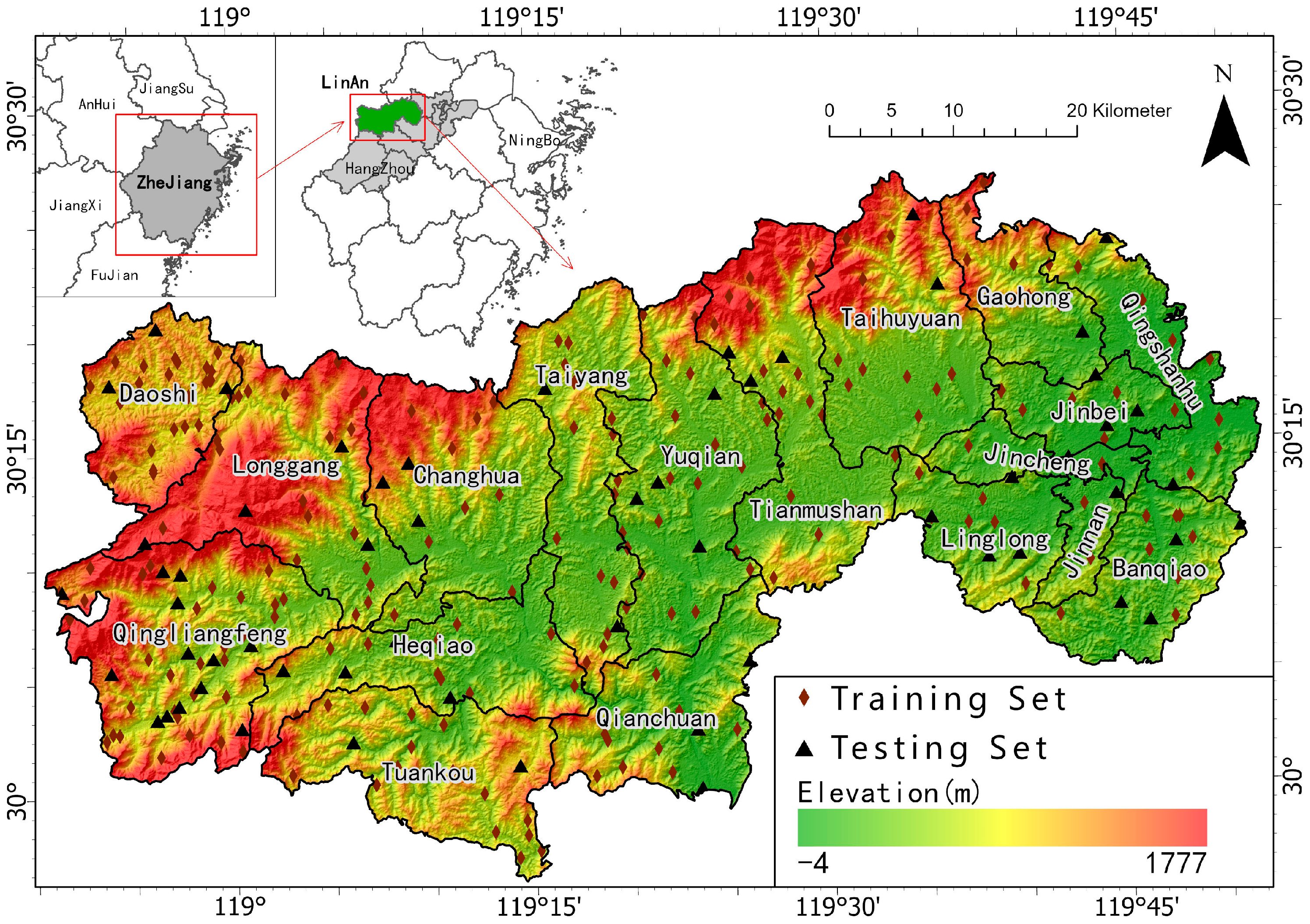
Figure 1. Location, elevation (m), towns, and landslide sample points in the study region. Note: type 0: sample points without landslide; type 1: sample points with landslide.
Remotesensing 15 01886 g001
Figure 2. The spatial patterns of some landslide conditioning factors. (a): surface roughness; (b): lithology and fault lines; (c): landforms and rivers; (d): population density (persons/km2) and road; (e): curvature; (f): precipitation (mm); (g): vegetation coverage; (h): slope; (i): aspect; (j): relief amplitude.
Remotesensing 15 01886 g002
Figure 3. The research work flow. AdaBoost: adaptive boosting; GBDT: gradient-boosting decision tree; MLP: multilayer perceptron; RF: random forest.
Remotesensing 15 01886 g003
Figure 4. Area under the curve (AUC) values for the receiver–operating characteristic (ROC) curves for the four models.
Remotesensing 15 01886 g004
Figure 5. Landslide susceptibility maps predicted by the RF, MLP, AdaBoost, and GBDT machine learning methods.
Remotesensing 15 01886 g005
Figure 6. The mean landslide susceptibility levels (left) predicted by the four models and the coefficient of variance (CV; right). Note: The black triangles are the inventory landslide points; the polygons are town boundaries.
Remotesensing 15 01886 g006
Figure 7. Relative importance of conditioning factors in the four models.
Remotesensing 15 01886 g007
Table 1. Data sources, format and other characteristics.
Data NameFormatSpatial ResolutionAcquisition DateSource
DEMRaster30 m-https://www.gscloud.cn (accessed on 1 March 2023)
Geological conditionShapefile--https://www.resdc.cn (accessed on 1 March 2023)
Road networkShapefile--https://www.resdc.cn (accessed on 1 March 2023)
Land coverRaster10 m2020https://livingatlas.arcgis.com/landcover (accessed on 1 March 2023)
Population densityRaster30 m2020https://www.worldpop.org (accessed on 1 March 2023)
Sentinel-2A imagesRaster10 m5 March 2020–11 March 2020https://scihub.copernicus.eu (accessed on 1 March 2023)
Landslide plotsShapefile-1945–2020https://www.resdc.cn (accessed on 1 March 2023)
Mean precipitation in the monsoon seasonRaster1 km2010–2018https://www.worldclim.org (accessed on 1 March 2023)
Water system mapShapefile-2022https://www.resdc.cn (accessed on 1 March 2023)
Table 2. The optimized hyperparameter values for the selected four models.
ModelsHyperparameter Values
AdaBoostNumber of trees = 40, learning rate = 1
GBDTNumber of trees = 17, learning rate = 0.1
MLPLearning rate = 0.005, decay = 0.01, epoch = 300, batch size = 16
RFNumber of trees = 17, min samples leaf = 3, max features = 3
Table 3. Multicollinearity diagnosis for the 13 landslide condition factors (LCFs).
LCFsVIFTolerance
slope1.93950.5156
aspect1.12750.8869
curvature1.02630.9743
surface roughness2.09800.4766
landform4.98200.2007
RDLS2.58170.3873
lithology1.19640.8359
vegetation coverage1.47450.6782
precipitation4.42800.2258
distance to fault1.16020.8619
distance to river1.34370.7442
distance to road1.28610.7776
population density2.13210.4690
Table 4. Accuracy assessment results for the LR, SVM, MLP, and RF models.
ModelClassification ResultsPrecisionRecallF1-ScoreAUC (ROC)
AdaBoostLandslide0.810.870.830.91
Non-Landslide0.860.80
GBDTLandslide0.780.930.830.88
Non-Landslide0.920.73
MLPLandslide0.740.830.770.79
Non-Landslide0.810.70
RFLandslide0.800.910.850.92
Non-Landslide0.920.77
Table 5. The results of cross-correlations among the four models.
NumberPairwise ComparisonCross-Correlation Coefficient
1MLP vs. RF0.74
2MLP vs. AdaBoost0.66
3MLP vs. GBDT0.60
4RF vs. AdaBoost0.90
5RF vs. GBDT0.90
6AdaBoost vs. GBDT0.88
Table 6. Estimated landslide susceptibility based on the four models.
ModelsPercentage of Pixels
LowModerateHighVery High
RF21%39%32%8%
MLP45%13%18%24%
AdaBoost21%42%30%7%
GBDT19%41%33%7%
Table 7. Town-level mean landslide susceptibility and leading top three contributors based on the four models. Note: the bold numbers indicate the top “high prone” risk.
Town NameMLPRFAdaBoostGBDTAverageModerate Risk (%)High Risk (%)Very High Risk (%)
Daoshi0.650.660.660.670.6617.7342.8537.56
Jinnan0.600.650.610.590.6117.1971.9610.44
Linglong0.560.590.590.570.5825.5562.729.39
Qingliangfeng0.540.520.520.520.5339.7931.9119.83
Heqiao0.460.510.480.510.4942.8734.0112.15
Banqiao0.390.50.490.470.4643.8241.501.86
Jincheng0.330.490.500.490.4551.2638.620.21
Jinbei0.240.470.470.450.4168.9220.700.05
Qingshanhu0.340.470.460.450.4353.8733.020.33
Tuankou0.390.430.420.440.4244.8027.546.03
Taiyang0.450.430.410.420.4335.9531.986.70
Longgang0.440.410.400.440.4237.3126.769.34
Changhua0.570.410.390.380.4445.3129.835.84
Yuqian0.360.390.370.380.3738.8227.610.92
Tianmushan0.350.370.380.400.3833.4329.112.19
Gaohong0.130.350.360.400.3148.5810.390.01
Qianchuan0.250.310.290.330.3037.3313.760.36
Taihuyuan0.150.30.310.350.2836.9010.980.56
Table 8. Application of information quality (I) and frequency ratio (FR) to show the relationship between key factors and landslide risk occurrence. Note: bold numbers indicate the most influential class.
FactorsClassLandslide Pixel Numbers F R I
Population
density (person/km2)
≤0.2070.05−0.67
≤0.50270.18−0.25
≤2.00840.580.27
≤138.13280.190.16
Distance to road (m)≤391.601040.710.15
≤948.10110.08−0.35
≤1751.91260.18−0.22
≤5255.7450.03−0.06
Relief amplitude (m)≤87.00260.18−0.08
≤156.00760.520.18
≤226.00320.22−0.14
≤545.00120.08−0.24
Disclaimer/Publisher’s Note: The statements, opinions and data contained in all publications are solely those of the individual author(s) and contributor(s) and not of MDPI and/or the editor(s). MDPI and/or the editor(s) disclaim responsibility for any injury to people or property resulting from any ideas, methods, instructions or products referred to in the content.