Global Multi-Attention UResNeXt for Semantic Segmentation of High-Resolution Remote Sensing Images

Abstract

Semantic segmentation has played an essential role in remote sensing image interpretation for decades. Although there has been tremendous success in such segmentation with the development of deep learning in the field, several limitations still exist in the current encoder–decoder models. First, the potential interdependencies of the context contained in each layer of the encoder–decoder architecture are not well utilized. Second, multi-scale features are insufficiently used, because the upper-layer and lower-layer features are not directly connected in the decoder part. In order to solve those limitations, a global attention gate (GAG) module is proposed to fully utilize the interdependencies of the context and multi-scale features, and then a global multi-attention UResNeXt (GMAUResNeXt) module is presented for the semantic segmentation of remote sensing images. GMAUResNeXt uses GAG in each layer of the decoder part to generate the global attention gate (for utilizing the context features) and connects each global attention gate with the uppermost layer in the decoder part by using the Hadamard product (for utilizing the multi-scale features). Both qualitative and quantitative experimental results demonstrate that use of GAG in each layer lets the model focus on a certain pattern, which can help improve the effectiveness of semantic segmentation of remote sensing images. Compared with state-of-the-art methods, GMAUResNeXt not only outperforms MDCNN by 0.68% on the Potsdam dataset with respect to the overall accuracy but is also the MANet by 3.19% on the GaoFen image dataset. GMAUResNeXt achieves better performance and more accurate segmentation results than the state-of-the-art models.

1. Introduction

Semantic segmentation is a crucial task in computer vision in which definite labels are assigned to the pixels in the image. As a longstanding, fundamental, and challenging issue, it has been an active area for several decades with extensive applications in remote sensing (RS) image interpretation, including environmental monitoring [1], land resources management [2], and crop cover and type analysis [3].

With the rapid development of deep learning [4] and the emergence of massive amounts of labeled RS data, great progress in the semantic segmentation of RS images has been made. There are two mainstream architectures, viz., fully convolutional network (FCN) and encoder–decoder-based architectures, e.g., DeepLab [5] and UNet++ [6]. The key idea in FCN-based methods is that they learn mapping from pixel to pixel without extracting the region proposals [7]. Moreover, upsampling generally occurs by learning to deconvolve the input feature map and adding to the corresponding encoder feature map to produce the decoder output [8]. The encoder–decoder architecture contains encoder and decoder modules, where the encoder gradually reduces the spatial size of feature maps and extracts higher semantic features, and the decoder gradually recovers the spatial information [9].

The spatial resolution of high-resolution RS images can reach the meter or even decimeter level. Due to the improvement of RS technology, increasingly higher-resolution RS images are acquired, which provide richer context, semantic, texture, and spectral features [10], and richer interdependencies of the context [11]. Accordingly, semantic segmentation of high-resolution RS images with these abundant features has become an urgent problem. However, using traditional ways, some of the context information may be lost, since they insufficiently utilize the multi-scale semantic and texture features. This potentially yields false segmentation and miss-segmentation results. For example, MANet [11] wrongly classifies part of the car as an impervious surface because of the lack of context information (i.e., the car is on the impervious surface), as shown in Figure 1a. When adopting such context information, the car will be more likely to be segmented as a complete “car”, rather than partly segmented as other ground objects. In addition, as shown in Figure 1b, some part of “low vegetation” is segmented as “tree” by UNet [12] because of analog interferences of the “tree”, which has similar texture features. If we adopt the semantic information contained in the lower part of the decoder part, those analog interferences will be tackled.

However, despite the extraordinary representation capability of deep learning, information flow bottlenecks limit the potential of the current multi-scale approaches [11]. For instance, in an encoder–decoder architecture such as UNet [12], the lower-layer features in the decoder part flow through the whole decoder part without interaction with the upper-layer features. Moreover, it is a fact that the lower-layer features of the decoder part have more semantic information, while the upper-layer features contain more fine-grained, detailed information. On the contrary, in the decoder part, the upper-layer features contain more detailed information but suffer from the problem of background clutter and semantic ambiguity [13]. Therefore, we assume that the uppermost layer will learn better fine-grained, detailed information, given the semantic information from the lower layer of the decoder as a supplement. Thus, we let the information from the lower layer of the decoder flow directly to the uppermost layer. In this way, the lower layer can provide the attention by utilizing multi-scale features in various global perspectives.

Moreover, attention mechanism is a complex cognitive function that lets humans quickly select high-value information from massive information [14]. It has the strong ability to capture long-range dependencies and global context and is thus widely used in computer vision. There are two learnable types of attention mechanisms [15], which are gating mechanisms [16] and focused attention [17,18]. Most of the attention mechanisms in deep learning are designed to capture global dependencies, so most are focused attention [15]. Recent works have indicated that attention features generated in a single step may still contain noise introduced from regions that are irrelevant for a given class, leading to suboptimal results [19,20,21]. Therefore, it is necessary to apply attention block in multiple scales of an image to achieve more discriminative feature representation, thereby increasing the segmentation accuracy.

However, there are evident defects in focused attention. Owing to its purpose of capturing global dependency, it has high spatial and time complexity. For instance, the complexity of position attention proposed by Fu et al. [17] is $\mathrm{O}\left(H^2{W}^2\right)$, where H denotes the height of the image and W denotes the width. The computational cost and the need for GPU memory will increase rapidly as the image becomes larger. Unfortunately, remote sensing images often have a much larger size than typical natural images. For example, images in the Potsdam dataset, the ISPRS semantic labeling dataset, have have high dimensionality, i.e., $6000\times 6000$ pixels [22]. The common way to deal with these large data is to slice them into pieces, which serve as train, validation, and test data. However, for high spatial resolution images, the larger the slice, the higher the accuracy [10]. Therefore, it is essential to split the remote sensing data into large pieces. Thus, it is unreasonable to apply costly focused attention to each layer of the encoder–decoder architecture for fully utilizing the multi-scale features with the limitation of GPU memory and computation resources.

Context gate was proposed by Miech et al. [23] and was first used as attention in semantic segmentation in Attention U-Net [24]. The spatial and time complexity is $O\left(HW\right)$, which is much less than for focused attention, making it possible to apply attention to each layer. Therefore, we utilize the context gate to capture the interdependencies of the context contained in each layer of the encoder–decoder architecture.

To overcome the abovementioned problems, a global multi-attention UResNext (GMAUResNeXt) module is proposed in this paper. Specifically, we propose using a global attention gate (GAG) module to capture the interdependencies of the context contained in each layer of the encoder–decoder architecture. This module decreases the spatial and time complexity, thus making it possible to apply attention to each layer. To fully utilize the multi-scale features and the global attention generated by each lower layer of the decoder, we connect each lower layer with the uppermost layer. For capturing global dependency while increasing the memory use and computational cost as little as possible, we add a non-local block [18] at the bottom of the encoder–decoder architecture. The major contributions of this paper are as follows:

1.

A novel attention mechanism named GAG is proposed to generate attention for the uppermost part of the neural network by capturing the potential interdependencies of the context contained in each layer of the encoder–decoder architecture from a global perspective.

2.

We propose GMAUResNeXt based on ResNeXt-101 [25] and GAG to make full use of the multi-scale features by connecting each global attention gate with the uppermost layer of the decoder part, thus simultaneously utilizing the texture features and semantic features.

3.

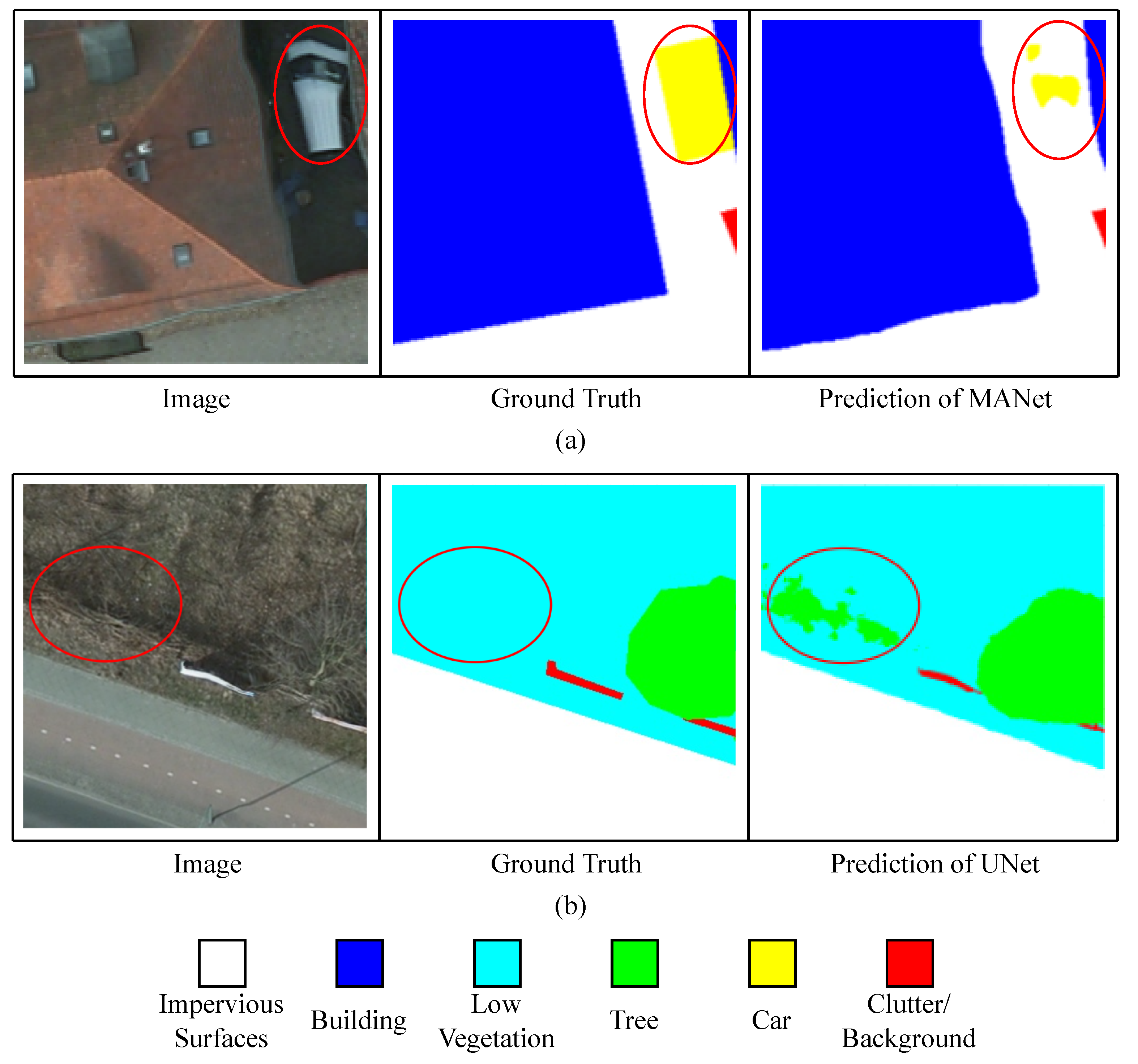
Our GMAUResNeXt reduces the problem of false segmentation and miss-segmentation in high-resolution remote sensing images by exploring interdependencies of the context and fully utilizing the multi-scale features.

The remainder of this paper is organized as follows. In Section 2, we review some related works. In Section 3, we elaborately illustrate the proposed methods. Section 4 introduces the datasets and metrics used in the experiments and comprehensively analyzes the experimental results. In Section 5, we conclude this paper and discuss the future research directions.

2. Related Work

In this section, we briefly review the approaches of semantic segmentation that are related to our work and analyze their limitations. Specifically, we first review the overall architecture used in the semantic segmentation and then discuss the attention mechanism.

2.1. Neural Network for Semantic Segmentation

There are two major architectures designed for semantic segmentation of remote sensing images: FCN-based architectures and encoder–decoder architectures. Both have brought tremendous progress in semantic segmentation. The main difference between them is that encoder–decoder architectures contain an extra symmetric expanding path that enables precise localization using the context captured by the contracting path, whereas FCN-based architectures combine semantic information from deep and coarse layers and appearance information from shallow and fine layers for detailed segmentation [26].

2.1.1. FCN-Based Architectures

In recent years, numerous FCN-based models have been proposed to compensate for the shortcomings of the original network. The image segmentation models of the DeepLabv1 series [5,27,28], proposed by Chen et al., are among the most popular. In DeepLabv3 [28], Chen et al. combines atrous convolution in cascade or in parallel to capture multi-scale context and proposes ASPP to encode global context using image-level features. However, global context information is not accounted for in an efficient manner [26]. Thus, in the final version of the DeepLab series, DeepLabv3+ employs an encoder–decoder rather than FCN-based architecture.

2.1.2. Encoder–Decoder-Based Architectures

In the encoder–decoder architecture, skip connections are employed to integrate the feature representation extracted by the encoder and decoder [12]. Most of the popular segmentation neural networks employ some sort of encoder–decoder architecture [26]. An important direction to improve the encoder–decoder structure is to refine the connection manners between the encoder and decoder [29]. Zhou et al. [6] propose UNet++, an encoder–decoder network where the encoder and decoder sub-networks are connected through a series of nested, dense skip connections. However, the skip connections are used merely at the same level of the encoder and decoder and, thus, interaction of the decoder’s upper and lower features is lacking. HRNet [30] maintains high-resolution representations through the whole process to decrease the loss of fine-grained image information. Several recent studies in semantic segmentation use HRNet as a backbone. Xu et al. [31] extends this idea to the segmentation of remote sensing images by proposing HRCNet, where global context information is obtained based on HRNet. However, the context is only extracted from the last layer of HRNet. Therefore, the multi-scale features contained in other layers of the encoder–decoder architecture are not well utilized.

2.2. Attention Mechanism

The attention mechanism is inspired by the complex cognitive function of humans that tends to let humans focus on the distinctive parts when processing a great deal of information. It has recently been widely used in deep learning. There are two learnable types of attention mechanisms: gating mechanisms and focused attention [15].

2.2.1. Focused Attention

Focused attention is applied to draw global dependencies and was first introduced to deep learning by Vaswani et al. [32] in natural language processing. Subsequently, Wang et al. [18] proposed a non-local block to adjust the scaled dot-product attention [32] for computer vision for the first time. This method has since been developed in many studies. Fu et al. [17] simultaneously consider the attention of position and channel to enhance the ability to capture global dependencies. In semantic segmentation of remote sensing, Zhang et al. [33] employ the positional attention at multiple scales to strengthen the embedding of scale-related contextual information. However, it has high spatial and time complexity due to its purpose of capturing global dependencies. To decrease the complexity to some extent with minimal compromise on performance, the convolutional block attention module (CBAM) [34], stand-alone self-attention [35], and stand-alone axial-attention [36] were proposed. Nevertheless, it is still unreasonable to use them in each layer due to their high cost, especially when dealing with large slices of high-resolution remote sensing images.

2.2.2. Gating Mechanisms

Gating mechanisms allow multiplicative interaction between a given feature vector and a gate scalar with values between 0 and 1 [23]. They are commonly used in recurrent neural networks such as GRU [37] and LSTM [38]. They have a much lower spatial and time complexity than focused attention, making the attention mechanism applied in each layer of the encoder–decoder structure feasible. Miech et al. [23] propose context gate to learn to downweight visual activations in a particular position for video classification. Oktay et al. [24] extend this idea to semantic segmentation to suppress irrelevant regions in an input feature representation while highlighting salient features useful for a specific task. However, this attention gate was used only in the same level of the encoder and decoder part, thus resulting in the global context contained in the lower layer being insufficiently used.

To fully utilize the multi-scale features and the global context generated by each lower layer of the decoder, we propose GAG based on attention gate [24] and employ GAG to connect each lower layer with the uppermost layer.

3. Methods

In this paper, we propose a global attention gate (GAG) module to capture the global context and its interdependencies implicitly contained in each layer. Based on GAG and non-local blocks, a novel neural network named global multi-attention UResNext (GMAUResNeXt) is proposed. In this section, we introduce a new semantic segmentation scheme for remote sensing images. It is found to be good at tackling context information and multi-scale features and generating attention from a global perspective, thus improving the performance of semantic segmentation architecture.

3.1. Global Multi-Attention UResNeXt

Based on GAG and non-local blocks, we design a novel network, namely the global multi-attention UResNeXt, as shown in Figure 2. We propose two versions of GMAUResNeXt: GMAUResNeXt_v1 and GMAUResNeXt_v2. As shown in Figure 3, “v1” and “v2” denote the version of GAG used in GMAUResNeXt. The difference between “v1” and “v2” is demonstrated in Section 3.2. Both GMAUResNeXt_v1 and GMAUResNeXt_v2 utilize multi-scale features by letting the lower layer of the decoder part interact with the class-score feature map of the uppermost layer and utilize the context information by using GAG in each layer from a global perspective.

To become comprehensively familiar with our model, we briefly introduce our GMAUResNeXt shown in Figure 2. We show the pipeline of semantic segmentation when inputting an image patch of shape $640\times 640\times 3$. We choose ResNeXt-101 [25] as the backbone to extract features from different scales, as it has more powerful capabilities than ResNet-101 [39]. ResNeXt-101 is constructed by repeatedly stacking bottleneck residual blocks (bottleneck shown in Figure 2). The bottleneck residual block utilizes the technique of split–convert–merge to increase accuracy when maintaining the computational complexity and size of the model. Each bottleneck residual layer extracts features from a different scale. The feature map is downsampled by using stride-2 convolutions in the 3 × 3 layer of the first block in each stage. In order to obtain global long-range dependencies with minimal computational and memory overhead, we only use non-local modules in the last layer of the backbone. After this, a global adaptive pooling layer (GAP layer) nonlinearly transforms the output from the non-local block to a global context feature vector. The low-level feature map is upsampled by the upsample layer and then concatenated with the high-level feature map extracted by each bottleneck residual layer of the ResNeXt-101. To reduce the time and spatial complexity of the model to some extent, we employ depthwise separable convolution [40] instead of vanilla convolution in the above process and upsample layers. Through the attention fusion module, we effectively utilize four attention gates generated by the GAG of each layer. We use a learnable weighted summation as the fusion method, i.e., assign a weighting coefficient to the global attention gate of each layer. It is formulated as:

$${\mathrm{a}}_{final}=\sum _{i=1}^4{\alpha }_i{a}_i,$$

(1)

where ${\mathrm{a}}_{final}$ is the final attention gate generated by the attention fusion module, ${\alpha }_i$ is the learnable coefficient, and $a_i$ is the global attention gate of each layer. Because the final attention gate considers the features of all levels of the network at the same time, it provides the attention from a global perspective. Then, we let the final attention gate provide attention to the semantic segmentation map of the last layer via the Hadamard product. The multi-scale features from each layer interact with each point of the uppermost layer of the decoder part and provide contextual information through this gating mechanism, suppressing irrelevant parts of the feature representation while enhancing salient parts. Finally, the semantic segmentation map with better performance is obtained after the Hadamard product of the final attention gate and the semantic segmentation map generated by the encoder–decoder network.

3.2. Global Attention Gate

There are interdependencies contained in the multi-scale features extracted by the neural network, and the features of the lower layer of the decoder can provide context information for the upper layer. Making full use of these characteristics will enhance the feature representation by suppressing noise introduced from regions that are irrelevant for a given class [19,20,21].

The gating mechanism was used to explore the interdependencies between feature representation to suppress useless information and enhance meaningful information, thereby improving the performance of the network. The general gating mechanism is formulated as follows:

$$Z=\sigma \left(\phi \right(X,Y\left)\right)\circ \psi \left(X\right),$$

(2)

where Z is the new feature representation, X is the input feature vector, Y is the supplementary feature vector, $\sigma$ is the element-wise sigmoid activation, and ∘ is the element-wise multiplication. $\phi (·)$ and $\psi (·)$ stand for the nonlinear transformation. $\sigma \left(\phi \right(X,Y\left)\right)$ serves as the attention gate for $\psi \left(X\right)$, thus exploring the interdependencies of X and Y.

The overall feature map of different scales, i.e., feature map from different layers, can provide attention in various global perspectives. Based on this idea, we propose GAG aiming at exploring the global context from various global perspectives. Therefore, our general gating mechanism is formulated as follows:

$$Z=\sigma \left(\phi \right(Y\left)\right)\circ \psi \left(X\right),$$

(3)

where $\phi \left(Y\right)$ stands for global context provided by each layer of the decoder part, and $\sigma \left(\phi \right(Y\left)\right)$ represents the global attention gate generated by each layer. As shown in Figure 3a, our proposed GAG is designed based on the attention gate proposed in the attention U-Net [24].

However, unlike the attention gate, we do not utilize the input feature vector in $\phi (·)$. Because $\left(\phi \right(Y)$ serves as the global context in our model, there is no need for feature fusion with X. Moreover, to utilize the context information around each pixel, we employ $3\times 3$ convolution instead of $1\times 1$ convolution in the attention gate.

To extract the global context contained in each layer and use it to generate the global attention gate, we propose two versions of GAG in this paper, as shown in Figure 3. We designed these two versions to explore whether the global context can contribute to GAG. GAG_v1 can be regarded as a simplified version of GAG_v2. GAG_v2, shown in Figure 3a, utilizes the global context generated from the GAP block, while GAG_v1, shown in Figure 3b, solely utilizes the context of each layer to generate its corresponding global attention gate. In GAG_v2, we use concatenated fusion for the feature fusion block to fuse the global context and feature map of each layer. After the concatenated features are nonlinearly transformed to global attention and upsampled, the sigmoid function is applied to generate the global attention gate. This global attention gate, which contains the context information, then provides the attention from the multiple lower layers to the uppermost layer, thus enhancing the specific salient class.

3.3. Non-Local Block

The non-local block [18] serves as a building block for capturing long-range dependencies. As shown in Figure 4, every feature vector in the feature map considers all the feature vectors in other positions.

To capture long-range dependencies and achieve the global receptive field with minimal overhead, we solely utilize the non-local block at the last layer of the encoder part of GMAUResNeXt, as shown in Figure 2.

4. Experiment

In this paper, we comprehensively evaluated our proposed method using the Potsdam dataset and GID (Gaofen image dataset). In this section, we describe the datasets, evaluation metrics, and implementation details of the experiments. We analyze the results of the performance on the Potsdam dataset and GID to demonstrate the superiority of our model.

4.1. Datasets

4.1.1. ISPRS Potsdam Dataset

The ISPRS Potsdam dataset is composed of 38 fine-resolution tiles of size $6000\times 6000$ pixels whose ground sampling distance is 5 cm. It consists of a true orthophoto (TOP) with corresponding digital surface models (DSMs). TOP has four bands, which are near-infrared (NIR), red (R), green (G), and blue (B). Six categories have been defined in the Potsdam dataset: impervious surface, building, low vegetation, tree, car, and clutter/background.

Following the settings of most research [11,22,41,42], we use 17 tiles for training, 7 tiles for validating, and the remaining 14 tiles for testing. Specifically, all 38 tiles are divided into training set (17 images, IDs: 2_10, 3_10, 3_11, 3_12, 4_11, 4_12, 5_10, 5_12, 6_8, 6_9, 6_10, 6_11, 6_12, 7_7, 7_9, 7_11, 7_12); validation set (7 images, IDs: 2_11, 2_12, 4_10, 5_11, 6_7, 7_8, 7_10); and test set (the remaining images). In addition, we use the full reference set, in which the boundary information is considered. To make full use of the training data using the strategy of multi-scale training, we set the slice size to $400\times 400$, $800\times 800$, and $1200\times 1200$ with an overlap of $50\%$ as a data augmentation strategy. During the training process, we sliced these images to $320\times 320$, $640\times 640$ and $960\times 960$. Following Yang et al. [10], we set the slice size to $960\times 960$ with an overlap of $50\%$ for the validation set and $1600\times 1600$ with no overlap for the test set.

We only utilize the RGB bands of TOP mentioned above without ground reference data lacking eroded boundaries, and the evaluation results are therefore not as high as reported in some examples in the literature.

4.1.2. Gaofen Image Dataset

The GID is collected by the Gaofen-2 Satellite in China, which has image tiles of size $7200\times 6800$ covering a geographic area of 506 km ${}^2$ [43]. It is composed of three optical bands: red (R), green (G), and blue (B). There are 15 land use categories contained in this dataset: paddy field, irrigated land, dry cropland, garden land, arbor forest, shrubland, natural meadow, artificial meadow, industrial land, urban residential, rural residential, traffic land, river, lake, and pond.

It has lower resolution and is more challenging than the Potsdam dataset. We utilize this dataset to further evaluate our proposed method. We only use one scale of data owing to its lower resolution and for evaluating the performance of our model when using the smaller image to train our model. Specifically, we split these images to the shape of $320\times 320$ with no overlap and cropped it to $256\times 256$ during the training process. We randomly selected 60% of the slice for training, 20% for validation, and the remaining 20% for testing.

4.2. Evaluation Metrics

The experiments were evaluated based on three frequently used metrics: overall accuracy (OA), mean intersection over union (mIoU), and F1 score. They are calculated as:

$$OA=\frac{{\sum }_{i=0}^k{p}_{ii}}{{\sum }_{i=0}^k{\sum }_{j=0}^k{p}_{ij}},$$

(4)

$$mIoU=\frac{1}{k+1}\sum _{i=0}^k\frac{p_{ii}}{{\sum }_{j=0}^k{p}_{ij}+{\sum }_{j=0}^k{p}_{ji}-p_{ii}},$$

(5)

$$F_1=\frac{1}{k+1}{\sum }_{i=0}^k\frac{p_{ii}}{p_{ii}+\frac{1}{2}{\sum }_{j=0}^k(p_{ij}+p_{ji})},$$

(6)

in which $p_{ii}$ represents the number of pixels of class i that are correctly classified; $p_{ij}$, which represents the number of false negatives and is the number of pixels of class i that are wrongly classified as class j; $p_{ji}$, which represents the number of false positives and is the number of pixels of class j that are wrongly classified as class i; and k is the number of categories.

4.3. Implementation Details

All of our experiments were conducted based on Pytorch using one server with one NVIDIA GeForce RTX 3090 unit of memory 24 GB. According to the same settings, our methods are compared with UNet, UResNeXt, DeepLabv3+, PSPNet, AttUNet, and FastFCN. Meanwhile, other popular methods in semantic segmentation of high-resolution remote sensing images, i.e., MANet, MDCNN, and HRCNet are also compared with GMAUResNeXt. For the Potsdam dataset, we employed multi-scale training in the training process. Specifically, we used slices of the remote sensing image of size $400\times 400$, $800\times 800$, and $1200\times 1200$. Then, we randomly cropped it to the input shape of $320\times 320$, $640\times 640$, and $960\times 960$, respectively. For the GID, we used only one scale, $256\times 256$, owing to its lower resolution and for evaluating the performance of our model when using the smaller image to train our model. As in some previous studies, we omitted the class, which is of relatively small proportion in the total number of pixels [44,45]. To avoid overfitting problems and enhance the generalization ability of our model, we utilized data augmentation, i.e., horizontal flip, vertical flip, and random crop. In the test stage, we utilized the TTA strategy [10] and sliced the large tile to $1920\times 1920$ with no overlap and fed the slices to our model. Then, we stitched the segmentation maps for the final prediction.

We trained these models without bells and whistles. Specifically, we adopted Adam as the optimizer of the learning rate $1\times {10}^{-4}$ and the batch size of $(8,4,1)$ for each scale in the Potsdam dataset. We set the batch size to 8 for the GID. For stable training, we used reduce-on-plateau as the lr-scheduler. Given the fact that pre-trained CNN weights have been found to be effective for a variety of visual tasks [46], we used the weights of ResNeXt [25] and set its learning rate as $10\%$ of the other parts of the model. We selected cross-entropy loss as the loss function and trained each model for 90 epochs.

4.4. Results on the Potsdam Dataset

We conducted numerous experiments on the Potsdam dataset to evaluate the two versions of GMAUResNeXt mentioned in Section 3.1. We compared our models with most of the classic models in the area of segmentation. Specifically, we compared our method with some classic models, i.e., UNet [12], PSPNet [47] and DeepLabv3+ [9]. Moreover, we compared our methods with three recently proposed methods in the area of semantic segmentation of remote sensing, i.e., MANet [11], MDCNN [22], and HRCNet [31]. As a result of the comprehensive comparison, the effectiveness of our proposed method was verified.

The overall experimental results on the Potsdam dataset are shown in

Table 1. The experimental results on the ISPRS Potsdam dataset. (Imp.Surf.: impervious surface; Low Veg.: low vegetation).

Method	Per-Class F1 Score					avg.F1	OA
	Imp. Surf.	Building	Low Veg.	Tree	Car
Unet [12]	88	93.52	77.76	73.43	78.18	82.18	82.81
DeepLabv3+ [9]	70.36	94.85	89.08	87.84	96.62	87.75	86.87
PSPNet [47]	70.04	95.02	88.62	87.91	96.46	87.61	87.57
UResNeXt	93.07	96.96	86.81	86.38	92.03	91.05	90.75
MANet [11]	-	-	-	-	-	89.07	88.76
MDCNN [22]	92.91	97.13	87.03	87.26	95.16	91.9	90.64
HRCNet [31]	-	-	-	-	-	90.20	89.50
GMAUResNeXt_v1	93.48	96.85	87.39	87.13	92.47	91.46	91.05
GMAUResNeXt_v2	93.71	97.26	87.82	86.78	92.88	91.69	91.32

. When considering the global context, GMAUResNeXt_v2 achieves better performance than GMAUResNeXt_v1. For per-class F1 score, our performance for all of the classes except for the “car” surpasses all other models. For the F1 score and OA, our model is slightly inferior to MDCNN in avg. F1-score but superior to MDCNN in OA by a large margin of $0.68\%$.

Compared with the UNet, a vanilla encoder–decoder structure, all the other models obtain better performance when the architecture becomes more complicated. DeepLabv3+, which uses atrous spatial pyramid pooling to aggregate the multi-scale contextual information, has the best performance among the classic models. MDCNN obtains better performance compared with the classic models by utilizing a two-stage multi-scale training architecture tailored for remote sensing images to better utilize the context information. However, these models solely fuse the feature map of the encoder and decoder at the same level. Our GMAUResNeXt captures the interdependencies of the context contained in each layer and makes full use of the information based on the multi-attention architecture.

The segmentation maps generated by these methods are illustrated in Figure 5. As circled in red, after considering the context and semantic information in each layer, GMAUResNeXt_v2 provides a more precise segmentation map than the other methods, solving the problems of false segmentation and miss-segmentation.

Although the overall performance of GMAUResNeXt is superior to that of other models, the F1 score for “car” is vastly inferior to that of MDCNN. This may be caused by data imbalance. We visualized the confusion matrix, as shown in Figure 6. In the confusion matrix, we found that the number of pixels of “car” of the test set is at a scale of $1\times {10}^6$, whereas all the other classes except for the “background/clutter” are at a scale of $1\times {10}^7$.

4.5. Results on the GID Dataset

To further evaluate our proposed method, we chose GID, which is more challenging than the Potsdam dataset. It has 15 classes of land use classes of lower resolution than the Potsdam dataset. To fairly compare GMAUResNeXt with the other models, we adopt the same experimental settings given by Li et al. [11] without using the TTA strategy. We compared our mehod with some classic models, i.e., UNet [12], AttUNet [24], FastFCN [48], PSPNet [47], and DeepLabv3+ [9].

The quantative results are shown in shown in

Table 2. The experimental results on the GID dataset.

Method	OA	mIoU	F1
UNet [12]	86.29	78.88	87.56
AttUNet [24]	85.47	78.19	87.17
UResNeXt	87.88	79.68	88.22
DeepLabv3+ [9]	85.00	74.88	84.69
FastFCN [48]	81.23	72.15	82.58
PSPNet [47]	82.79	74.61	84.57
MANet [11]	86.51	78.33	87.14
GMAUResNeXt_v2	89.70	83.22	90.51

. As we can see, GMAUResNeXt_v2 surpasses all the classic architectures and exceeds MANet [11] by a large margin, with a 3.19% improvement in OA, 4.89% improvement in mIoU, and 3.19% improvement in F1. The visualization results, which demonstrate the superiority of our method, are shown in Figure 7.

4.6. Comparison of Complexity

We further analyze the number of trainable parameters and computational complexity and training time (including training and validating) of GMAUResNeXt_v2 with other models on the Potsdam and GID datasets. The results are shown in

Table 3. The comparison of trainable parameters, computational complexity, and training time (hours) on the Potsdam dataset. ‘M’ represents million, ‘GFLOPs’ represents giga floating-point operations. GFLOPs(size) means the shape of the input is 3 × size × size when counting the GFLOPs.

Method	Params (M)	GFLOPs (320)	GFLOPs (640)	GFLOPs (960)	Training Time
UNet [12]	31.03	75.52	302.07	679.66	13.98
DeepLabv3+ [9]	59.47	37.57	150.27	338.1	11.04
PSPNet [47]	65.71	89.29	357.18	803.59	14.18
UResNeXt	93.78	42.34	169.35	381.02	11.00
MANet [11]	93.65	39.37	157.48	354.33	-
MDCNN [22]	-	-	-	-	-
HRCNet [31]	59.8	-	-	-	-
GMAUResNeXt_v1	108.00	44.93	179.96	405.82	11.71
GMAUResNeXt_v2	110.06	45.95	184.04	415.02	13.46

and

Table 4. The comparison of trainable parameters, computational complexity, and training time (hours) on the GID dataset. ‘M’ represents million, ‘GFLOPs’ represents giga floating-point operations. The shape of the input is 3 × 256 × 256.

Method	Params (M)	GFLOPs	Training Time
UNet [12]	31.03	48.33	2.07
AttUNet [24]	34.88	66.74	1.65
UResNeXt	93.78	27.10	2.03
DeepLabv3+ [9]	59.47	24.07	2.12
FastFCN [9]	104.30	70.59	1.92
PSPNet [47]	65.71	89.29	2.10
MANet [11]	93.65	25.73	-
GMAUResNeXt	110.06	29.40	2.18

. Some metrics of some models are not taken into account, since the source codes of MANet, MDCNN, and HRCNet are not publicly available.

The number of trainable parameters and computational complexity of GMAUResNeXt_v2 is reasonable when considering the much better performance on Potsdam and GID. Specifically, compared with the baseline UResNeXt on GID, GMAUResNeXt has a 3.58% improvement in mIoU with only an overhead of 16.28 M parameters and 2.3 GFLOPs. The computational complexity of GMAUResNeXt_v2 is considerably smaller than of FastFCN, PSPNet, AttUNet, and UNet and comparable to other classic models. Moreover, it is not costly to train GMAUResNeXt both on Potsdam and GID, taking only 2.18 and 13.46 h, respectively, for training GMAUResNeXt_v2 for 90 epochs on GID and Potsdam with one NVIDIA GeForce RTX 3090 unit with 24 GB of memory.

5. Discussion

To further explore the effectiveness of our proposed methods, we conducted an extensive ablation study and visualize the GAG output. The results of the ablation study and GAG visualization demonstrate its effectiveness.

5.1. Ablation Study of GAG

To quantitatively validate our proposed GAG and study the effects of GAG applied on each layer, we conducted an extensive ablation study. Specifically, we chose four versions of GMAUResNeXt_v2 and a plain UResNeXt for this experiment, as shown in

Table 5. The ablation study of the GAG on the ISPRS Potsdam dataset.

Method	Per-Class F1 Score					avg.F1	OA
	Imp. Surf.	Building	Low Veg.	Tree	Car
UResNeXt	93.07	96.96	86.81	86.38	92.03	91.05	90.75
GMAUResNeXt_1	93.35	97.18	87.47	86.83	92.04	91.37	90.71
GMAUResNeXt_2	93.73	97.26	87.67	86.91	92.73	91.66	91.23
GMAUResNeXt_3	93.81	97.13	87.49	86.95	93.16	91.71	91.44
GMAUResNeXt_v2	93.71	97.26	87.82	86.78	92.88	91.69	91.32

. The number in the suffix shown in the table denotes the number of GAG blocks to be removed from the bottom of the architecture. For example, GMAUResNeXt_2 means removing the last two GAG blocks from the bottom of the architecture.

The experimental results of the ablation study are shown in Table 5. To our surprise, only using the uppermost GAG block of the GMAUResNeXt_v2 obtains the best result, which is $0.66\%$ higher than the baseline UResNeXt in avg. F1 and has a $0.69\%$ improvement in OA. Removing the first GAG block from the bottom of the architecture brings about a $0.3\%$ decrease in avg. F1 and $0.6\%$ in OA. However, when gradually removing the other GAG blocks, the performance improves, and the best result is obtained when solely using the uppermost GAG block, which has a performance similar to the complete GMAUResNeXt_v2.

However, the four GAG blocks in the GMAUResNeXt_v2 do learn different attention patterns, as demonstrated in Section 5.2. We considered that the reason for these experimental results is that the aggregating method of fusing all the attention generated by each block is simple and not effective. Moreover, the nonlinear transformation used in the GAG may be not complicated enough to adequately transform the context contained in each layer into attention.

5.2. Visualization of GAG

We conducted a qualitative experiment to analyze the effect of GAG. We visualized the global attention gate generated by each GAG block. Specifically, we visualized the global attention gate generated by GMAUResNeXt_v2 on the Potsdam dataset.

For the Potsdam dataset, we separately visualized the global attention gate and the final attention gate of three categories generated by the GAG. Specifically, we visualized the global attention gate of two confusing classes to show the effects of the GAG. Moreover, we visualized the global attention gate of the “Car” class, which has only about one-tenth the amount of training samples of other categories in the Potsdam dataset.

As shown in Figure 8a,b, for some cases, it is hard even for experts to recognize the difference between “tree” and “low vegetation” in the Potsdam dataset. However, GAG makes plenty use of the context and the interdependencies contained in the feature map of different layers, thus making these categories more separable. As we can see, in Figure 8a,b, different GAGs provide different attention of where to focus on and where to ignore. For the global attention gate of the “tree” class, it enhances the “tree” part in the RS images and attenuates the part of the other categories such as “low vegetation”. As for the ground objects shown in Figure 8b circled in red, after the depressing effects of the GAG, it solves the problem mentioned in Figure 8b. Moreover, we found a phenomenon that at the lower part of the decoder, GAG tends to provide a rough outline of attention and it provides a finer outline of attention at the upper part of the decoder. We considered that increasing the ability of nonlinear transformation of GAG will make it generate a more accurate outline at the lower part, thus improving the performance, due to the fact that GAG at the lower part provides attention from a different global point of view. Another defect of GAG is that it cannot cope well with the problem of data imbalance. As shown in Figure 8c, it hardly learns any useful information. Therefore, it treats all categories equally so as not to cause damage to the performance.

6. Conclusions

In this paper, we propose an attention module named GAG to capture the potential interdependencies of the context contained in each layer of the encoder–decoder architecture from a global point of view. Based on GAG, we designed a novel GMAUResNeXt to utilize the interdependencies and long-range dependencies of the context contained in each layer. GMAUResNeXt utilizes multi-scale features and exploits the interdependencies and long-range dependencies of the context contained in each layer to enhance the capability of feature representation for the encoder–decoder architecture. GMAUResNeXt outperformed the classic semantic segmentation models and other popular approaches used in high-resolution remote sensing images, outperforming MDCNN by 0.68% on the Potsdam dataset and MANet by 3.19% on GID in terms of the overall accuracy. Moreover, the visualization results demonstrate the effectiveness of GAG. Although the effectiveness and superiority of the performance of our proposed methods were demonstrated through numerous experiments, some limitations still exist. One of the limitations of our proposed methods is that it will still take a large amount of memory when the slice of the high-resolution remote sensing image increases. The other is that GMAUResNeXt cannot deal well with the data imbalance. In future, we will consider how to decrease memory usage while maintaining the capability of GAG, and how to solve the problem of data imbalance should be explored.

References

1. Yuan, X.; Sarma, V. Automatic Urban Water-Body Detection and Segmentation From Sparse ALSM Data via Spatially Constrained Model-Driven Clustering. IEEE Geosci. Remote Sens. Lett. 2011, 8, 73–77. [Google Scholar] [CrossRef]
2. Zhang, J.; Feng, L.; Yao, F. Improved maize cultivated area estimation over a large scale combining MODIS–EVI time series data and crop phenological information. ISPRS J. Photogramm. Remote Sens. 2014, 94, 102–113. [Google Scholar] [CrossRef]
3. Yang, S.; Chen, Q.; Yuan, X.; Liu, X. Adaptive Coherency Matrix Estimation for Polarimetric SAR Imagery Based on Local Heterogeneity Coefficients. IEEE Trans. Geosci. Remote Sens. 2016, 54, 6732–6745. [Google Scholar] [CrossRef]
4. Krizhevsky, A.; Sutskever, I.; Hinton, G.E. ImageNet Classification with Deep Convolutional Neural Networks. In Proceedings of the Advances in Neural Information Processing Systems, Lake Tahoe, NV, USA, 3–6 December 2012; Pereira, F., Burges, C., Bottou, L., Weinberger, K., Eds.; Curran Associates, Inc.: New York, NY, USA, 2012; Volume 25. [Google Scholar]
5. Chen, L.C.; Papandreou, G.; Kokkinos, I.; Murphy, K.; Yuille, A.L. DeepLab: Semantic Image Segmentation with Deep Convolutional Nets, Atrous Convolution, and Fully Connected CRFs. IEEE Trans. Pattern Anal. Mach. Intell. 2018, 40, 834–848. [Google Scholar] [CrossRef] [Green Version]
6. Zhou, Z.; Rahman Siddiquee, M.M.; Tajbakhsh, N.; Liang, J. UNet++: A Nested U-Net Architecture for Medical Image Segmentation. In Proceedings of the Deep Learning in Medical Image Analysis and Multimodal Learning for Clinical Decision Support, Granada, Spain, 20 September 2018; Springer International Publishing: Cham, Switzerland, 2018; pp. 3–11. [Google Scholar]
7. Guo, Y.; Liu, Y.; Georgiou, T.; Lew, M.S. A review of semantic segmentation using deep neural networks. Int. J. Multimed. Inf. Retr. 2018, 7, 87–93. [Google Scholar] [CrossRef] [Green Version]
8. Asgari Taghanaki, S.; Abhishek, K.; Cohen, J.P.; Cohen-Adad, J.; Hamarneh, G. Deep semantic segmentation of natural and medical images: A review. Artif. Intell. Rev. 2021, 54, 137–178. [Google Scholar] [CrossRef]
9. Chen, L.C.; Zhu, Y.; Papandreou, G.; Schroff, F.; Adam, H. Encoder-Decoder with Atrous Separable Convolution for Semantic Image Segmentation. In Proceedings of the European Conference on Computer Vision (ECCV), Munich, Germany, 8–14 September 2018; pp. 801–818. [Google Scholar]
10. Yang, X.; Li, S.; Chen, Z.; Chanussot, J.; Jia, X.; Zhang, B.; Li, B.; Chen, P. An attention-fused network for semantic segmentation of very-high-resolution remote sensing imagery. ISPRS J. Photogramm. Remote Sens. 2021, 177, 238–262. [Google Scholar] [CrossRef]
11. Li, R.; Zheng, S.; Zhang, C.; Duan, C.; Su, J.; Wang, L.; Atkinson, P.M. Multiattention Network for Semantic Segmentation of Fine-Resolution Remote Sensing Images. IEEE Trans. Geosci. Remote Sens. 2022, 60, 1–13. [Google Scholar] [CrossRef]
12. Ronneberger, O.; Fischer, P.; Brox, T. U-Net: Convolutional Networks for Biomedical Image Segmentation. In Proceedings of the Medical Image Computing and Computer-Assisted Intervention—MICCAI 2015, Munich, Germany, 5–9 October 2015; Springer International Publishing: Berlin/Heidelberg, Germany, 2015; pp. 234–241. [Google Scholar]
13. Yu, W.; Yang, K.; Yao, H.; Sun, X.; Xu, P. Exploiting the complementary strengths of multi-layer CNN features for image retrieval. Neurocomputing 2017, 237, 235–241. [Google Scholar] [CrossRef]
14. Corbetta, M.; Shulman, G.L. Control of goal-directed and stimulus-driven attention in the brain. Nat. Rev. Neurosci. 2002, 3, 201–215. [Google Scholar] [CrossRef]
15. Niu, Z.; Zhong, G.; Yu, H. A review on the attention mechanism of deep learning. Neurocomputing 2021, 452, 48–62. [Google Scholar] [CrossRef]
16. Cho, K.; Merrienboer, B.V.; Gulcehre, C.; Bougares, F.; Schwenk, H.; Bengio, Y. Learning Phrase Representations using RNN Encoder-Decoder for Statistical Machine Translation. In Proceedings of the EMNLP, Doha, Qatar, 25–29 October 2014. [Google Scholar]
17. Fu, J.; Liu, J.; Tian, H.; Li, Y.; Bao, Y.; Fang, Z.; Lu, H. Dual Attention Network for Scene Segmentation. In Proceedings of the IEEE/CVF Conference on Computer Vision and Pattern Recognition (CVPR), Long Beach, CA, USA, 15–20 June 2019. [Google Scholar]
18. Wang, X.; Girshick, R.; Gupta, A.; He, K. Non-Local Neural Networks. In Proceedings of the IEEE Conference on Computer Vision and Pattern Recognition (CVPR), Salt Lake City, UT, USA, 18–23 June 2018. [Google Scholar]
19. Yang, Z.; He, X.; Gao, J.; Deng, L.; Smola, A. Stacked Attention Networks for Image Question Answering. In Proceedings of the IEEE Conference on Computer Vision and Pattern Recognition (CVPR), Las Vegas, NV, USA, 27–30 June 2016. [Google Scholar]
20. Yu, Y.; Ji, Z.; Fu, Y.; Guo, J.; Pang, Y.; Zhang, Z.M. Stacked Semantics-Guided Attention Model for Fine-Grained Zero-Shot Learning. In Proceedings of the Advances in Neural Information Processing Systems, Montréal, QC, Canada, 3–8 December 2018; Curran Associates, Inc.: New York, NY, USA, 2018; Volume 31. [Google Scholar]
21. Sinha, A.; Dolz, J. Multi-Scale Self-Guided Attention for Medical Image Segmentation. IEEE J. Biomed. Health Inform. 2021, 25, 121–130. [Google Scholar] [CrossRef] [PubMed] [Green Version]
22. Ding, L.; Zhang, J.; Bruzzone, L. Semantic Segmentation of Large-Size VHR Remote Sensing Images Using a Two-Stage Multiscale Training Architecture. IEEE Trans. Geosci. Remote Sens. 2020, 58, 5367–5376. [Google Scholar] [CrossRef]
23. Miech, A.; Laptev, I.; Sivic, J. Learnable pooling with context gating for video classification. arXiv 2017, arXiv:1706.06905. [Google Scholar]
24. Oktay, O.; Schlemper, J.; Folgoc, L.L.; Lee, M.; Heinrich, M.; Misawa, K.; Mori, K.; McDonagh, S.; Hammerla, N.Y.; Kainz, B.; et al. Attention u-net: Learning where to look for the pancreas. arXiv 2018, arXiv:1804.03999. [Google Scholar]
25. Xie, S.; Girshick, R.; Dollar, P.; Tu, Z.; He, K. Aggregated Residual Transformations for Deep Neural Networks. In Proceedings of the IEEE Conference on Computer Vision and Pattern Recognition (CVPR), Honolulu, HI, USA, 21–26 July 2017. [Google Scholar]
26. Minaee, S.; Boykov, Y.; Porikli, F.; Plaza, A.; Kehtarnavaz, N.; Terzopoulos, D. Image Segmentation Using Deep Learning: A Survey. IEEE Trans. Pattern Anal. Mach. Intell. 2022, 44, 3523–3542. [Google Scholar] [CrossRef]
27. Chen, L.C.; Papandreou, G.; Kokkinos, I.; Murphy, K.; Yuille, A.L. Semantic image segmentation with deep convolutional nets and fully connected crfs. arXiv 2014, arXiv:1412.7062. [Google Scholar]
28. Chen, L.C.; Papandreou, G.; Schroff, F.; Adam, H. Rethinking atrous convolution for semantic image segmentation. arXiv 2017, arXiv:1706.05587. [Google Scholar]
29. Diakogiannis, F.I.; Waldner, F.; Caccetta, P.; Wu, C. ResUNet-a: A deep learning framework for semantic segmentation of remotely sensed data. ISPRS J. Photogramm. Remote Sens. 2020, 162, 94–114. [Google Scholar] [CrossRef] [Green Version]
30. Sun, K.; Xiao, B.; Liu, D.; Wang, J. Deep High-Resolution Representation Learning for Human Pose Estimation. In Proceedings of the IEEE/CVF Conference on Computer Vision and Pattern Recognition (CVPR), Long Beach, CA, USA, 15–20 June 2019. [Google Scholar]
31. Xu, Z.; Zhang, W.; Zhang, T.; Li, J. HRCNet: High-Resolution Context Extraction Network for Semantic Segmentation of Remote Sensing Images. Remote Sens. 2021, 13, 71. [Google Scholar] [CrossRef]
32. Vaswani, A.; Shazeer, N.; Parmar, N.; Uszkoreit, J.; Jones, L.; Gomez, A.N.; Kaiser, L.u.; Polosukhin, I. Attention is All you Need. In Proceedings of the Advances in Neural Information Processing Systems, Long Beach, CA, USA, 4–9 December 2017; Curran Associates, Inc.: New York, NY, USA, 2017; Volume 30. [Google Scholar]
33. Zhang, J.; Lin, S.; Ding, L.; Bruzzone, L. Multi-Scale Context Aggregation for Semantic Segmentation of Remote Sensing Images. Remote Sens. 2020, 12, 701. [Google Scholar] [CrossRef] [Green Version]
34. Woo, S.; Park, J.; Lee, J.Y.; Kweon, I.S. CBAM: Convolutional Block Attention Module. In Proceedings of the European Conference on Computer Vision (ECCV), Munich, Germany, 8–14 September 2018. [Google Scholar]
35. Ramachandran, P.; Parmar, N.; Vaswani, A.; Bello, I.; Levskaya, A.; Shlens, J. Stand-Alone Self-Attention in Vision Models. In Proceedings of the Advances in Neural Information Processing Systems, Vancouver, BC, Canada, 8–14 December 2019; Curran Associates, Inc.: New York, NY, USA, 2019; Volume 32. [Google Scholar]
36. Wang, H.; Zhu, Y.; Green, B.; Adam, H.; Yuille, A.; Chen, L.C. Axial-DeepLab: Stand-Alone Axial-Attention for Panoptic Segmentation. In Proceedings of the Computer Vision—ECCV 2020, Glasgow, UK, 23–28 August 2020; Springer International Publishing: Cham, Switzerland, 2020; pp. 108–126. [Google Scholar]
37. Cho, K.; Van Merriënboer, B.; Bahdanau, D.; Bengio, Y. On the properties of neural machine translation: Encoder-decoder approaches. arXiv 2014, arXiv:1409.1259. [Google Scholar]
38. Hochreiter, S.; Schmidhuber, J. Long Short-Term Memory. Neural Comput. 1997, 9, 1735–1780. [Google Scholar] [CrossRef]
39. He, K.; Zhang, X.; Ren, S.; Sun, J. Deep Residual Learning for Image Recognition. In Proceedings of the IEEE Conference on Computer Vision and Pattern Recognition (CVPR), Las Vegas, NV, USA, 27–30 June 2016. [Google Scholar]
40. Chollet, F. Xception: Deep Learning With Depthwise Separable Convolutions. In Proceedings of the IEEE Conference on Computer Vision and Pattern Recognition (CVPR), Honolulu, HI, USA, 21–26 July 2017. [Google Scholar]
41. Wang, Y.; Liang, B.; Ding, M.; Li, J. Dense Semantic Labeling with Atrous Spatial Pyramid Pooling and Decoder for High-Resolution Remote Sensing Imagery. Remote Sens. 2019, 11, 20. [Google Scholar] [CrossRef] [Green Version]
42. Land cover mapping at very high resolution with rotation equivariant CNNs: Towards small yet accurate models. ISPRS J. Photogramm. Remote Sens. 2018, 145, 96–107. [CrossRef] [Green Version]
43. Tong, X.Y.; Xia, G.S.; Lu, Q.; Shen, H.; Li, S.; You, S.; Zhang, L. Land-cover classification with high-resolution remote sensing images using transferable deep models. Remote Sens. Environ. 2020, 237, 111322. [Google Scholar] [CrossRef] [Green Version]
44. Marmanis, D.; Schindler, K.; Wegner, J.; Galliani, S.; Datcu, M.; Stilla, U. Classification with an edge: Improving semantic image segmentation with boundary detection. ISPRS J. Photogramm. Remote Sens. 2018, 135, 158–172. [Google Scholar] [CrossRef] [Green Version]
45. Zhang, C.; Sargent, I.; Pan, X.; Gardiner, A.; Hare, J.; Atkinson, P.M. VPRS-Based Regional Decision Fusion of CNN and MRF Classifications for Very Fine Resolution Remotely Sensed Images. IEEE Trans. Geosci. Remote Sens. 2018, 56, 4507–4521. [Google Scholar] [CrossRef] [Green Version]
46. Sherrah, J. Fully convolutional networks for dense semantic labelling of high-resolution aerial imagery. arXiv 2016, arXiv:1606.02585. [Google Scholar]
47. Zhao, H.; Shi, J.; Qi, X.; Wang, X.; Jia, J. Pyramid Scene Parsing Network. In Proceedings of the IEEE Conference on Computer Vision and Pattern Recognition (CVPR), Honolulu, HI, USA, 21–26 July 2017. [Google Scholar]
48. Wu, H.; Zhang, J.; Huang, K.; Liang, K.; Yu, Y. Fastfcn: Rethinking dilated convolution in the backbone for semantic segmentation. arXiv 2019, arXiv:1903.11816. [Google Scholar]
Figure 1. Examples of the prediction of cropped images of shape 256 × 256 from the Potsdam dataset using some popular semantic segmentation methods: (a) wrong prediction of the “car”, circled in red, using MANet; (b) wrong prediction of the “low vegetation”, circled in red, using UNet.
Remotesensing 15 01836 g001
Figure 2. Schematic of the GMAUResNeXt_v2.
Remotesensing 15 01836 g002
Figure 3. Illustration of global attention gate: (a) GAG_v1 and (b) GAG_v2.
Remotesensing 15 01836 g003
Figure 4. A space non-local block. H, W, and C stands for the height, width, and channel, respectively, of the feature map. The blue box stands for 1 × 1 convolution. “⊗” denotes matrix multiplication, and “⊕” denotes element-wise sum.
Remotesensing 15 01836 g004
Figure 5. Qualitative comparisons of the segmentation results for the Potsdam dataset generated by different semantic segmentation approaches.
Remotesensing 15 01836 g005
Figure 6. The confusion matrix for the Potsdam dataset using GMAUResNeXt_v2. The number in the confusion matrix refers to the number of pixels of ground truth predicted for a specific class. The rightmost column indicates the overall accuracy and the total number of pixels for a certain ground object.
Remotesensing 15 01836 g006
Figure 7. Qualitative comparisons of the segmentation results for the GID generated by different semantic segmentation approaches.
Remotesensing 15 01836 g007
Figure 8. Visualization of the global attention gate for the Potsdam dataset generated by GAG using GMAUResNeXt_v2. Each heatmap corresponds to a specific class. GAG_1 denotes the global attention gate is generated by the GAG_1 shown in Figure 2. GAG_final denotes the final attention gate generated by the attention fusion module combining the information of the global attention gate of four GAGs.
Remotesensing 15 01836 g008aRemotesensing 15 01836 g008b