Article

Evaluation of MODIS, Landsat 8 and Sentinel-2 Data for Accurate Crop Yield Predictions: A Case Study Using STARFM NDVI in Bavaria, Germany

by
Maninder Singh Dhillon
1,*,
Carina Kübert-Flock
2,
Thorsten Dahms
1,3,
Thomas Rummler
4,
Joel Arnault
5,
Ingolf Steffan-Dewenter
6 and
Tobias Ullmann
1
1
Department of Remote Sensing, Institute of Geography and Geology, University of Würzburg, 97074 Würzburg, Germany
2
Department of Remote Sensing, Hessian State Agency for Nature Conservation, Environment and Geology (HLNUG), 65203 Wiesbaden, Germany
3
Gauss Center for Geodesy and Geoinformation, Federal Agency for Cartography and Geodesy, 60598 Frankfurt am Main, Germany
4
Department of Applied Computer Science, Institute of Geography, University of Augsburg, 86159 Augsburg, Germany
5
Institute of Meteorology and Climate Research, Karlsruhe Institute of Technology, Campus Alpin, 82467 Garmisch-Partenkirchen, Germany
6
Department of Animal Ecology and Tropical Biology, University of Würzburg, 97074 Würzburg, Germany
*
Author to whom correspondence should be addressed.
Remote Sens. 2023, 15(7), 1830; https://doi.org/10.3390/rs15071830
Submission received: 17 February 2023 / Revised: 23 March 2023 / Accepted: 25 March 2023 / Published: 29 March 2023
(This article belongs to the Special Issue Monitoring Crops and Rangelands Using Remote Sensing)

Abstract

:
The increasing availability and variety of global satellite products and the rapid development of new algorithms has provided great potential to generate a new level of data with different spatial, temporal, and spectral resolutions. However, the ability of these synthetic spatiotemporal datasets to accurately map and monitor our planet on a field or regional scale remains underexplored. This study aimed to support future research efforts in estimating crop yields by identifying the optimal spatial (10 m, 30 m, or 250 m) and temporal (8 or 16 days) resolutions on a regional scale. The current study explored and discussed the suitability of four different synthetic (Landsat (L)-MOD13Q1 (30 m, 8 and 16 days) and Sentinel-2 (S)-MOD13Q1 (10 m, 8 and 16 days)) and two real (MOD13Q1 (250 m, 8 and 16 days)) NDVI products combined separately to two widely used crop growth models (CGMs) (World Food Studies (WOFOST), and the semi-empiric Light Use Efficiency approach (LUE)) for winter wheat (WW) and oil seed rape (OSR) yield forecasts in Bavaria (70,550 km2) for the year 2019. For WW and OSR, the synthetic products’ high spatial and temporal resolution resulted in higher yield accuracies using LUE and WOFOST. The observations of high temporal resolution (8-day) products of both S-MOD13Q1 and L-MOD13Q1 played a significant role in accurately measuring the yield of WW and OSR. For example, L- and S-MOD13Q1 resulted in an R2 = 0.82 and 0.85, RMSE = 5.46 and 5.01 dt/ha for WW, R2 = 0.89 and 0.82, and RMSE = 2.23 and 2.11 dt/ha for OSR using the LUE model, respectively. Similarly, for the 8- and 16-day products, the simple LUE model (R2 = 0.77 and relative RMSE (RRMSE) = 8.17%) required fewer input parameters to simulate crop yield and was highly accurate, reliable, and more precise than the complex WOFOST model (R2 = 0.66 and RRMSE = 11.35%) with higher input parameters. Conclusively, both S-MOD13Q1 and L-MOD13Q1, in combination with LUE, were more prominent for predicting crop yields on a regional scale than the 16-day products; however, L-MOD13Q1 was advantageous for generating and exploring the long-term yield time series due to the availability of Landsat data since 1982, with a maximum resolution of 30 m. In addition, this study recommended the further use of its findings for implementing and validating the long-term crop yield time series in different regions of the world.

1. Introduction

Crop yields play a significant role in the world’s agricultural development; however, the combined effects of climate change, increase in global population, and degradation of soil and water resources requires main methods that provide a timely and accurate assessment of crop production and contribute towards increasing the sustainability of agricultural food production [1,2,3]. Over the past few years, the growth in publicly available satellite data and the emergence of new technologies has provided the potential to generate and explore a new level of data with different spatial, temporal, and spectral resolutions [4,5,6,7,8]. However, the fundamental requirements of newly generated synthetic data, i.e., their optimal spatial or temporal resolutions in accurately predicting crop yields, still need to be explored [4,9,10].
To ensure the accurate monitoring of crop yields, many studies in the past two decades have started to examine the relationship between plants and their growing environment and proposed crop models to simulate the crop growth status [11,12,13,14,15,16,17,18]. Since then, crop models have advanced in monitoring crop growth from the qualitative to the quantitative level and have been modified from the simulation of the growth process at a plant level to the field or regional level. Over time, crop growth models (CGMs) such as World Food Studies (WOFOST), Agricultural Production Systems Simulator (APSIM), AquaCrop, Cropping Systems Simulation Model (CropSyst), and Light Use Efficiency (LUE) have been refined and updated to simulate better crop growth status and yield [5,11,15,17,18,19,20,21,22]. However, when crop yields are examined at field scales, CGMs need to account for the spatial variation by providing the spatial distribution of climate variables (temperature, precipitation, soil moisture) and biophysical parameters (leaf area index (LAI), biomass, fraction of absorbed photosynthetic active radiation (FPAR)) [23]. The unavailability of spatial information in crop modelling causes uncertainties that affect the whole model’s physiological growth simulation process and leads to more significant errors in crop yield estimation [19,24].
As an alternative, the remote sensing (RS) approach can fill the spatial gap of CGMs by providing timely, ubiquitous, and frequent observations of the land surface at a range of spatial scales [24]. However, having the marked advantages, the RS approach also has important disadvantages. Optical RS data can suffer from significant gaps in the data record due to the cloud and shadow cover that causes uncertainties in the retrieved set of parameters [4,25,26]. Moreover, RS data is limited to only retrieving a few variables of interest, limiting its potential for accurately monitoring agricultural applications [27,28,29]. On the other hand, because of the heterogeneity in agricultural landscapes (various crop and soil types), CGMs have trouble parameterising for large-scale applications. Thus, to accurately monitor crop phenology and improve crop models’ results, combining CGMs and RS data is desirable to obtain the suitability of both realms [5,30]. Many studies have successfully utilised RS-based LAI or FPAR derived from vegetation indices, e.g., the Normalised Difference Vegetation Index (NDVI), in combination with CGMs to estimate crop biomass or yield at different study regions worldwide [5,31,32,33,34,35,36,37,38,39].
For five decades, the availability of RS data has grown historically, globally, and technically in terms of different spatial, temporal, and spectral resolutions, which has created new possibilities for generating accurate datasets for agricultural monitoring [4,5,40]. However, the significant cloud- and shadow-generated gaps in freely available satellite products (such as Landsat and Sentinel-2) hinders RS applications’ accurate and timely-dense monitoring. Therefore, filling the data gaps in the RS input data is more realistic before implementing the synergistic approach (where CGMs are linked with the RS data) for crop monitoring.
To fill the observation gaps in the RS data, spatial-temporal data fusion, where a high spatial resolution product is synchronised with a coarse or low-resolution product, is considered the most effective solution recommended by many studies on detecting vegetation changes [41,42,43,44]. The Spatial and Temporal Adaptive Reflectance Fusion Model (STARFM), which blends the coarse spatial resolution of MODIS and high spatial resolution of Landsat data, was the first initiative in fusion modelling. Since then, many spatiotemporal models have been developed with a successful validation of new synthetic data [6,7,8,45,46,47,48,49]. Moreover, generating new-resolution synthetic products provides geoscience applications with multi-spatial and multi-temporal resolution data. It then outputs different spatial and temporal data of the ground objects [4,5]. However, the potential of newly generated synthetic data obtained from fusion modelling in crop yield predictions using crop modelling still needs to be explored. Inputting RS data with high spatial and temporal resolution could be further used to improve the time series simulation of crop models and increase the models’ simulation accuracy. In addition, the high spatial resolution of RS data could be used to reduce the problem of mixed pixels and then increase the accuracy of different spatial properties at the field scale [19].
In the current study, the STARFM-based synthetic NDVI time series for the application of agriculture is selected from [4,5], where the fusion of MOD13Q1 (20 m, 16 days) is individually achieved with Landsat (30 m, 16 days; L) and Sentinel-2 (10 m, 5–6 days; S). Therefore, intending to investigate the importance of synthetic and real NDVI products with a different spatial and temporal resolutions, this research paper compares other output products which calculate the crop yield of winter wheat (WW) and oil seed rape (OSR) for Bavaria in 2019. The crop yield output of six different RS products (real: MOD13Q1 (250 m, 8 and 16 days); synthetic: L-MOD13Q1 (30 m, 8 and 16 days) and S-MOD13Q1 (10 m, 8 and 16 days)) with two widely used CGMs (WOFOST and LUE), for the respective crops, is tested. Eventually, for accurate crop yield modelling of WW and OSR in 2019, this study answers three research questions:
  • What is the optimal spatial resolution (10 m, 30 m, or 250 m)?
  • What is the optimal temporal resolution (8 or 16 days)?
  • Which is the suitable CGM (LUE or WOFOST)?
Investigating RS products’ optimal spatial and temporal resolutions for accurate crop yield predictions using CGMs requires heavy preprocessing of multiple synthetic and non-synthetic remote sensing datasets. Therefore, knowing the suitable data inputs for crop modelling would save time and computation power for future crop yield prediction and precision farming studies.

2. Materials and Methods

The general workflow of this study is shown in Figure 1. The flow diagram is divided into (1) Data fusion and (2) Crop yield modelling for 2019. The first part was a testing phase that investigated the suitable synthetic NDVI products (which were L-MOD13Q1 and S-MDO13Q1) for the agricultural land cover class of Bavaria for the year 2019 (completed in the preceding work [4]). The “index-then-blend” (IB) technique is used in the previous study to first produce the NDVI from the high pair (Landsat or Sentinel-2) and low pair (MOD13Q1) images before blending them for the data fusion [50]. The IB technique combines only one band, the NDVI. Therefore, it was faster and less expensive to compute. In the second section, the selected output NDVI time series of part 1 (two real: MOD13Q1 (250 m, 8 and 16 days) and four synthetic: L-MOD13Q1 (30 m, 8 and 16 days) and S-MOD13Q1 (10 m, 8 and 16 days)) and the climate elements were used as an input to the LUE and WOFOST models estimating the crop yield of WW and OSR for 2019 in Bavaria. The satellite NDVI and the climate data were selected for the respective start and end of the season for WW and OSR for 2019. Both inputs are masked for WW and OSR using the InVeKos data (source: www.ec.europa.eu/info/index_en, accessed on 21 June 2021).
In the last steps, Bavaria’s obtained crop yield is validated using the Bayerisches Landesamt für Statistik (LfStat) data at the regional level (with a 95% confidence interval). The satellite datasets were downloaded and preprocessed in Google Earth Engine (GEE), and the fusion analysis was performed in R (version 4.0.3) using RStudio.

2.1. Study Area

The federal state of Bavaria is located between 47°N and 50.5°N and between 9°E and 14°E in the southeastern part of Germany (Figure 2). The topography mainly influences the region’s climate, with higher elevations in the south (northern edge of the Alps) and east (Bavarian Forest and Fichtel Mountains). The mean annual temperature ranges from −3.3 to 11 °C, but in most of the territory, the temperature ranges between 8 and 10 °C [4]. The mean annual precipitation sums range from approximately 500 to above 3100 mm, with wetter conditions in the southern part of Bavaria. In 2019, the land cover was highly dominated by forest (36.91%) and agriculture (31.67%) (based on the LC map of Bavaria, 2019). The agricultural areas are mainly found in the northwest and southwest of Bavaria, while forest cover dominates towards the Alps and the east. The other land cover classes include grassland, urban, natural-semi, and water cover of approx. 19.16%, 8.97%, 1.84%, and 1.44%, respectively, for the territory (estimates based on the LC map of Bavaria, 2019) [4]. With an area of approx. 70,500 km2, Bavaria covers almost one-fifth of Germany. The federal state is divided into 96 counties with 71 rural districts (so-called “Landkreise”) and 25 city districts (so-called “Kreisfreie Städte”). A brief description of the regions of Bavaria is shown in Figure A1.

2.2. Data

This study investigated relevant satellite data, with different spatial and temporal resolutions used to predict the crop yields of Bavaria on a regional level. Several climate parameters were inputted into the crop models along with the satellite data. Further, the updated InVeKos data of 2019 (https://ec.europa.eu/info/index_en, accessed on 16 February 2023) are used to obtain the reference field information of WW and OSR for every district of Bavaria. Table 1 briefly describes the used data and indicates the spatial and temporal resolutions.

2.2.1. Satellite Data

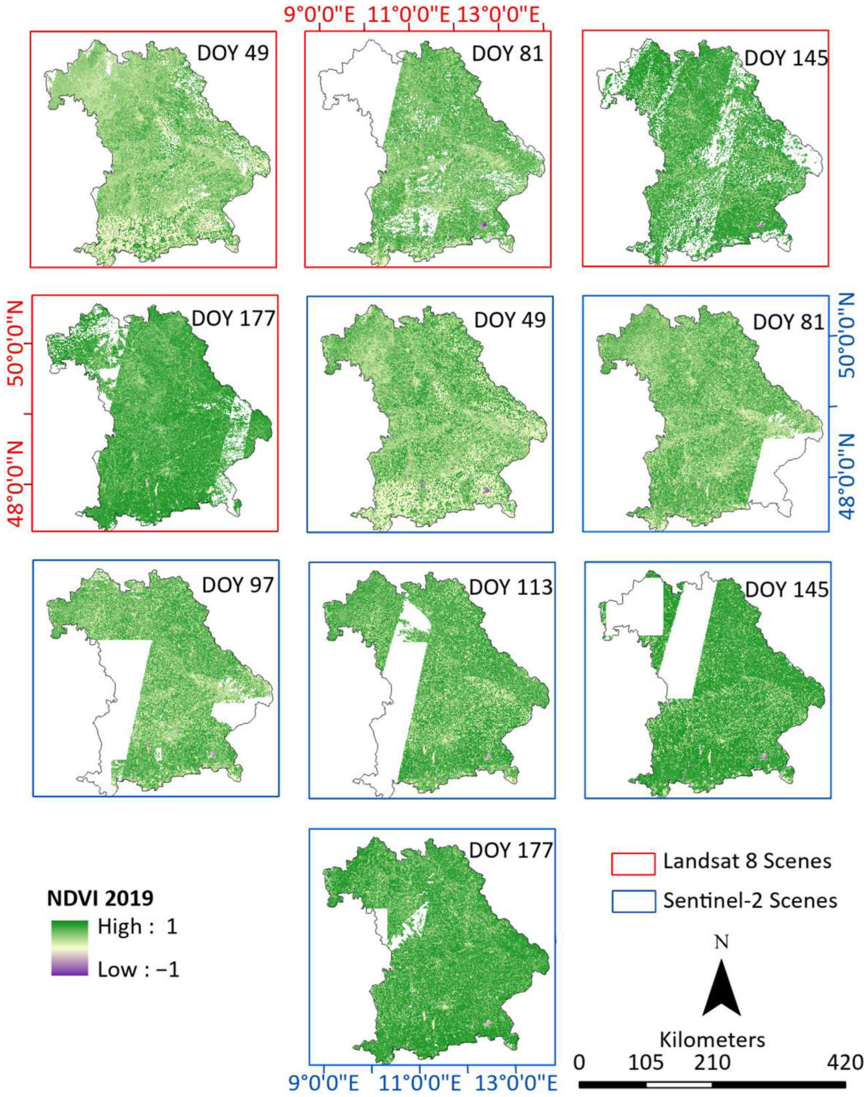
This study employed two freely available spatially high-resolution products obtained from the Sentinel-2 Copernicus program and Landsat 8 Land Surface Reflectance Code (LASRC). The LASRC Tier 1 offers seven spectral bands (coastal/aerosol, blue, green, red, near-infrared (NIR), shortwave infrared (SWIR) 1, SWIR 2) with a spatial resolution of 30 m on a Universal Transverse Mercator (UTM) projection. Using the snow, shadow, and cloud masks, the created C function of the mask (CFMask) method removed snow (Bit 4), clouds (Bit 5), and cloud shadows (Bit 3) using the “pixel_qa” band. After preprocessing, the available snow-free, cloud-free, and shadow-free Landsat images were acquired in 2019 for the state of Bavaria on the following day-of-year (DOY), respectively: 49 (18 February), 81 (22 March), 145 (25 May), and 177 (26 June) (Figure 3).
Moreover, this study also used Sentinel-2 data, which enabled global coverage, five-day return frequency, and multi-spectral imaging with 12 spectral bands at spatial resolutions of 10–20 m. Sentinel-2’s surface reflectance data were processed using the Google Earth Engine after being acquired from the Copernicus Open Access Hub (accessed on 2 August 2021) [51]. The data were computed using sen2cor, which used three quality assessment (QA) bands to create cloud-free images with a QA60 bitmask band containing cloud mask information. After preprocessing, the available Sentinel-2 images were acquired in 2019 for the state of Bavaria at the following DOY, respectively: 49 (18 February), 81 (22 March), 97 (7 April), 113 (23 April), 145 (25 May), and 177 (26 June) (Figure 3).
For data fusion, the coarse resolution MOD13Q1 V6 product was used in this study to generate L-MOD13Q1 and S-MOD13Q1 by fusing it with the preprocessed Landsat and Sentinel-2 data. MOD13Q1 provided an NDVI value per pixel with 250 m spatial and 16-day temporal resolution. In the composed product of MOD13Q1, the NDVI value of a pixel value is assigned with the minor rules and best viewing geometry to the first date of a 16-day time frame. Pixels with constraints (e.g., shadows, clouds) were masked using the quality information (QA) provided along with the NDVI band. Considering the day of acquisition and the QA, linear interpolation of all NDVI values was performed on the product [52] to generate a time series without gaps.
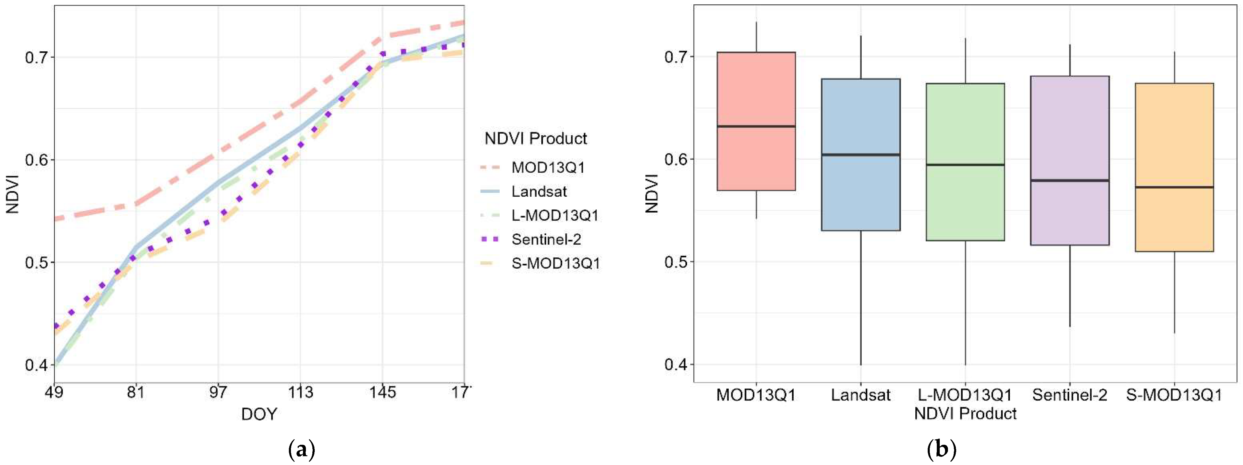
The present study used the synthetic L-MOD13Q1 (30 m, 16 days) and S-MOD13Q1 (10 m, 16 days) NDVI time series generated by [4] as input to the two CGMs obtaining crop yields. Both synthetic products (16 days), L-MOD13Q1 and S-MOD13Q1, were generated using the STARFM and the 8-day products were further developed by applying the linear interpolation approach on 16-day products. The 8- and 16-day time series for RS products were obtained for DOYs from the stem elongation phases until the flowering stages of both WW and OSR. For OSR, the start of the season was 15 February and the end of the season was 20 April 2019 [53]. Moreover, for WW, the start- and end-of-the-season period lay between 15 April and 30 June 2019 [54]. In addition, MOD13Q1 (i.e., just the MODIS NDVI time series without image fusion) was also chosen as an input to the CGMs to allow a comparison between the synthetic and the raw RS time series for crop yield estimation. Based on our previous study, the accuracy assessments of STARFM-generated L-MOD13Q1 and S-MOD13Q1 NDVI products (further used as input for the two CGMs) with the real Landsat and Sentinel-2 NDVI for the agricultural LC class are shown in Table 2 [4]. Our previous study briefly discussed the accuracy assessment of different spatial, temporal products [4]. However, the present study also evaluated synthetic NDVI products’ performance by comparing them with the real NDVI products of Landsat, Sentinel-2, and MOD13Q1. This study compared the mean NDVI values for all RS products used by taking 10,000 random points in Bavaria.

2.2.2. Climate Data

The climate data for 2019 with a daily temporal resolution includes variables such as maximum, minimum, and dewpoint temperature, solar radiation, sunshine hours, precipitation, soil moisture, solar radiation, evaporation, and transpiration. This information was obtained by dynamical downscaling the ERA5 reanalysis dataset, provided by the European Centre for Medium-Range Weather Forecasts [55], to a horizontal grid resolution of 2 km using the hydrologically enhanced Weather Research and Forecasting model [56,57]. A more detailed description of the chosen downscaling approach is provided by [58] and [59]. For this study, the daily climate data are aggregated into 8- and 16-day temporal periods and adapted to the CGMs. Like the satellite data, the present study considers the 8-day climate data for the same SOS and EOS for WW and OSR as described in Section 2.2.1.

2.2.3. InVeKos Data

The field-based InVeKos data are used to identify the fields of WW and OSR in 2019 country-wide. InVeKos data are collected through the Integrated Administration Control System (IACS) (www.ec.europa.eu/info/index_en, accessed on 21 June 2021), which is available for all agricultural plots in European Union (EU) countries by allowing farmers to indicate their agricultural areas graphically. In the IACS, European Union countries are responsible for the administration and control of payments to farmers through a principle called shared management.

2.2.4. LfStat Data

The Bayerisches Landesamt für Statistik (LfStat) is the crop yield validation data providing the crop yield information of 29 crop categories, including WW and OSR in Bavaria on a district level in 2019 (source: www.statistikdaten.bayern.de/genesis/online/, Statistics Code: 41241, accessed on 21 June 2021). The LfStat data were used to validate the LUE-modelled yields of WW and OSR. The validation results were used to check the model’s accuracy, consistency, and stability in generating the yield results in the region. The validation was limited to the rural areas, with the city districts excluded (Figure A1).

2.3. Method

2.3.1. WOFOST

The WOFOST model is a process-based mechanistic model that describes crop parameters such as crop biomass and yield by considering crop genetic properties and climatic and management parameters [60]. The significant processes are CO2 assimilation, transpiration, respiration, phenological development, and dry matter formation (crop biomass). The model states crop biomass as a function of solar radiation, temperature, and daily crop characteristics. LAI is a vital state variable in the WOFOST model to analyse dynamic growth processes. The model simulates the daily crop growth rate, the gross CO2 assimilation rate that depends on the LAI, and incoming radiation. In addition, LAI is an essential parameter for the calculation of the potential transpiration in the model. The inputted LAI is calculated as a function of NDVI for WW and OSR (Table 3).
The daily gross assimilation rate of the crop is calculated by the daily absorbed radiation and the photosynthetic characteristics of each leaf, and it further calculates the total carbohydrates (CH2O) produced. Some fractions of the CH2O produced are used to provide energy for respiration (maintenance respiration), with the remaining energy converted into dry matter. The model calculates the growth rate as:
G = C e ( A R m )
where ∆G is the growth rate (kg dry matter ha−1 d−1), A is the gross assimilation rate (kg CH2O ha−1 d−1), Rm is the maintenance respiration rate (kg CH2O ha−1 d−1), and Ce is the conversion efficiency (kg dry matter kg−1 CH2O). Based on Monteith’s Principle of Light Use Efficiency, the calculation of total dry matter (kg dry matter ha−1 yr−1) in the WOFOST model is equivalent to the net primary production (NPP) (kg ha−1 yr−1) [20,63].
This study adopted the complete working methodology of this model from the WOFOST 6.0 documentation prepared by [64], which is also available online (www.wur.nl). The complete calculation, with input parameters to calculate the growth of a WW and a OSR biomass, makes the WOFOST model complex in design. The conceptual diagram of the complete WOFOST model is shown in Figure A2. The WOFOST model is calibrated using the values given in Table 4.

2.3.2. LUE

The LUE model is based on a Light Use Efficiency principle [20,21] and is coupled with the RS data using a similar methodology [5,65]. The model is based on a semi-empirical approach and calculates the FPAR [66] and the daily aboveground biomass as:
B i o m a s s = P A R F P A R
F P A R = 1.222 N D V I + 0.1914
= T m i n m i n V P D K s o
where PAR is photosynthetically active radiation (MJ m−2 d−1), FPAR is the fraction of PAR absorbed by the canopy, ∈ is the actual Light Use Efficiency (g C M J−1), ∈o is the actual Light Use Efficiency (g C M J−1), Tminmin′ is the minimum of the minimum temperature (°C) index, VPD is the vapour pressure deficit (kPa) index, and Ks is the soil moisture stress index. The temperature and vapour pressure indexes are calculated using the minimum and maximum values for the study region. The total aboveground biomass calculated by the LUE model is equivalent to the net primary productivity (NPP) (kg ha−1 yr−1). A brief explanation of the model with a flow diagram is described in our previous study [5]. The specific model is not only selected for its performance but also its high processing speed and low requirement of input parameters compared to the other CGMs. The linear regression equations used to calculate crop yields of WW and OSR for different satellite biomass products using LUE are shown in Table A1.
Both models (LUE and WOFOST) were calibrated by using values shown in Table 4. This study used a minimum lethal temperature of −2 °C for WW and OSR [67,68,69]. In the other studies, the optimal minimum values of temperature of WW and OSR at growth stages were 10 °C and 12 °C, respectively [67,68,69]. For the Vapor Pressure Deficit (VPD), the present study followed [70], which analysed the environmental impact on leaf gas exchange of WW with minimum and maximum values of 1.5 and 4.0 kPa, respectively. The value used for optimal Light Use Efficiency was 3 gC/MJ [71].
Table 4. Description of model calibration values taken from the related literature for the WOFOST and LUE models, plus, the climate thresholds used to calculate the climate stress indexes used in the design of a model.
ParameterDescriptionModel(s)ValueUnitsReference
ξScattering coefficientWOFOST0.2-[60]
kdfDiffusion coefficientWOFOST0.72-[72]
AmGross assimilation rateWOFOST4g/m2[73]
CeConversion coefficientWOFOST0.0399-[74]
oLight use efficiencyWOFOST&LUE3gC/MJ[71]
Tmin minMinimum of minimum temperatureWOFOST&LUE−2°C[67]
Tmin maxMaximum of minimum temperatureWOFOST&LUE12°C[70]
VPD minMinimum VPDLUE1.3–1.5k Pa[75,76]
VPD maxMaximum VPDLUE3.6–4k Pa[75,76]
ZrMaximum root depthWOFOST&LUE1.5–1.8m[77]
PAverage fraction of TAWWOFOST&LUE0.55-[77]

2.3.3. Sensitivity Analysis

This study performed a sensitivity analysis of the LUE and WOFOST models for both WW and OSR in Bavaria in 2019. The values of climate variables were optimised in the design of every model. During the analysis, the impact of climate stress factors was nullified, and the biomass calculation replaced the actual Light Use Efficiency (ε) values with the optimal (εo) values.

2.3.4. Statistical Analysis

Both the referenced and the modelled (LUE and WOFOST) crop yields of WW and OSR were validated using LfStat crop yield (with a 95% confidence interval) for 2019, respectively. The quality (R2) and the precision (root mean square error (RMSE)) of the obtained results were calculated using a linear regression model (LRM), which aimed to establish a linear relationship between the referenced (independent variable) and modelled yields (dependent variable) of WW and OSR at different spatial (10, 30, and 250 m) and temporal (8 and 16 days) scales. The statistical parameters used to validate and compare the accuracies of the LUE- and WOFOST-modelled yields with the referenced yield are R2 (Equation (5)), Mean Error (ME) (Equation (6)), RMSE (Equation (7), and relative RMSE (RRMSE) (Equation (8)). To compare the yield outputs of both models, this study considered RRMSE < 15% as good agreement, 15–30% as moderate agreement, and > 30% as poor agreement [78]. The lower the value of ME, RMSE, and RRMSE, the better the model performed.
R 2 = ( ( P i P ) ( O i O ) ) 2 ( P i P ) ) 2 ( O i O ) ) 2 ,
M E = 1 n i = 1 n O i P i 2
R M S E = M E ,
R R M S E ( % ) = R M S E 1 n i = 1 n O i 100 ,
where Pi is the predicted value, Oi is the observed value, P’ is the predicted mean, O’ is the observed mean value, n is the total number of observations, referenced yieldy is the LfStat yield of every district in 2019, and modelled yieldy is the LUE-generated yield of every district in 2019. The results’ significance was obtained by observing the probability value (p-value) calculated using the LRM with a H0 that no correlation exists between the referenced and the modelled or synthetic values and an H1 that the correlation exists. The test was performed at a significance (or alpha (α)) of 0.05. A p-value lower than 0.05 indicates that the model is significant and rejects the H0 that there is no correlation.

3. Results

3.1. Evaluation of Real (MOD13Q1, Landsat, and Sentinel-2) and Synthetic (L-MOD13Q1 and S-MOD13Q1) Satellite NDVI Products

The spatial visualisation of the products MOD13Q1, Landsat, L-MOD13Q1, Sentinel-2, and S-MOD13Q1 at DOY 145 is shown in Figure 4, respectively. Both synthetic products, L-MOD13Q1 and S-MOD13Q1, had shown higher dependency on their high-resolution products (Landsat and Sentinel-2) than MOD13Q1. Figure 4f shows the spatial location of 10,000 random points that compares real and synthetic NDVI products with their respective low pair (MOD13Q1) and high pair (Landsat or Sentinel-2) products by considering the mean values at different DOYs (Figure 5). Figure 5a,b show the line and box plot comparison of real and synthetic products and their interquartile comparison of NDVI values.
Both synthetic products underestimated the NDVI values compared to their actual NDVI products between DOYs 81 and 145 (Figure 5a). From DOYs 145 to 177, Landsat, L-MOD13Q1, Sentinel-2, and S-MOD13Q1 achieved a mean NDVI of approx. 0.71. The median NDVI values of L-MOD13Q1 and S-MOD12Q1 lie close to their respective high pair product (Figure 5b).

3.2. Statistical Analysis of Crop Yields Obtained from LUE and WOFOST Models for WW and OSR Using Multisource Data in 2019

Both 8- and 16-day NDVI inputs, such as L-MOD13Q1 and S-MOD13Q1 and MOD13Q1, performed significantly for WW and OSR with LUE and WOFOST models (p-value < 0.05); this rejects the H0 of the LRM that there is no relationship between the modelled and measured crop yield (Figure 6 and Figure 7). The linear regression equations obtained to calculate crop yields of WW and OSR for different satellite biomass products with both models are shown in Table A1. The R2 values obtained from the S-MOD13Q1 NDVI (8 and 16 days) products have a higher accuracy compared to the L-MOD13Q1 (8 and 16 days) and MOD13Q1 (8 and 16 days). Based on the R2 of the different spatial resolutions of the NDVI products for WW, the models’ descending order is LUE (S-MOD13Q1, 10 m, 8 days), LUE (S-MOD13Q1, 10 m, 16 days), LUE (L-MOD13Q1, 30 m, 8 days), LUE (L-MOD13Q1, 30 m, 16 days), WOFOST (S-MOD13Q1, 10 m, 8 days), WOFOST (L-MOD13Q1, 10 m, 8 days), LUE (MOD13Q1, 250 m, 8 days), WOFOST (S-MOD13Q1, 10 m, 16 days), WOFOST (MOD13Q1, 250 m, 8 days), WOFOST (MOD13Q1, 250 m, 16 days), WOFOST (L-MOD13Q1, 30 m, 16 days), and LUE (MOD13Q1, 250 m, 16 days), with R2 values of 0.85, 0.85, 0.82, 0.78, 0.78, 0.75, 0.73, 0.73, 0.69, 0.65, 0.64, and 0.52, respectively. In general, the predicted values by both models with different satellite inputs follow a similar pattern, and none of the models can claim to outclass the others. However, the ME and RMSE values give a complete picture of the model comparisons (8-and 16-day products) and performances (i.e., their quality and precision) with every satellite input. The ME and RMSE of WW from the WOFOST (MOD13Q1 8-day) is slightly lower than the WOFOST (L-MOD13Q1 16-day and S-MOD13Q1 16-day); moreover, the RMSE of the WOFOST (S-MOD13Q1 and L-MOD13Q1 (8-day)) is lower than the WOFOST (MOD13Q1 16-day). The overall results of LUE inputting L-MOD13Q1, S-MOD13Q1, and MOD13Q1 8-to-16-days NDVIs range from 5.46 to 6.32 dt/ha (RMSE), 5.01 to 5.40 dt/ha, and 6.52 to 9.33 dt/ha.
Like WW, the R2 of the different spatial resolutions of NDVI satellite products for OSR in descending order are LUE (S-MOD13Q1, 10 m, 8 days), LUE (L-MOD13Q1, 30 m, 8 days), LUE (S-MOD13Q1, 10 m, 16 days), LUE (L-MOD13Q1, 30 m, 16 days), LUE (MOD13Q1, 250 m, 8 days), WOFOST (S-MOD13Q1, 10 m, 8 days), WOFOST (L-MOD13Q1, 10 m, 8 days), LUE (MOD13Q1, 250 m, 16 days), WOFOST (S-MOD13Q1, 10 m, 16 days), WOFOST (L-MOD13Q1, 30 m, 16 days), WOFOST (MOD13Q1, 250 m, 8 days), and WOFOST (MOD13Q1, 250 m, 16 days), with R2 values of 0.82, 0.80, 0.80, 0.78, 0.67, 0.64, 0.63, 0.63, 0.63, 0.62, 0.62, and 0.60, respectively. It showed that the LUE model is more accurate at different spatial scales than the WOFOST model. Moreover, the model resulted in higher accuracy for the 8-day products of S-MOD13Q1 and L-MOD13Q1 compared to their 16-day products. The overall results of LUE combining L-MOD13Q1, S-MOD13Q1, and MOD13Q1 8-to-16-days NDVIs range from 2.23 to 2.36 dt/ha (RMSE), 2.11 to 2.39 dt/ha, and 3.02 to 3.40 dt/ha.
For the LUE model for WW, both 8-day products of S-MOD13Q1 (median yield = 71.68 dt/ha) and L-MOD13Q1 (74.65 dt/ha) obtained their yield close to the referenced yield (72.30 dt/ha) (Figure 8). For the LUE model of OSR, the 8-day and 16-day S-MOD13Q1 and L-MOD13Q1 resulted in similar predictions, respectively, where the 8-days (median yield ~33 dt/ha) show the median yield closer to the referenced yield (33.50 dt/ha) than the 16-days (~34 dt/ha) (Figure 8).
Figure 9a,b displayed that the fused products obtained higher R2 and lower RMSE values than the non-fused products for WW and OSR. For example, L- and S-MOD13Q1 resulted in an R2 = 0.72 and 0.76 and RMSE = 4.91 and 4.49 dt/ha, respectively, and MOD13Q1 resulted in an R2 = 0.63 and RMSE = 5.85 dt/ha. Analysing the different temporal resolutions of 8- and 16-day products with LUE and WOFOST models, the 8-day products (median R2 = 0.77, RMSE= 6.14 dt/ha) resulted in higher R2 and lower RMSE than the 16-day products (median R2 = 0.69, RMSE= 8.0 dt/ha) (Figure 9c,d).

3.3. Spatial Analysis of Crop Yields Obtained from LUE and WOFOST Models for WW and OSR Using Multisource Data in 2019

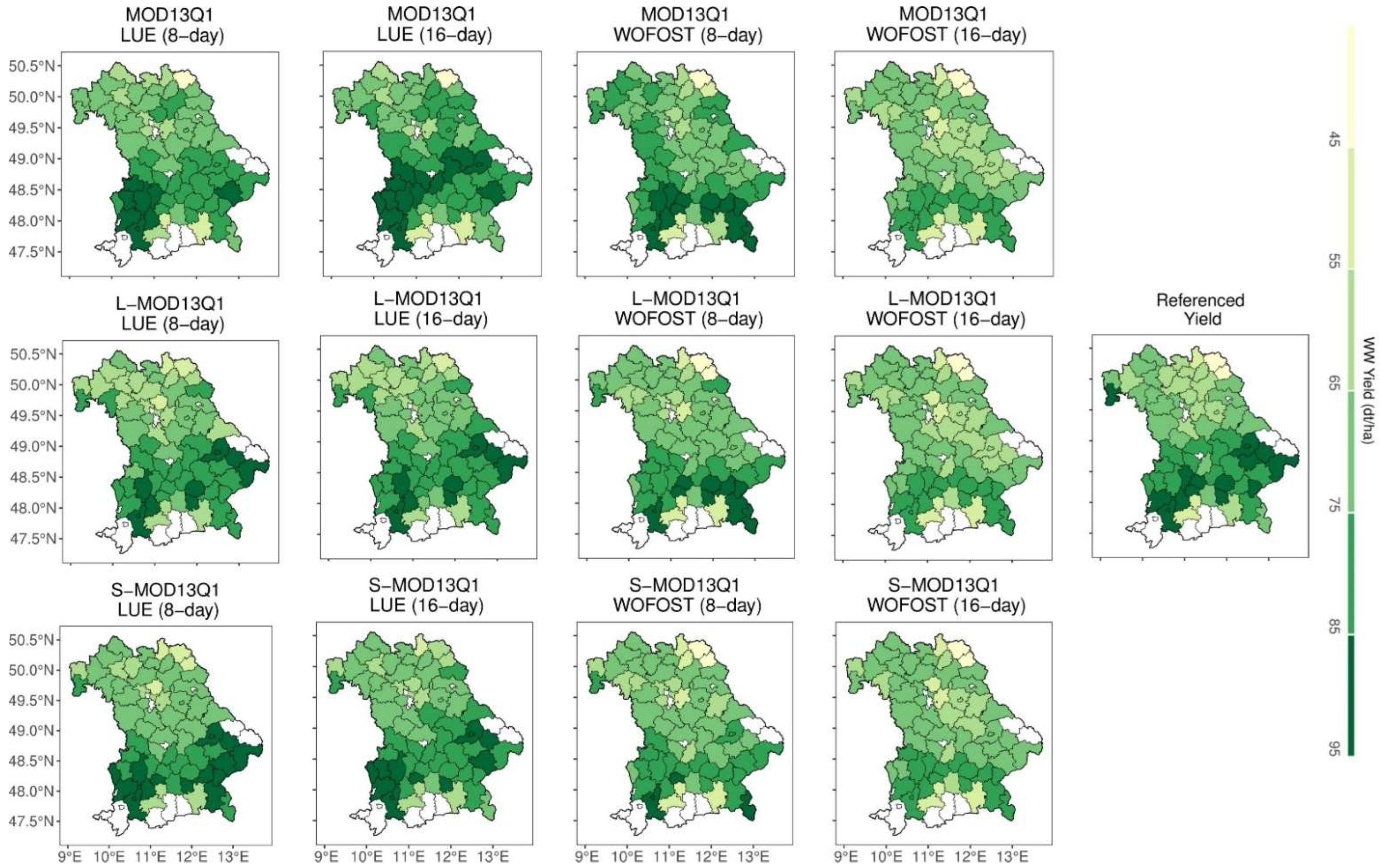
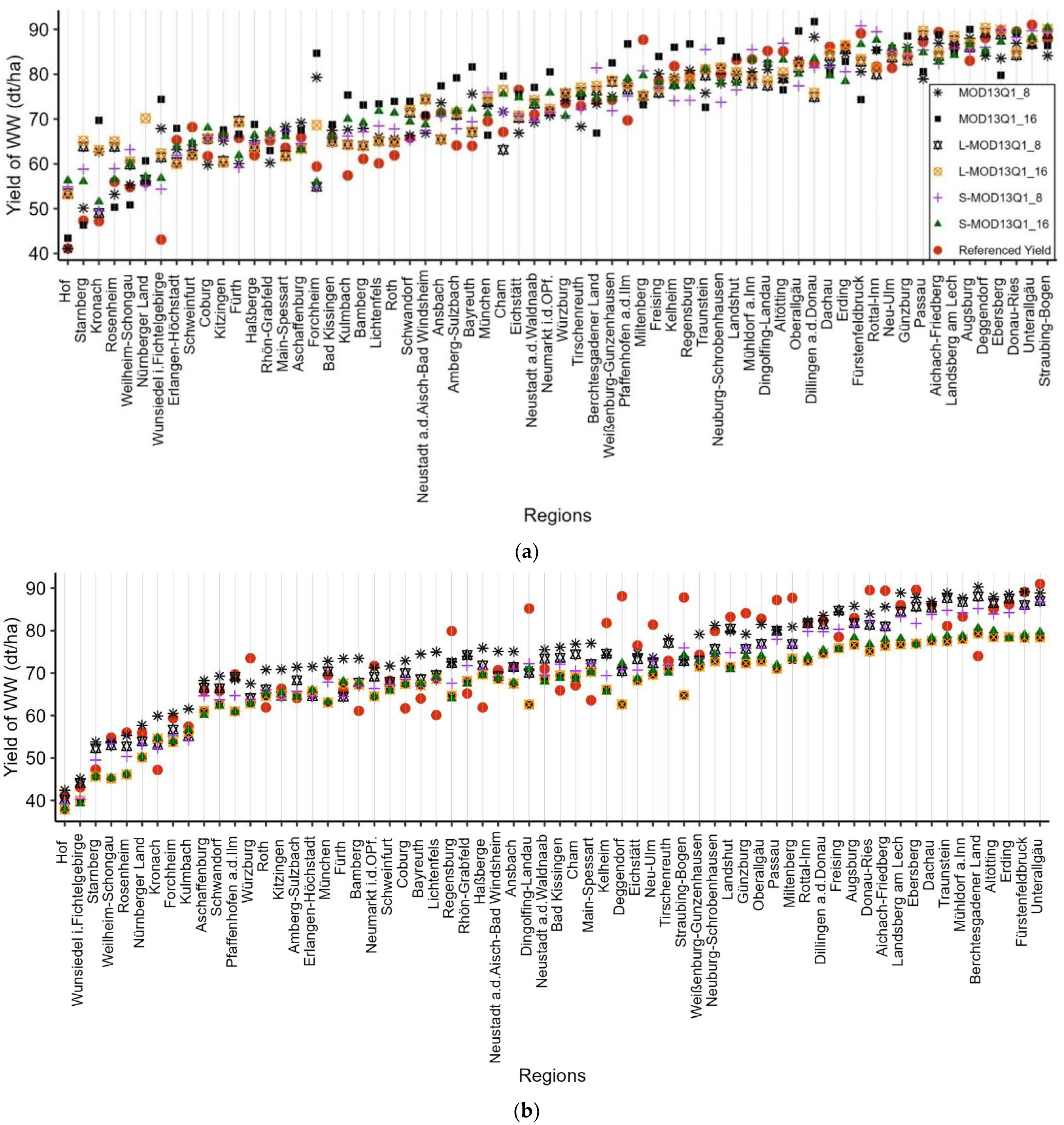
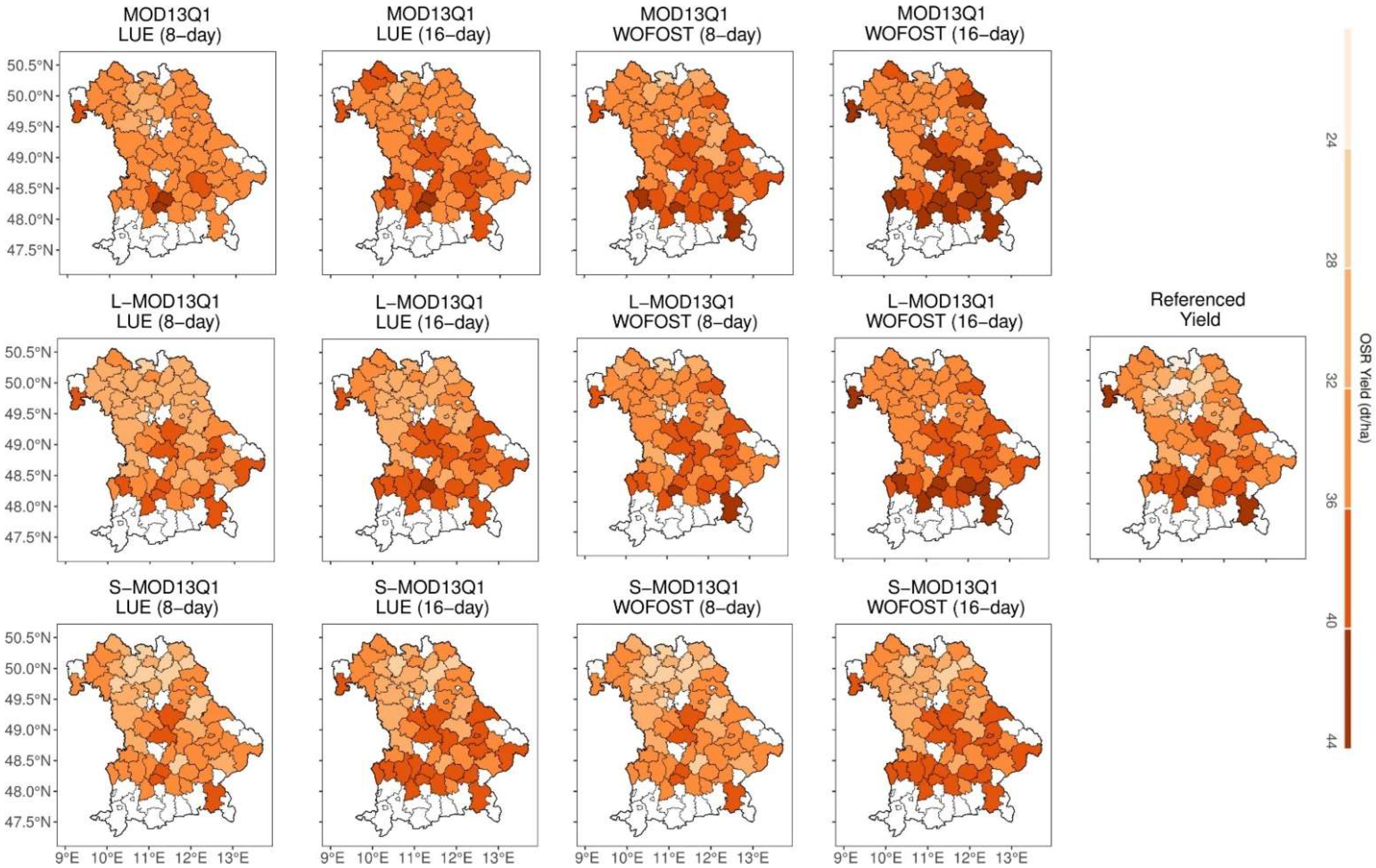
The spatial comparison of crop yield at the regional level from the referenced and modelled yields with multi-source data was displayed for both WW and OSR (Figure 10, Figure 11, Figure 12 and Figure 13). For WW, the LUE model showed consistency in yield prediction for regions such as Straubing-Bogen, Bad Kissingen, Landsberg am Lech, Dillingen a.d. Donau, Fresing, Würzburg, Neuburg-Schrobenhausen, Fürth, Neustadt a.d. Aisch, Bad Windsheim, Rhön-Grabfeld, Oberallgäu, Regensburg, Aschaffenburg, and Ansbach for all satellite inputs. However, the WOFOST model showed stability for regions such as Freising, Tirschenreuth, Neustadt a.d. Waldnaab, Kitzingen, Fürth, Schweinfurt, Weißenburg-Gunzenhausen, Neustadt a.d. Aisch-Bad Windsheim, and Kulmbach. The S-MOD13Q1 8-day showed higher spatial accuracy than other remote sensing inputs used in both models. The S-MOD13Q1 8-day product with LUE predicted a higher yield of more than 85 dt/ha for regions such as Altötting, Passau, Straubing-Bogen, Deggendorf, Fürstenfeldbruck, Donau-Ries, Ebersberg, and Unterallgäu, like the referenced yield (Figure 11a). However, when inputted into the WOFOST model, the exact product underestimated the yield for all regions (except Fürstenfeldbruck and Unterallgäu) (Figure 11b).
Similarly, for the OSR, both models showed consistency in yield prediction in regions such as Ebersberg, Eichstätt, Lichtenfels, Würzburg, Roth, Schweinfurt, Dingolfing-Landau, Neustadt a.d. Waldnaab, Pfaffenhofen a.d. Ilm, Kelheim, and Mühldorf a.Inn for all satellite inputs (Figure 12). The WOFOST model had overestimated the crop yields with MOD13Q1 (8 and 16 days) for nearly 18 regions (>40 dt/ha) compared to the referenced yield (Figure 13a,b). The L-MOD13Q1 8-day resulted in an overestimation of crop yields compared to the L-MOD13Q1 8-day product with both LUE and WOFOST models.

3.4. Sensitivity Analysis

The sensitivity analysis compared the models’ (LUE and WOFOST) performance by excluding the effect of climate stress factors for both WW and OSR in Bavaria in 2019. The LUE- and WOFOST-modelled yields showed a higher correlation with the referenced yield when the climate stress factors were included and vice versa. Both models showed higher R2 and lower RMSE values compared with the yield values obtained during the sensitivity analysis (Figure 14). The overall accuracies obtained during the sensitivity analysis of both LUE and WOFOST were recorded as R2 of 0.61 and 0.58 and RMSE of 6.13 dt/ha and 6.32 dt/ha, respectively (Figure 14). Including climate parameters improved both models’ performance, reducing the RMSE by −38% (LUE) and −11% (WOFOST) and increasing the R2 from 19% to 12%, respectively.

3.5. Suitable Crop Growth Model

The statistical analysis showed the R2, RMSE, RRMSE, and ME values of the model’s (LUE and WOFOST) performance, including climate stress factors’ effect on both WW and OSR in Bavaria in 2019 (Figure 15). The LUE model resulted in a higher R2 (>0.78) for the 8- and 16-day products of L-MOD13Q1 and S-MOD13Q1 than the WOFOST model (R2 < 0.71). Similarly, the RMSE and ME of these products show more accurate results with the LUE model (RMSE <4.5 dt/ha, ME <3.3 dt/ha) than the WOFOST model (RMSE < 7.0 dt/ha, ME < 6.0 dt/ha). MOD13Q1 8-day (R2 < 0.66, RMSE < 5.19 dt/ha, ME < 4.03 dt/ha) achieved higher accuracy than MOD13Q1 16-day (R2 < 0.62, RMSE < 7.10 dt/ha, ME < 5.86 dt/ha) with both LUE and WOFOST. The RRMSE for both models show better agreement (<15%) between the observed and modelled yields for all satellite products. However, the LUE model (<11.50%) showed an overall lower RRMSE than the WOFOST model (<13.67%) at different spatial and temporal scales. Irrespective of the crop type and satellite spatial scale, the LUE model obtained higher R2 and lower RRMSE (average R2 = 0.77, RRMSE = 8.17 %) than the WOFOST model (average R2 = 0.66, RRMSE = 11.35%) (Figure 16).

3.6. Visualisation of the Modelled Crop Biomass by the LUE Model in 2019

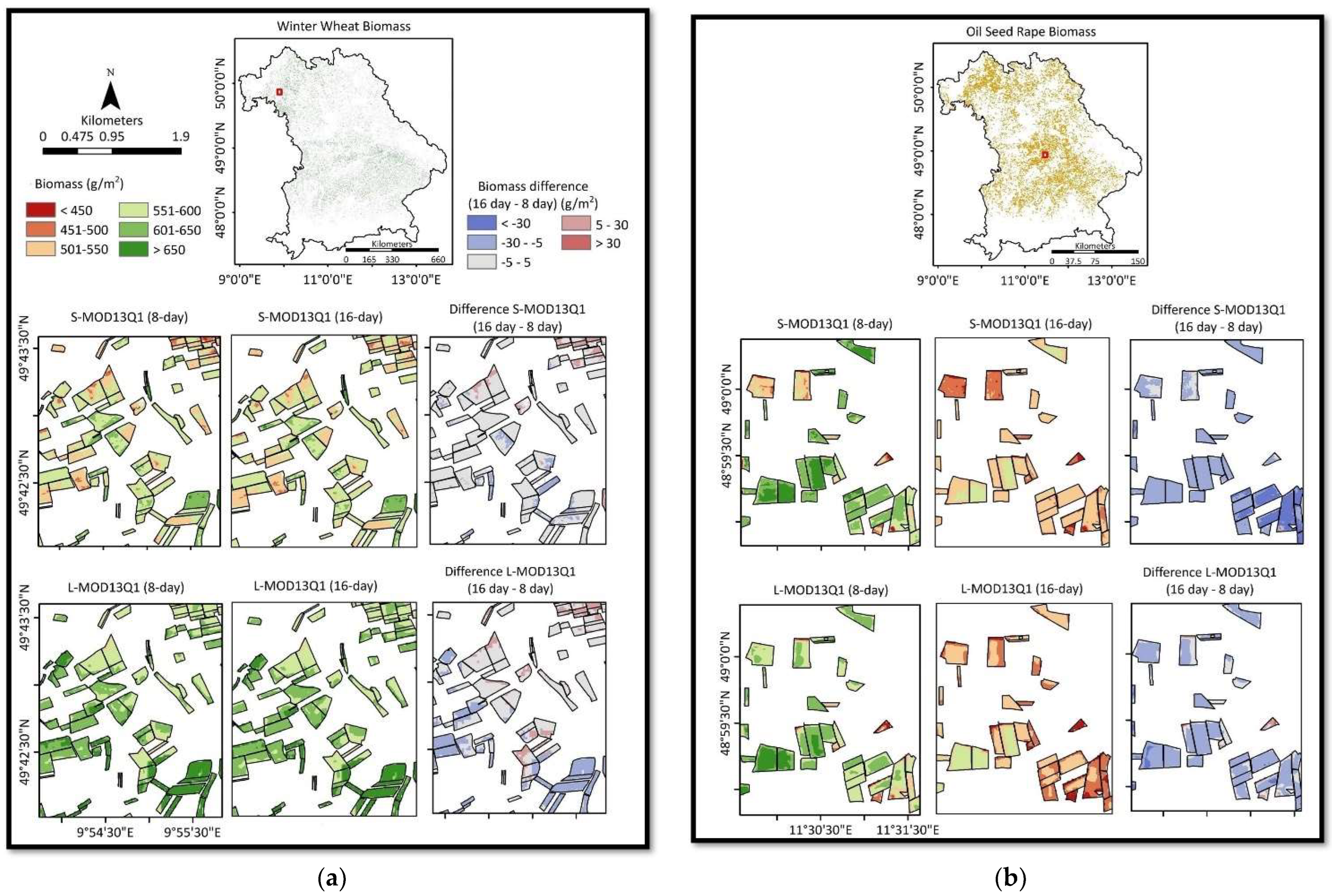
Figure 17 shows the spatial distribution of simulated crop biomass for WW and OSR by the LUE model at 10 and 30 m spatial resolutions with 8- and 16-day temporal resolution for Sentinel-2 (S-MOD13Q1) and Landsat (L-MOD13Q1), respectively. The field-based biomass OSR and WW biomass values vary between 771.36 and 1112.58 g/m2, respectively. These values were obtained considering the climate stress factors, such as temperature, VPD, and soil moisture stress. Every figure shows the difference between the 8-day and 16-day biomass products. The difference in 8- and 16-day WW products varies between −72.57 g/m2 and 80.50 g/m2, respectively. The results indicate that for WW, S-MOD13Q1 had almost similar results at both temporal resolutions; however, a slight variation in L-MOD13Q1 was seen. For OSR, a little difference in the field-based biomass was observed in both 8- and 16-day products of Sentinel-2 and Landsat. The 8-day products in WW and OSR for L-MOD13Q1 and S-MOD13Q1 showed an overestimation in crop biomass compared to the 16-day products.

4. Discussion

This study finds the RS data’s optimal spatial and temporal resolutions combined with CGMs for accurate crop yield predictions for Bavaria in 2019. The results are obtained using WOFOST (complex model) and LUE (simple model) CGMs by individually inputting them with climate variables plus six different remote sensing products (Real: MOD13Q1 (250 m), Synthetic: L-MOD13Q1 (30 m) and S-MOD13Q1 (10 m)) at 8 or 16 days of temporal resolution. This study investigates the significance of the more straightforward, more accurate, and faster LUE model with less input requirement than the complex WOFOST model with a high demand of climatic input variables. The sensitivity analysis is performed to obtain the influence of climate stress factors on crop yield predictions with different satellite inputs. The following sections provide a brief discussion of the points mentioned above.

4.1. Importance of the Synthetic Data in Crop Yield Modelling

Many studies employing satellite images aimed to compensate for the gaps in the primary data by fusing data with another source for various remote sensing applications [4,5,10,79]. The data fusion is to increase the spatial resolution of the relatively coarse images collected by satellites with high revisit frequencies. The fused results usually inherit the details of the high spatial resolution images and the temporal revisit of the frequencies of their counterparts [79]. In the past two decades, data fusion techniques such as the STARFM and its variants have been applied to satellite images for different applications, including phenology analysis [80,81,82], yield and drought monitoring [83,84,85], forest mapping [46,86], and biophysical parameter estimation [85,87,88,89]. Landsat and MODIS images dominate data fusion; however, other satellite combinations, such as Sentinel-2, Sentinel-1, or Worldview, are being increasingly adopted. However, despite its advantages, the data fusion technique could have challenges. For example, combining different sensors could result in misalignment and inaccuracy. In addition, lower sensor quality in data fusion can affect the results’ accuracy [90]. Therefore, to analyse the quality of data fusion products, this study evaluated the significance of real and synthetic NDVI products by considering the mean NDVI of 10,000 randomly selected points and comparing their mean values at different DOYs. For both L-MOD13Q1 and S-MOD13Q1, the mean values obtained lie close to their respective high-resolution product. Therefore, the accuracy of these products is higher. It leads this study to investigate the potential of synthetic products in crop yield modelling.
Moreover, to further improve the data quality and reduce the computation cost of data fusion, this research employs the “index-then-blend” (IB) technique, which creates the NDVI from both the high pair and low pair images before blending them for data fusion [50]. The results of a preliminary study [23] also indicate that the STARFM could successfully fuse MODIS (MOD13Q1, 250 m, 16 days) with Landsat (output: L-MOD13Q1, 30 m, 16 days) and Sentinel-2 (output: S-MOD13Q1, 10 m, 5–6 days) imagery using the above approach [4,5,91,92]. The low RMSE and high R2 obtained for the agricultural class with both L-MOD13Q1 (R2 = 0.60, RMSE = 0.11) and S-MOD13Q1 (R2 = 0.68, RMSE = 0.13) through the STARFM are comparable to those obtained by other studies [20,39,40,87]. One of our previous studies stated the high potential of data fusion between Landsat and MCD43A4 MODIS products on achieving an R2 of 0.61 and RMSE of 0.10 for WW biomass monitoring at Mecklenburg–West Pomerania in Germany [5]. The higher correlations between the observed and predicted NDVI values indicate the suitability of the algorithm for vegetation monitoring. Other studies with spatiotemporal data fusion have used NDVI as their primary input for applications such as crop biomass and yield monitoring [80,81,82,83,84,85,87,88,89]. The present study highlights the importance of the synthetic NDVI time series in crop yield modelling by analysing the accuracy assessment between the raw satellite imagery MOD13Q1 (without fusion) and L and S-MOD13Q1 (with fusion). The crop yield prediction results conclude the need for data fusion (obtaining high-resolution satellite data) for accurate crop yield prediction. Many studies demonstrated the potential of high spatial and temporal remote sensing data to describe the spatiotemporal variability of crop biophysical parameters [93], where the availability of Landsat and Sentinel-2 images offer new perspectives for crop monitoring and modelling.
This study obtains higher crop yield accuracy with the fused products (L- and S-MOD13Q1: R2 = 0.72 and 0.76 and RMSE = 4.91 and 4.49 dt/ha) than the non-fused product (MOD13Q1: R2 = 0.63 and RMSE = 5.85 dt/ha) for both WW and OSR irrespective of the crop model (LUE or WOFOST) (Figure 9a,b). While comparing the yield prediction accuracies of both fused products, S-MOD13Q1 results are more accurate than the L-MOD13Q1. Due to its higher temporal frequency, Sentinel-2 (5–6 days) had six cloud-free scenes (DOYs: 49, 81, 97, 113, 145, and 177) than the Landsat (16 days), with only four cloud-free scenes (DOYs: 49, 81, 145, and 177) available for the analysis (Figure 2). Due to this lower gap in Sentinel-2 DOYs, the NDVI-fused product (S-MOD13Q1) results in higher accuracy than the Landsat-based product (L-MOD13Q1) [4], which further improves the crop yield prediction accuracy of the former more than the latter. However, the L-MOD13Q1 product is still advantageous for generating and exploring the long-term yield time series due to the availability of Landsat data since 1982 with a maximum resolution of 30 m [10].
Results from previous studies have also shown that the assimilation of RS with high spatial-temporal resolution can significantly improve the accuracy of the output, e.g., with an R2 value of 0.86 for the LAI measurements using Sentinel-2 as shown by [94]. Dhillon et al. [5] measured the accuracy of LUE with MODIS and the STARFM; both proved to be more reliable and significant with high R2 (>0.64, >0.82) and low RMSE (<650 g/m2, <600 g/m2), where MODIS resulted in lower accuracy due its coarser resolution. Further, Huang et al. [95] found that the low spatial resolution of MODIS degrades the output accuracy in crop modelling up to 60%.
The high temporal resolution data help to improve a crop’s accuracy by covering the complete crop stages and measuring climate variables’ impact. The lower the temporal gaps, the higher the attainable accuracies by the crop models [96]. The present study shows that the 8-day products are more accurate for yield prediction than the 16-day products. The 8-day products are more likely to cover fine details of the crop physiology, resulting in higher accuracy. Analysing the different temporal resolutions of 8- and 16-day products with LUE and WOFOST models, the 8-day products (median R2 = 0.77, RMSE = 6.14 dt/ha) show a better relationship between the referenced and modelled yields than the 16-day products (median R2 = 0.69, RMSE = 8.0 dt/ha) (Figure 9c,d). Therefore, this study concludes that high spatial and temporal remote sensing products are essential for crop growth monitoring influenced by climatic factors [5,9].
Even though the data fusion products obtained in this study resulted in higher accuracy than the non-fused products, many studies have suggested more improvements in the STARFM algorithm [25,37,40]. For example, [97] discussed the inevitable role of different sensors and image-processing algorithms causing inconsistency in the data.

4.2. Importance of Linking Crop Growth Models with RS in Crop Yield Modelling

Crop yield prediction has been considered significant to food security and sustainable agricultural development [29]. This study merged remotely sensed data with process-oriented crop models, which can yield more accurate estimates of model outputs. It gives our approach an advantage over conventional studies that use CGMs [98,99,100]. The current study used the traditional technique of CGMs to monitor WW and OSR yields of Bavaria by integrating STARFM-generated S-MOD13Q1 (10 m, 8 and 16 days) and L-MOD13Q1 (30 m, 8 and 16 days) and raw MOD13Q1 (240 m, 8 and 16 days) products in the two CGMs: WOFOST and LUE.
The performance of both models is compared based on their complexity in design, processing speed, accuracy, and precision. This study found that the WOFOST model, which requires more input parameters, is complex in its design and needs more computing time to generate the output than the LUE model. Compared to the other CGMs, the LUE model is based on the fundamental principles of photosynthesis, considers each crop’s unique properties, and can be calibrated and validated using RS technology [20,21,101]. The model accounts for the crop’s ability to use solar radiation for photosynthesis by correlating its biomass with the amount of solar radiation it receives [102,103]. By using RS-derived NDVI with the amount of solar radiation the crop is absorbing (i.e., APAR), the LUE model can use these variables for its calibration and validation, which makes it more accurate in predicting crop yields [104,105]. The performance of the LUE model in forecasting crop yields also shows consistency with other studies [5,9,106]. Yuan et al. [103] successfully validated the crop yields using the satellite-based LUE model at 36 crop sites. Similar research effectively used the Light Use Efficiency variable for biomass estimation of WW and maize using the Production Efficiency Model [107]. Comparing the results of LUE obtained by [5], the model resulted in an R2 of 0.83 and RMSE of 581.82 g/m2, which is very close to the results obtained in the present study (R2 = 0.81, RMSE = 5.17 dt/ha). Irrespective of the crop type and satellite spatial scale, the results of this study show that the LUE model (average R2 = 0.77, RMSE = 4.45 dt/ha) performed more accurately than the WOFOST model (average R2 = 0.66, RMSE = 7.75 dt/ha) (Figure 16).
The WOFOST model differs from the LUE model by making the potentially unrealistic assumption that crop growth rates are constant throughout the growing season [108]. For instance, crops may experience periods of stress or damage from pests or diseases, which can affect their growth rate and, ultimately, their yield. It makes the model rely heavily on input data, such as LAI, soil, weather, and management parameters, which may only sometimes be available, and could be the reason for inaccuracies in yield predictions [109]. However, many studies have successfully used the WOFOST model combined with RS-based LAI to predict crop yields accurately and have discussed its potential limitations [110,111]. Similar to this study, a comparison of five different crop growth models was made, where the WOFOST model resulted in an average R2 of 0.77 and RMSE of 651 g/m2, which matches the results of the present study, where the model for WW resulted in an R2 of 0.71 and RMSE of 7.75 dt/ha [5].
Comparing the crop yield at a regional level, the LUE model showed consistency in yield prediction in districts such as Straubing-Bogen, Bad Kissingen, Landsberg am Lech, Dillingen a.d. Donau, Fresing, Würzburg, Neuburg-Schrobenhausen, Fürth, Neustadt a.d. Aisch, Bad Windsheim, Rhön-Grabfeld, Oberallgäu, Regensburg, Aschaffenburg, and Ansbach for all satellite inputs. However, the WOFOST model showed stability for regions such as Freising, Tirschenreuth, Neustadt a.d. Waldnaab, Kitzingen, Fürth, Schweinfurt, Weißenburg-Gunzenhausen, Neustadt a.d. Aisch-Bad Windsheim, and Kulmbach. Both models are uncertain in districts at higher elevations in the south (Bavarian Alps) and east (Bavarian Forest and Fichtel Mountains) of Bavaria for both WW and OSR. The models overestimated the crop yield in regions such as Regen, Freyung-Grafenau, Bad Tölz-Wolfratshausen, and Garmisch-Partenkirchen. The reason could be the complex topography and different climate and management practices of these regions, which have impacted the performance of both models [112,113]. Comparing the two models, the LUE model with S-MOD13Q1 8-day showed higher spatial accuracy than the WOFOST model. Like the referenced yield, the S-MOD13Q1 8-day product with LUE predicted a higher yield of more than 85 dt/ha for regions such as Altötting, Passau, Straubing-Bogen, Deggendorf, Fürstenfeldbruck, Donau-Ries, Ebersberg, and Unterallgäu. However, when inputted into the WOFOST model, the exact product underestimated the yield for all regions (except Fürstenfeldbruck and Unterallgäu). The instability of models at higher elevations could be due to the bad quality of the synthetic NDVI products for specific districts. Like OSR, the WOFOST model overestimated the crop yields with MOD13Q1 (8 and 16 days) for nearly 18 regions by predicting a yield of more than 40dt/ha compared to the referenced yield. S-MOD13Q1 and L-MOD13Q1 8-day performed better when inputted to the LUE model than the WOFOST.
The quality of the synthetic NDVI product might vary for these regions as the districts have no horizontal or vertical overlay of Landsat scenes within the path row, limiting their coverage frequency. Moreover, the continuous cloud cover in some regions of Bavaria could have negatively impacted the yield prediction accuracy of models (Figure 2).

4.3. Sensitivity Analysis

The climate variables have essential contributions impacting the accuracy of crop yield predictions [9,114,115]. This study analyses the impact of climate elements by performing a sensitivity analysis where the LUE and WOFOST models calculate crop yields of WW and OSR without including the climate stress factors in 2019. Having already been influenced by the effect of climate elements, the obtained referenced yield shows poor accuracy with crop model yield results after excluding climate stress factors from both models. This study shows that including climate stress indices improves the performance of both models, reducing the RMSE by −38% (LUE) and −11% (WOFOST) and increasing the R2 from 19% to 12%, respectively. Our previous study combined the machine learning approach with crop modelling to identify the impact of every climate element used in crop yield predictions [9]. This study found that solar radiation, soil moisture, and temperature are the most influential variables in increasing the yield accuracy for WW and OSR.

4.4. Outlook

The major outlook is to enhance synthetic NDVI for accurate crop yield predictions of different crop types. Both S-MOD13Q1 and L-MOD13Q1 resulted as reliable input products for the application of crop yield forecasting; therefore, their potential needs to be investigated in different parts of the world. This study validates the crop yield data at a regional level; however, for future studies, validating the CGMs at field level yield data could improve models’ performance and promote sustainable and precision farming. The accurate yield results predicted by this study could be used to investigate the impact of biodiversity or further land use diversity on crop yields at a large scale. As CGMs can only input limited input variables, this study recommends coupling the same methodology with machine or deep learning algorithms to include more climate factors into the analysis for precise results.

5. Conclusions

The present study compares the performance of six different remote sensing products (synthetic: Landsat (L)-MOD13Q1 (30 m, 8 and 16 days) and Sentinel-2 (S)-MOD13Q1 (10 m, 8 and 16 days); real: MOD13Q1 (250 m, 8 and 16 days)) when inputted to crop growth models (CGMs) (WOFOST and LUE) to estimate crop yields of winter wheat (WW) and oil seed rape (OSR) for the entire state of Bavaria in 2019. This study aims to minimise future research efforts by identifying and recommending the most suited synthetic satellite inputs for estimating crop yields by discovering the optimal spatial (10 m, 30 m, or 250 m) and temporal (8- or 16-day) resolutions on a regional scale. Lastly, this study finds the potential of LUE and WOFOST models in generating accurate crop yield results. This research paper concludes the findings as follows:
(i)
To discover the optimal spatial resolution for accurate crop yield predictions, this paper recommends S-MOD13Q1 (10 m) due to its lower uncertainty of mixed pixels information resulting in an increase in the accuracy and precision of the modelled yield. This study obtains higher crop yield accuracy with S-MOD13Q1 (R2 = 0.76 and RMSE = 4.49 dt/ha) than L-MOD13Q1 and MOD13Q1 (R2 = 0.72 and 0.63 and RMSE = 4.91 and 5.85 dt/ha) for both WW and OSR, respectively. However, the L-MOD13Q1 product is more advantageous for generating and exploring the long-term yield time series due to the availability of Landsat data since 1982, with a maximum resolution of 30 m.
(ii)
To investigate the optimal temporal resolution in yield forecasting, this paper recommends S-MOD13Q1 and L-MOD13Q1 (8-day) as they could improve the accuracy of yield prediction with detailed coverage of crop growth stages and briefly analyse the impact of climate variables simultaneously. The 8-day products (median R2 = 0.77, RMSE= 6.14 dt/ha) show a better relationship of referenced yield with the modelled yield than the 16-day products (median R2 = 0.69, RMSE= 8.0 dt/ha).
(iii)
To find the suitable crop model with the available input variables, this study finds the LUE model simpler, more reliable, and more accurate than the WOFOST model. Moreover, the LUE model inputs fewer variables, which makes the processing faster than the WOFOST model. Comparably, the LUE model results in a higher mean R2 = 0.77 and RMSE = 4.45 dt/ha, while the WOFOST model results in a lower R2 = 0.66 and RMSE = 7.75 dt/ha for both WW and OSR yield validations in Bavaria in 2019.
The accurate crop yield measures obtained at the field scale before harvest can contribute to crop yield management decision-making, which could play a crucial role in achieving sustainability in agriculture. However, the availability of field-based yield information in future could be more helpful in testing the potential of high spatial resolution RS products at local scales. The ease of using spatiotemporal modelling with crop growth models would be more comprehensive than one geographical region; therefore, the methodology should be applied globally to obtain food security and maintain biodiversity. For even better accuracy, the synergistic approach of linking RS and CGMs could be linked and tested with machine learning algorithms for various crop fields.

Author Contributions

Conceptualization, M.S.D. and T.U.; Methodology, M.S.D.; Software, M.S.D.; Validation, M.S.D.; Formal analysis, M.S.D. and T.U.; Investigation, M.S.D.; Resources, M.S.D., C.K.-F., T.R., J.A., I.S.-D. and T.U.; Data curation, M.S.D., C.K.-F., T.R. and J.A.; Writing—original draft preparation, M.S.D.; Writing—review and editing, M.S.D. and T.U.; Visualization, M.S.D. and T.U.; Supervision, T.U. and I.S.-D.; Project administration, M.S.D., C.K.-F. and T.D.; Funding acquisition, T.U. and I.S.-D. All authors have read and agreed to the published version of the manuscript.

Funding

The research is a part of the LandKlif project funded by the Bavarian Ministry of Science and the Arts via the Bavarian Climate Research Network (bayklif: https://www.bayklif.de/) (accessed on 1 March 2019).

Data Availability Statement

Publicly available satellite datasets were analysed in this study. This data can be found here: [MODIS SR] LP DAAC. 2019. MOD13Q1 v006; https://lpdaac.usgs.gov/products/mod13q1v006/ (accessed on 10 September 2019); (MODIS SR); Landsat 5; https://www.usgs.gov/ (accessed on 21 June 2021); Landsat 7; https://www.usgs.gov/ (accessed on 21 June 2021); (Landsat 8 SR) Landsat 8; https://www.usgs.gov/ (accessed on 21 April 2021).

Acknowledgments

The authors thankfully express gratitude to the National Aeronautics and Space Administration (NASA) Land Processed Distributed Active Archive Center (LP DAAC) for MODIS; the U.S. Geological Survey (USGS) Earth Resources Observation and Science (EROS) Center for Landsat; the Copernicus Sentinel-2 mission for the Sentinel-2 data; the Professorship of Ecological Services, University of Bayreuth, for the updated Land Cover Map of Bavaria 2019; Jie Zhang and Sarah Redlich, from the Department of Animal Ecology and Tropical Biology, University of Wuerzburg, developed the initial concept and methodology for the Land Cover Map of Bavaria; together with Melissa Versluis, Rebekka Riebl, Maria Hänsel, Bhumika Uniyal, and Thomas Koellner (all Professorship of Ecological Services, University of Bayreuth), this concept and methodology were further developed; Melissa Versluis (Professorship of Ecological Services, University of Bayreuth) created the Land Cover Map of 2019 based on the concluding methodology for the whole of Bavaria; the data providers for the base layers ATKIS (Bayerische Vermessungsverwaltung), IACS (Bayerisches Staatsministerium für Ernährung, Landwirtschaft und Forsten), and Corine LC (European Environment Agency); the University of Augsburg fo r providing climate data from 2001 to 2019; Simon Sebold for providing all technical and computational help during the complete fusion processing of Landsat/Sentinel-2 and MODIS; the Department of Remote Sensing, University of Wuerzburg, for providing all necessary resources and support; the Google Earth Engine platform for faster downloading and preprocessing the large datasets of Bavaria; the Comprehensive R Archive Network (CRAN) for running the STARFM, and validating and visualising the data outputs using R packages such as raster, rgdal, ggplot2, ggtools, and xlsx; ArcGIS 10.8 and ArcGIS pro 2.2.0 maintained by the Environmental Systems Research Institute (esri) for generating maps and the Bavarian Land Cover Map of 2019.

Conflicts of Interest

The authors declare no conflict of interest.

Appendix A

Figure A1. Detailed map of administrative regions of Bavaria (Landkreise und Kreisfreie Städte in Bayern). The names of the districts are translated from German to English: Unterfranken as Lower Franconia, Mittelfranken as Middle Franconia, Oberfranken as Upper Franconia, Oberpfalz as Upper Palatinate, Oberbayern as Upper Bavaria, and Niederbayern as Lower Bavaria. (Source: https://www.gifex.com/, accessed on 12 January 2023).
Remotesensing 15 01830 g0a1
Figure A2. Flowchart of the WOFOST model. (Source: [5]).
Remotesensing 15 01830 g0a2
Table A1. Summary of linear regression equations used to calculate crop yield from biomass obtained from different satellite products (MOD13Q1, Landsat (L)-MOD13Q1, and Sentinel-2 (S)-MOD13Q1) for WW and OSR using LUE and WOFOST models. The yield obtained is in dt/ha.
Crop TypeCrop ModelEquationR2
WWLUE Y i e l d M O D 13 Q 1 = 56.549 + 0.2231 B i o m a s s M O D 13 Q 1 0.73
WWLUE Y i e l d L M O D 13 Q 1 = 22.278 + 0.0743 B i o m a s s L M O D 13 Q 1 0.82
WWLUE Y i e l d S M O D 13 Q 1 = 14.377 + 0.147 B i o m a s s S M O D 13 Q 1 0.85
WWWOFOST Y i e l d M O D 13 Q 1 = 52.533 + 0.0599 B i o m a s s M O D 13 Q 1 0.69
WWWOFOST Y i e l d L M O D 13 Q 1 = 58.027 + 0.0537 B i o m a s s L M O D 13 Q 1 0.75
WWWOFOST Y i e l d S M O D 13 Q 1 = 58.670 + 0.0573 B i o m a s s S M O D 13 Q 1 0.78
OSRLUE Y i e l d M O D 13 Q 1 = 25.192 + 0.1158 B i o m a s s M O D 13 Q 1 0.67
OSRLUE Y i e l d L M O D 13 Q 1 = 5.823 + 0.0807 B i o m a s s L M O D 13 Q 1 0.80
OSRLUE Y i e l d S M O D 13 Q 1 = 6.035 + 0.0816 B i o m a s s S M O D 13 Q 1 0.82
OSRWOFOST Y i e l d M O D 13 Q 1 = 4.4375 + 0.0721 B i o m a s s M O D 13 Q 1 0.62
OSRWOFOST Y i e l d L M O D 13 Q 1 = 16.345 + 0.089 B i o m a s s L M O D 13 Q 1 0.63
OSRWOFOST Y i e l d S M O D 13 Q 1 = 8.592 + 0.815 B i o m a s s S M O D 13 Q 1 0.64

References

  1. FAO. The future of food and agriculture–Trends and challenges. Annu. Rep. 2017, 296, 1–180. [Google Scholar]
  2. Chen, Z.; Chidthaisong, A.; Friedlingstein, P.; Gregory, J.; Hegerl, G.; Heimann, M.; Hewitson, B. Climate Change 2007: The Physical Science Basis. In Contribution of Working Group I to the Fourth Assessment Report of the Intergovernmental Panel on Climate Change. Summary for Policymakers; IPCC Secretariat: Geneva, Switzerland, 2007; 21p. [Google Scholar]
  3. Jeong, J.H.; Resop, J.P.; Mueller, N.D.; Fleisher, D.H.; Yun, K.; Butler, E.E.; Timlin, D.J.; Shim, K.-M.; Gerber, J.S.; Reddy, V.R. Random forests for global and regional crop yield predictions. PLoS ONE 2016, 11, e0156571. [Google Scholar] [CrossRef] [PubMed] [Green Version]
  4. Dhillon, M.S.; Dahms, T.; Kübert-Flock, C.; Steffan-Dewenter, I.; Zhang, J.; Ullmann, T. Spatiotemporal Fusion Modelling Using STARFM: Examples of Landsat 8 and Sentinel-2 NDVI in Bavaria. Remote Sens. 2022, 14, 677. [Google Scholar] [CrossRef]
  5. Dhillon, M.S.; Dahms, T.; Kuebert-Flock, C.; Borg, E.; Conrad, C.; Ullmann, T. Modelling Crop Biomass from Synthetic Remote Sensing Time Series: Example for the DEMMIN Test Site, Germany. Remote Sens. 2020, 12, 1819. [Google Scholar] [CrossRef]
  6. Emelyanova, I.V.; McVicar, T.R.; Van Niel, T.G.; Li, L.T.; Van Dijk, A.I.J.M. Assessing the accuracy of blending Landsat–MODIS surface reflectances in two landscapes with contrasting spatial and temporal dynamics: A framework for algorithm selection. Remote Sens. Environ. 2013, 133, 193–209. [Google Scholar] [CrossRef]
  7. Luo, Y.; Guan, K.; Peng, J. STAIR: A generic and fully-automated method to fuse multiple sources of optical satellite data to generate a high-resolution, daily and cloud-/gap-free surface reflectance product. Remote Sens. Environ. 2018, 214, 87–99. [Google Scholar] [CrossRef]
  8. Zhu, X.; Helmer, E.H.; Gao, F.; Liu, D.; Chen, J.; Lefsky, M.A. A flexible spatiotemporal method for fusing satellite images with different resolutions. Remote Sens. Environ. 2016, 172, 165–177. [Google Scholar] [CrossRef]
  9. Dhillon, M.S.; Dahms, T.; Kuebert-Flock, C.; Rummler, T.; Arnault, J.; Stefan-Dewenter, I.; Ullmann, T. Integrating random forest and crop modeling improves the crop yield prediction of winter wheat and oil seed rape. Front. Remote Sens. 2023, 3, 109. [Google Scholar] [CrossRef]
  10. Dhillon, M.S.; Dahms, T.; Kübert-Flock, C.; Liepa, A.; Rummler, T.; Arnault, J.; Steffan-Dewenter, I.; Ullmann, T. Impact of STARFM on Crop Yield Predictions: Fusing MODIS with Landsat 5, 7, and 8 NDVIs in Bavaria Germany. Remote Sens. 2023, 15, 1651. [Google Scholar] [CrossRef]
  11. Boogaard, H.; De Wit, A.; Te Roller, J.; Van Diepen, C. User’s Guide for the WOFOST Control Center 1.8 and WOFOST 7.1. 3 Crop Growth Simulation Model; Alterra Wageningen University: Wageningen, The Netherlands, 2011. [Google Scholar]
  12. Brisson, N.; Gary, C.; Justes, E.; Roche, R.; Mary, B.; Ripoche, D.; Zimmer, D.; Sierra, J.; Bertuzzi, P.; Burger, P. An overview of the crop model STICS. Eur. J. Agron. 2003, 18, 309–332. [Google Scholar] [CrossRef]
  13. Franko, U.; Puhlmann, M.; Kuka, K.; Böhme, F.; Merbach, I. Dynamics of water, carbon and nitrogen in an agricultural used Chernozem soil in Central Germany. In Modelling Water and Nutrient Dynamics in Soil–Crop Systems; Springer: Berlin/Heidelberg, Germany, 2007; pp. 245–258. [Google Scholar]
  14. Jones, J.W.; Hoogenboom, G.; Porter, C.H.; Boote, K.J.; Batchelor, W.D.; Hunt, L.; Wilkens, P.W.; Singh, U.; Gijsman, A.J.; Ritchie, J.T. The DSSAT cropping system model. Eur. J. Agron. 2003, 18, 235–265. [Google Scholar] [CrossRef]
  15. Keating, B.A.; Carberry, P.S.; Hammer, G.L.; Probert, M.E.; Robertson, M.J.; Holzworth, D.; Huth, N.I.; Hargreaves, J.N.; Meinke, H.; Hochman, Z. An overview of APSIM, a model designed for farming systems simulation. Eur. J. Agron. 2003, 18, 267–288. [Google Scholar] [CrossRef] [Green Version]
  16. Nendel, C.; Berg, M.; Kersebaum, K.C.; Mirschel, W.; Specka, X.; Wegehenkel, M.; Wenkel, K.; Wieland, R. The MONICA model: Testing predictability for crop growth, soil moisture and nitrogen dynamics. Ecol. Model. 2011, 222, 1614–1625. [Google Scholar] [CrossRef]
  17. Steduto, P.; Hsiao, T.C.; Raes, D.; Fereres, E. AquaCrop—The FAO crop model to simulate yield response to water: I. Concepts and underlying principles. Agron. J. 2009, 101, 426–437. [Google Scholar] [CrossRef] [Green Version]
  18. Stöckle, C.O.; Donatelli, M.; Nelson, R. CropSyst, a cropping systems simulation model. Eur. J. Agron. 2003, 18, 289–307. [Google Scholar] [CrossRef]
  19. Jin, X.; Kumar, L.; Li, Z.; Feng, H.; Xu, X.; Yang, G.; Wang, J. A review of data assimilation of remote sensing and crop models. Eur. J. Agron. 2018, 92, 141–152. [Google Scholar] [CrossRef]
  20. Monteith, J.L. Solar radiation and productivity in tropical ecosystems. J. Appl. Ecol. 1972, 9, 747–766. [Google Scholar] [CrossRef] [Green Version]
  21. Monteith, J.L. Climate and the efficiency of crop production in Britain. Philos. Trans. R. Soc. Lond. B Biol. Sci. 1977, 281, 277–294. [Google Scholar]
  22. Kasampalis, D.A.; Alexandridis, T.K.; Deva, C.; Challinor, A.; Moshou, D.; Zalidis, G. Contribution of remote sensing on crop models: A review. J. Imaging 2018, 4, 52. [Google Scholar] [CrossRef] [Green Version]
  23. Hansen, J.; Jones, J. Scaling-up crop models for climate variability applications. Agric. Syst. 2000, 65, 43–72. [Google Scholar]
  24. Huang, J.; Gómez-Dans, J.L.; Huang, H.; Ma, H.; Wu, Q.; Lewis, P.E.; Liang, S.; Chen, Z.; Xue, J.-H.; Wu, Y. Assimilation of remote sensing into crop growth models: Current status and perspectives. Agric. For. Meteorol. 2019, 276, 107609. [Google Scholar] [CrossRef]
  25. Whitcraft, A.K.; Vermote, E.F.; Becker-Reshef, I.; Justice, C.O. Cloud cover throughout the agricultural growing season: Impacts on passive optical earth observations. Remote Sens. Environ. 2015, 156, 438–447. [Google Scholar] [CrossRef]
  26. Wiseman, G.; McNairn, H.; Homayouni, S.; Shang, J. RADARSAT-2 polarimetric SAR response to crop biomass for agricultural production monitoring. IEEE J. Sel. Top. Appl. Earth Obs. Remote Sens. 2014, 7, 4461–4471. [Google Scholar] [CrossRef]
  27. Lewis, P.; Gómez-Dans, J.; Kaminski, T.; Settle, J.; Quaife, T.; Gobron, N.; Styles, J.; Berger, M. An earth observation land data assimilation system (EO-LDAS). Remote Sens. Environ. 2012, 120, 219–235. [Google Scholar] [CrossRef] [Green Version]
  28. Huang, J.; Ma, H.; Su, W.; Zhang, X.; Huang, Y.; Fan, J.; Wu, W. Jointly assimilating MODIS LAI and ET products into the SWAP model for winter wheat yield estimation. IEEE J. Sel. Top. Appl. Earth Obs. Remote Sens. 2015, 8, 4060–4071. [Google Scholar] [CrossRef]
  29. Huang, J.; Tian, L.; Liang, S.; Ma, H.; Becker-Reshef, I.; Huang, Y.; Su, W.; Zhang, X.; Zhu, D.; Wu, W. Improving winter wheat yield estimation by assimilation of the leaf area index from Landsat TM and MODIS data into the WOFOST model. Agric. For. Meteorol. 2015, 204, 106–121. [Google Scholar] [CrossRef] [Green Version]
  30. Belgiu, M.; Csillik, O. Sentinel-2 cropland mapping using pixel-based and object-based time-weighted dynamic time warping analysis. Remote Sens. Environ. 2018, 204, 509–523. [Google Scholar] [CrossRef]
  31. Casa, R.; Varella, H.; Buis, S.; Guérif, M.; De Solan, B.; Baret, F. Forcing a wheat crop model with LAI data to access agronomic variables: Evaluation of the impact of model and LAI uncertainties and comparison with an empirical approach. Eur. J. Agron. 2012, 37, 1–10. [Google Scholar] [CrossRef]
  32. Clevers, J.G.P.W.; Vonder, O.W.; Jongschaap, R.E.E.; Desprats, J.F.; King, C.; Prevot, L.; Bruguier, N. Using SPOT data for calibrating a wheat growth model under mediterranean conditions. Agronomie 2002, 22, 687–694. [Google Scholar] [CrossRef]
  33. Doraiswamy, P.C.; Hatfield, J.L.; Jackson, T.J.; Akhmedov, B.; Prueger, J.; Stern, A. Crop condition and yield simulations using Landsat and MODIS. Remote Sens. Environ. 2004, 92, 548–559. [Google Scholar] [CrossRef]
  34. Moriondo, M.; Maselli, F.; Bindi, M. A simple model of regional wheat yield based on NDVI data. Eur. J. Agron. 2007, 26, 266–274. [Google Scholar] [CrossRef]
  35. Myneni, R.B.; Hall, F.G.; Sellers, P.J.; Marshak, A.L. The interpretation of spectral vegetation indexes. IEEE Trans. Geosci. Remote Sens. 1995, 33, 481–486. [Google Scholar] [CrossRef]
  36. Jiang, Z.; Chen, Z.; Chen, J.; Liu, J.; Ren, J.; Li, Z.; Sun, L.; Li, H. Application of crop model data assimilation with a particle filter for estimating regional winter wheat yields. IEEE J. Sel. Top. Appl. Earth Obs. Remote Sens. 2014, 7, 4422–4431. [Google Scholar] [CrossRef]
  37. Liu, C.; Gao, W.; Liu, P.; Sun, Z. Assimilation of remote sensing data into crop growth model to improve the estimation of regional winter wheat yield. In Remote Sensing and Modeling of Ecosystems for Sustainability XI; SPIE: Bellingham, WA, USA, 2014; pp. 10–18. [Google Scholar]
  38. Wang, J.; Li, X.; Lu, L.; Fang, F. Estimating near future regional corn yields by integrating multi-source observations into a crop growth model. Eur. J. Agron. 2013, 49, 126–140. [Google Scholar] [CrossRef]
  39. Zhao, Y.; Chen, S.; Shen, S. Assimilating remote sensing information with crop model using Ensemble Kalman Filter for improving LAI monitoring and yield estimation. Ecol. Model. 2013, 270, 30–42. [Google Scholar] [CrossRef]
  40. Dubovik, O.; Schuster, G.L.; Xu, F.; Hu, Y.; Bösch, H.; Landgraf, J.; Li, Z. Grand challenges in satellite remote sensing. Front. Remote Sens. 2021, 2, 619818. [Google Scholar] [CrossRef]
  41. Xie, D.; Zhang, J.; Zhu, X.; Pan, Y.; Liu, H.; Yuan, Z.; Yun, Y. An improved STARFM with help of an unmixing-based method to generate high spatial and temporal resolution remote sensing data in complex heterogeneous regions. Sensors 2016, 16, 207. [Google Scholar] [CrossRef] [Green Version]
  42. Cui, J.; Zhang, X.; Luo, M. Combining Linear pixel unmixing and STARFM for spatiotemporal fusion of Gaofen-1 wide field of view imagery and MODIS imagery. Remote Sens. 2018, 10, 1047. [Google Scholar] [CrossRef] [Green Version]
  43. Zhu, L.; Radeloff, V.C.; Ives, A.R. Improving the mapping of crop types in the Midwestern US by fusing Landsat and MODIS satellite data. Int. J. Appl. Earth Obs. Geoinf. 2017, 58, 1–11. [Google Scholar]
  44. Lee, M.H.; Cheon, E.J.; Eo, Y.D. Cloud Detection and Restoration of Landsat-8 using STARFM. Korean J. Remote Sens. 2019, 35, 861–871. [Google Scholar]
  45. Gao, F.; Masek, J.; Schwaller, M.; Hall, F. On the blending of the Landsat and MODIS surface reflectance: Predicting daily Landsat surface reflectance. IEEE Trans. Geosci. Remote Sens. 2006, 44, 2207–2218. [Google Scholar]
  46. Hilker, T.; Wulder, M.A.; Coops, N.C.; Linke, J.; McDermid, G.; Masek, J.G.; Gao, F.; White, J.C. A new data fusion model for high spatial-and temporal-resolution mapping of forest disturbance based on Landsat and MODIS. Remote Sens. Environ. 2009, 113, 1613–1627. [Google Scholar] [CrossRef]
  47. Huang, B.; Song, H. Spatiotemporal reflectance fusion via sparse representation. IEEE Trans. Geosci. Remote Sens. 2012, 50, 3707–3716. [Google Scholar] [CrossRef]
  48. Wu, M.; Niu, Z.; Wang, C.; Wu, C.; Wang, L. Use of MODIS and Landsat time series data to generate high-resolution temporal synthetic Landsat data using a spatial and temporal reflectance fusion model. J. Appl. Remote Sens. 2012, 6, 63507. [Google Scholar]
  49. Zhu, X.; Chen, J.; Gao, F.; Chen, X.; Masek, J.G. An enhanced spatial and temporal adaptive reflectance fusion model for complex heterogeneous regions. Remote Sens. Environ. 2010, 114, 2610–2623. [Google Scholar] [CrossRef]
  50. Chen, X.; Liu, M.; Zhu, X.; Chen, J.; Zhong, Y.; Cao, X. “Blend-then-Index” or “Index-then-Blend” A theoretical analysis for generating high-resolution NDVI time series by STARFM. Photogramm. Eng. Remote Sens. 2018, 84, 65–73. [Google Scholar] [CrossRef]
  51. Gorelick, N.; Hancher, M.; Dixon, M.; Ilyushchenko, S.; Thau, D.; Moore, R. Google Earth Engine: Planetary-scale geospatial analysis for everyone. Remote Sens. Environ. 2017, 202, 18–27. [Google Scholar] [CrossRef]
  52. Kuebert, C. Fernerkundung für das Phänologiemonitoring: Optimierung und Analyse des Ergrünungsbeginns Mittels MODIS-Zeitreihen für Deutschland; University of Wuerzburg: Wuerzburg, Germany, 2018. [Google Scholar]
  53. Zamani-Noor, N.; Feistkorn, D. Monitoring Growth Status of Winter Oilseed Rape by NDVI and NDYI Derived from UAV-Based Red–Green–Blue Imagery. Agronomy 2022, 12, 2212. [Google Scholar] [CrossRef]
  54. Harfenmeister, K.; Itzerott, S.; Weltzien, C.; Spengler, D. Detecting phenological development of winter wheat and winter barley using time series of Sentinel-1 and Sentinel-2. Remote Sens. 2021, 13, 5036. [Google Scholar] [CrossRef]
  55. Hersbach, H.; Bell, B.; Berrisford, P.; Hirahara, S.; Horányi, A.; Muñoz-Sabater, J.; Simmons, A. The ERA5 global reanalysis. Q. J. R. Meteorol. Soc. 2020, 730, 1999–2049. [Google Scholar] [CrossRef]
  56. Skamarock, W.C.; Klemp, J.B.; Dudhia, J.; Gill, D.O.; Liu, Z.; Berner, J.; Wang, W.; Powers, J.G.; Duda, M.G.; Barker, D.M. A Description of the Advanced Research WRF Model Version 4; National Center for Atmospheric Research: Boulder, CO, USA, 2019; Volume 145, p. 145. [Google Scholar]
  57. Gochis, D.; Barlage, M.; Dugger, A.; FitzGerald, K.; Karsten, L.; McAllister, M.; McCreight, J.; Mills, J.; RafieeiNasab, A.; Read, L. The WRF-Hydro modeling system technical description, (Version 5.0). NCAR Technical Note. 2018. Available online: https://ral.ucar.edu/projects/wrf_hydro/documentation/wrf-hydro-v50x-documentation (accessed on 12 January 2023).
  58. Arnault, J.; Rummler, T.; Baur, F.; Lerch, S.; Wagner, S.; Fersch, B.; Zhang, Z.; Kerandi, N.; Keil, C.; Kunstmann, H. Precipitation sensitivity to the uncertainty of terrestrial water flow in WRF-Hydro: An ensemble analysis for central Europe. J. Hydrometeorol. 2018, 19, 1007–1025. [Google Scholar] [CrossRef]
  59. Rummler, T.; Arnault, J.; Gochis, D.; Kunstmann, H. Role of lateral terrestrial water flow on the regional water cycle in a complex terrain region: Investigation with a fully coupled model system. J. Geophys. Res. Atmos. 2019, 124, 507–529. [Google Scholar] [CrossRef]
  60. Van Diepen, C.A.V.; Wolf, J.; Van Keulen, H.; Rappoldt, C. WOFOST: A simulation model of crop production. Soil Use Manag. 1989, 5, 16–24. [Google Scholar] [CrossRef]
  61. Heinzel, V.; Waske, B.; Braun, M.; Menz, G. The potential of multitemporal and multisensoral remote sensing data for the extraction of biophysical parameters of wheat. In Remote Sensing for Agriculture, Ecosystems, and Hydrology VII; SPIE: Bellingham, WA, USA, 2005; pp. 404–412. [Google Scholar]
  62. Wei, C.; Huang, J.; Mansaray, L.R.; Li, Z.; Liu, W.; Han, J. Estimation and mapping of winter oilseed rape LAI from high spatial resolution satellite data based on a hybrid method. Remote Sens. 2017, 9, 488. [Google Scholar] [CrossRef] [Green Version]
  63. Gitelson, A.A.; Peng, Y.; Masek, J.G.; Rundquist, D.C.; Verma, S.; Suyker, A.; Baker, J.M.; Hatfield, J.L.; Meyers, T. Remote estimation of crop gross primary production with Landsat data. Remote Sens. Environ. 2012, 121, 404–414. [Google Scholar] [CrossRef] [Green Version]
  64. Supit, I. System description of the WOFOST 6.0 crop simulation model implemented in CGMS. Theory Algorithms 1994, 1, 146. [Google Scholar]
  65. Shi, Z.; Ruecker, G.R.; Mueller, M.; Conrad, C.; Ibragimov, N.; Lamers, J.; Martius, C.; Strunz, G.; Dech, S.; Vlek, P.L.G. Modeling of cotton yields in the amu darya river floodplains of Uzbekistan integrating multitemporal remote sensing and minimum field data. Agron. J. 2007, 99, 1317–1326. [Google Scholar] [CrossRef]
  66. Asrar, G.; Myneni, R.; Choudhury, B. Spatial heterogeneity in vegetation canopies and remote sensing of absorbed photosynthetically active radiation: A modeling study. Remote Sens. Environ. 1992, 41, 85–103. [Google Scholar] [CrossRef]
  67. Single, W.V. Frost injury and the physiology of the wheat plant. J. Aust. Inst. Agric. Sci. 2013, 51, 128–134. [Google Scholar]
  68. Habekotté, B. A model of the phenological development of winter oilseed rape (Brassica napus L.). Field Crops Res. 1997, 54, 127–136. [Google Scholar] [CrossRef]
  69. Hodgson, A. Repeseed adaptation in Northern New South Wales. II.* Predicting plant development of Brassica campestris L. and Brassica napus L. and its implications for planting time, designed to avoid water deficit and frost. Aust. J. Agric. Res. 1978, 29, 711–726. [Google Scholar] [CrossRef]
  70. Russell, G.; Wilson, G.W. An Agro-Pedo-Climatological Knowledge-Base of Wheat in Europe; Joint Research Centre: Brussels, Belgium, 1994. [Google Scholar]
  71. Djumaniyazova, Y.; Sommer, R.; Ibragimov, N.; Ruzimov, J.; Lamers, J.; Vlek, P. Simulating water use and N response of winter wheat in the irrigated floodplains of Northwest Uzbekistan. Field Crops Res. 2010, 116, 239–251. [Google Scholar] [CrossRef]
  72. Goudriaan, J. Crop Micrometeorology: A Simulation Study; AGRIS: Wageningen, The Netherlands, 1977. [Google Scholar]
  73. Spitters, C.J.T.; Kramer, T.H. Differences between spring wheat cultivars in early growth. Euphytica 1986, 35, 273–292. [Google Scholar] [CrossRef] [Green Version]
  74. Slattery, R.A.; Ort, D.R. Photosynthetic energy conversion efficiency: Setting a baseline for gauging future improvements in important food and biofuel crops. Plant Physiol. 2015, 168, 383–392. [Google Scholar] [CrossRef] [PubMed] [Green Version]
  75. Xue, Q.; Weiss, A.; Arkebauer, T.J.; Baenziger, P.S. Influence of soil water status and atmospheric vapor pressure deficit on leaf gas exchange in field-grown winter wheat. Environ. Exp. Bot. 2004, 51, 167–179. [Google Scholar] [CrossRef]
  76. Ray, J.D.; Gesch, R.W.; Sinclair, T.R.; Allen, L.H. The effect of vapor pressure deficit on maize transpiration response to a drying soil. Plant Soil 2002, 239, 113–121. [Google Scholar] [CrossRef]
  77. Allen, R.G.; Pereira, L.S.; Raes, D.; Smith, M. Crop Evapotranspiration-Guidelines for Computing Crop Water Requirements-FAO Irrigation and Drainage Paper 56; FAO: Rome, Italy, 1998; Volume 300, p. D05109. [Google Scholar]
  78. Yang, J.; Yang, J.-Y.; Liu, S.; Hoogenboom, G. An evaluation of the statistical methods for testing the performance of crop models with observed data. Agric. Syst. 2014, 127, 81–89. [Google Scholar] [CrossRef]
  79. Barbedo, J.G.A. Data Fusion in Agriculture: Resolving Ambiguities and Closing Data Gaps. Sensors 2022, 22, 2285. [Google Scholar] [CrossRef]
  80. Bhandari, S.; Phinn, S.; Gill, T. Preparing Landsat Image Time Series (LITS) for Monitoring Changes in Vegetation Phenology in Queensland, Australia. Remote Sens. 2012, 4, 1856–1886. [Google Scholar] [CrossRef] [Green Version]
  81. Hwang, T.; Song, C.; Bolstad, P.V.; Band, L.E. Downscaling real-time vegetation dynamics by fusing multi-temporal MODIS and Landsat NDVI in topographically complex terrain. Remote Sens. Environ. 2011, 115, 2499–2512. [Google Scholar] [CrossRef]
  82. Walker, J.; De Beurs, K.; Wynne, R.; Gao, F. Evaluation of Landsat and MODIS data fusion products for analysis of dryland forest phenology. Remote Sens. Environ. 2012, 117, 381–393. [Google Scholar] [CrossRef]
  83. Htitiou, A.; Boudhar, A.; Lebrini, Y.; Hadria, R.; Lionboui, H.; Elmansouri, L.; Tychon, B.; Benabdelouahab, T. The performance of random forest classification based on phenological metrics derived from Sentinel-2 and Landsat 8 to map crop cover in an irrigated semi-arid region. Remote Sens. Earth Syst. Sci. 2019, 2, 208–224. [Google Scholar] [CrossRef]
  84. Benabdelouahab, T.; Lebrini, Y.; Boudhar, A.; Hadria, R.; Htitiou, A.; Lionboui, H. Monitoring spatial variability and trends of wheat grain yield over the main cereal regions in Morocco: A remote-based tool for planning and adjusting policies. Geocarto Int. 2021, 36, 2303–2322. [Google Scholar] [CrossRef]
  85. Lebrini, Y.; Boudhar, A.; Htitiou, A.; Hadria, R.; Lionboui, H.; Bounoua, L.; Benabdelouahab, T. Remote monitoring of agricultural systems using NDVI time series and machine learning methods: A tool for an adaptive agricultural policy. Arab. J. Geosci. 2020, 13, 796. [Google Scholar] [CrossRef]
  86. Xin, Q.; Olofsson, P.; Zhu, Z.; Tan, B.; Woodcock, C.E. Toward near real-time monitoring of forest disturbance by fusion of MODIS and Landsat data. Remote Sens. Environ. 2013, 135, 234–247. [Google Scholar] [CrossRef]
  87. Anderson, M.C.; Kustas, W.P.; Norman, J.M.; Hain, C.R.; Mecikalski, J.R.; Schultz, L.; González-Dugo, M.; Cammalleri, C.; d’Urso, G.; Pimstein, A. Mapping daily evapotranspiration at field to continental scales using geostationary and polar orbiting satellite imagery. Hydrol. Earth Syst. Sci. 2011, 15, 223–239. [Google Scholar] [CrossRef] [Green Version]
  88. Gao, F.; Anderson, M.C.; Kustas, W.P.; Wang, Y. Simple method for retrieving leaf area index from Landsat using MODIS leaf area index products as reference. J. Appl. Remote Sens. 2012, 6, 63554. [Google Scholar]
  89. Singh, D. Generation and evaluation of gross primary productivity using Landsat data through blending with MODIS data. Int. J. Appl. Earth Obs. Geoinf. 2011, 13, 59–69. [Google Scholar] [CrossRef]
  90. Liu, M.; Ke, Y.; Yin, Q.; Chen, X.; Im, J. Comparison of five spatio-temporal satellite image fusion models over landscapes with various spatial heterogeneity and temporal variation. Remote Sens. 2019, 11, 2612. [Google Scholar] [CrossRef] [Green Version]
  91. Gevaert, C.M.; García-Haro, F.J. A comparison of STARFM and an unmixing-based algorithm for Landsat and MODIS data fusion. Remote Sens. Environ. 2015, 156, 34–44. [Google Scholar] [CrossRef]
  92. Thorsten, D.; Christopher, C.; Babu, D.K.; Marco, S.; Erik, B. Derivation of Biophysical Parameters from Fused Remote Sensing Data. IEEE Xplore. 2017, pp. 374–4377. Available online: https://ieeexplore.ieee.org/stamp/stamp.jsp?arnumber=8127970 (accessed on 20 March 2021).
  93. Battude, M.; Al Bitar, A.; Morin, D.; Cros, J.; Huc, M.; Sicre, C.M.; Le Dantec, V.; Demarez, V. Estimating maize biomass and yield over large areas using high spatial and temporal resolution Sentinel-2 like remote sensing data. Remote Sens. Environ. 2016, 184, 668–681. [Google Scholar] [CrossRef]
  94. Liu, Z.-C.; Chao, W.; Bi, R.-T.; Zhu, H.-F.; Peng, H.; Jing, Y.-D.; Yang, W.-D. Winter wheat yield estimation based on assimilated Sentinel-2 images with the CERES-Wheat model. J. Integr. Agric. 2021, 20, 1958–1968. [Google Scholar] [CrossRef]
  95. Huang, J.; Sedano, F.; Huang, Y.; Ma, H.; Li, X.; Liang, S.; Tian, L.; Zhang, X.; Fan, J.; Wu, W. Assimilating a synthetic Kalman filter leaf area index series into the WOFOST model to improve regional winter wheat yield estimation. Agric. For. Meteorol. 2016, 216, 188–202. [Google Scholar] [CrossRef]
  96. Waldner, F.; Horan, H.; Chen, Y.; Hochman, Z. High temporal resolution of leaf area data improves empirical estimation of grain yield. Sci. Rep. 2019, 9, 15714. [Google Scholar] [CrossRef] [PubMed] [Green Version]
  97. Tao, G.; Jia, K.; Wei, X.; Xia, M.; Wang, B.; Xie, X.; Jiang, B.; Yao, Y.; Zhang, X. Improving the spatiotemporal fusion accuracy of fractional vegetation cover in agricultural regions by combining vegetation growth models. Int. J. Appl. Earth Obs. Geoinf. 2021, 101, 102362. [Google Scholar] [CrossRef]
  98. Wang, L.; Wang, P.; Liang, S.; Zhu, Y.; Khan, J.; Fang, S. Monitoring maize growth on the North China Plain using a hybrid genetic algorithm-based back-propagation neural network model. Comput. Electron. Agric. 2020, 170, 105238. [Google Scholar] [CrossRef]
  99. Ines, A.V.; Hansen, J.W.; Robertson, A.W. Enhancing the utility of daily GCM rainfall for crop yield prediction. Int. J. Climatol. 2011, 31, 2168–2182. [Google Scholar] [CrossRef] [Green Version]
  100. Huang, J.; Zhuo, W.; Li, Y.; Huang, R.; Sedano, F.; Su, W.; Dong, J.; Tian, L.; Huang, Y.; Zhu, D. Comparison of three remotely sensed drought indices for assessing the impact of drought on winter wheat yield. Int. J. Digit. Earth 2020, 13, 504–526. [Google Scholar] [CrossRef]
  101. Lobell, D.B.; Asner, G.P.; Ortiz-Monasterio, J.I.; Benning, T.L. Remote sensing of regional crop production in the Yaqui Valley, Mexico: Estimates and uncertainties. Agric. Ecosyst. Environ. 2003, 94, 205–220. [Google Scholar] [CrossRef] [Green Version]
  102. Liu, J.; Pattey, E.; Miller, J.R.; McNairn, H.; Smith, A.; Hu, B. Estimating crop stresses, aboveground dry biomass and yield of corn using multi-temporal optical data combined with a radiation use efficiency model. Remote Sens. Environ. 2010, 114, 1167–1177. [Google Scholar] [CrossRef]
  103. Yuan, W.; Chen, Y.; Xia, J.; Dong, W.; Magliulo, V.; Moors, E.; Olesen, J.E.; Zhang, H. Estimating crop yield using a satellite-based light use efficiency model. Ecol. Indic. 2016, 60, 702–709. [Google Scholar] [CrossRef] [Green Version]
  104. Groten, S. NDVI—Crop monitoring and early yield assessment of Burkina Faso. Remote Sens. 1993, 14, 1495–1515. [Google Scholar] [CrossRef]
  105. Yuan, W.; Liu, S.; Zhou, G.; Zhou, G.; Tieszen, L.L.; Baldocchi, D.; Bernhofer, C.; Gholz, H.; Goldstein, A.H.; Goulden, M.L. Deriving a light use efficiency model from eddy covariance flux data for predicting daily gross primary production across biomes. Agric. For. Meteorol. 2007, 143, 189–207. [Google Scholar] [CrossRef] [Green Version]
  106. Zhou, W.; Liu, Y.; Ata-Ul-Karim, S.T.; Ge, Q.; Li, X.; Xiao, J. Integrating climate and satellite remote sensing data for predicting county-level wheat yield in China using machine learning methods. Int. J. Appl. Earth Obs. Geoinf. 2022, 111, 102861. [Google Scholar] [CrossRef]
  107. Dong, T.; Liu, J.; Qian, B.; Jing, Q.; Croft, H.; Chen, J.; Wang, J.; Huffman, T.; Shang, J.; Chen, P. Deriving maximum light use efficiency from crop growth model and satellite data to improve crop biomass estimation. IEEE J. Sel. Top. Appl. Earth Obs. Remote Sens. 2016, 10, 104–117. [Google Scholar] [CrossRef]
  108. Confalonieri, R.; Orlando, F.; Paleari, L.; Stella, T.; Gilardelli, C.; Movedi, E.; Pagani, V.; Cappelli, G.; Vertemara, A.; Alberti, L. Uncertainty in crop model predictions: What is the role of users? Environ. Model. Softw. 2016, 81, 165–173. [Google Scholar] [CrossRef]
  109. Zhuo, W.; Huang, J.; Gao, X.; Ma, H.; Huang, H.; Su, W.; Meng, J.; Li, Y.; Chen, H.; Yin, D. Prediction of winter wheat maturity dates through assimilating remotely sensed leaf area index into crop growth model. Remote Sens. 2020, 12, 2896. [Google Scholar] [CrossRef]
  110. Tang, W.; Tang, R.; Guo, T.; Wei, J. Remote Prediction of Oilseed Rape Yield via Gaofen-1 Images and a Crop Model. Remote Sens. 2022, 14, 2041. [Google Scholar] [CrossRef]
  111. Ma, G.; Huang, J.; Wu, W.; Fan, J.; Zou, J.; Wu, S. Assimilation of MODIS-LAI into the WOFOST model for forecasting regional winter wheat yield. Math. Comput. Model. 2013, 58, 634–643. [Google Scholar] [CrossRef]
  112. Semwal, R.; Maikhuri, R. Structure and functioning of traditional hill agroecosystems of Garhwal Himalaya. Biol. Agric. Hortic. 1996, 13, 267–289. [Google Scholar] [CrossRef]
  113. Anderson, M.C.; Hain, C.R.; Jurecka, F.; Trnka, M.; Hlavinka, P.; Dulaney, W.; Otkin, J.A.; Johnson, D.; Gao, F. Relationships between the evaporative stress index and winter wheat and spring barley yield anomalies in the Czech Republic. Clim. Res. 2016, 70, 215–230. [Google Scholar] [CrossRef] [Green Version]
  114. Cabas, J.; Weersink, A.; Olale, E. Crop yield response to economic, site and climatic variables. Clim. Chang. 2010, 101, 599–616. [Google Scholar] [CrossRef]
  115. Sidhu, B.S.; Mehrabi, Z.; Ramankutty, N.; Kandlikar, M. How can machine learning help in understanding the impact of climate change on crop yields? Environ. Res. Lett. 2023, 18, 24008. [Google Scholar] [CrossRef]
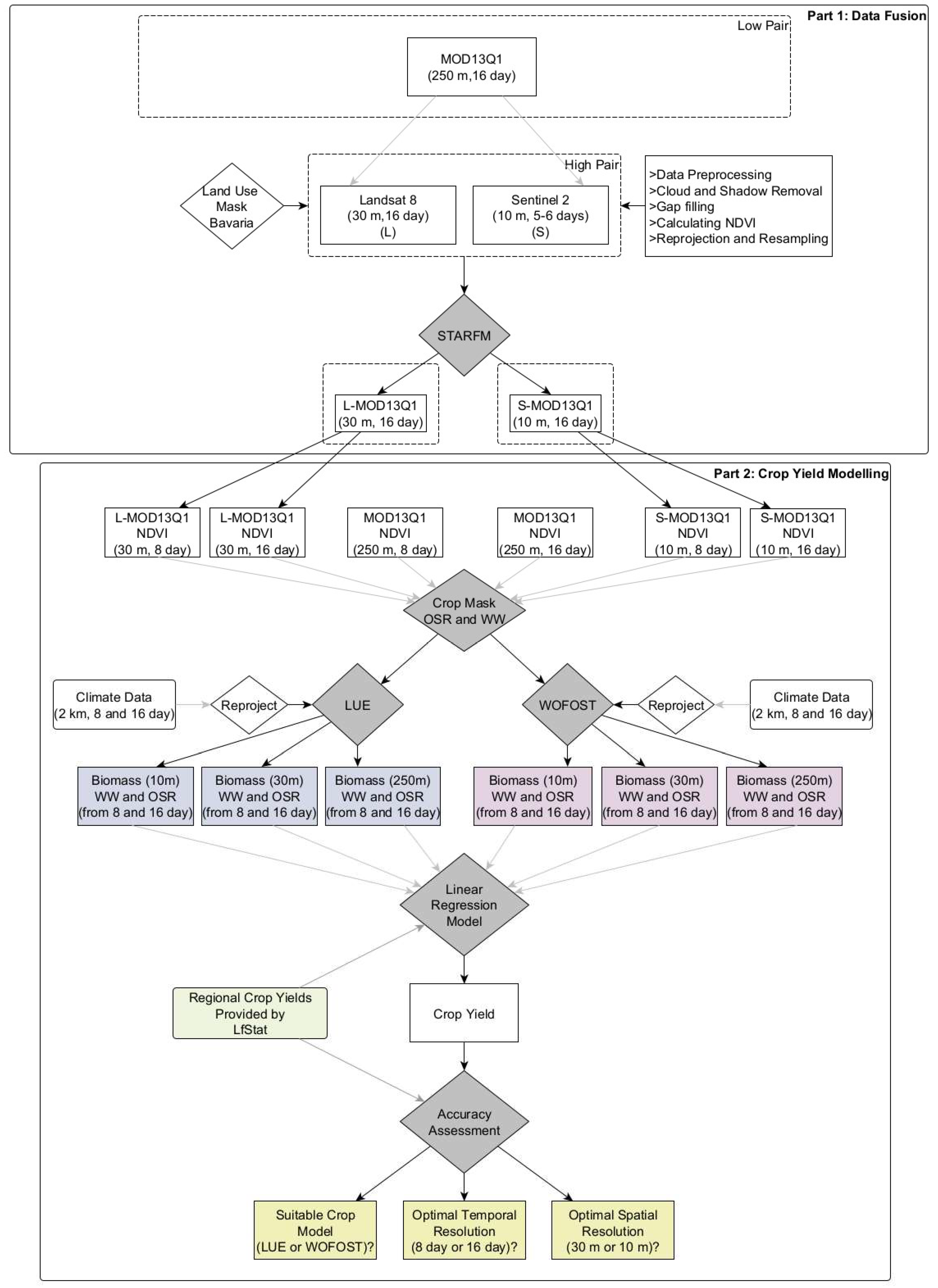
Figure 1. The conceptual framework of this study is divided into two parts: Part 1 states the data fusion for 2019 to investigate the synthetic NDVI time series product (this section was completed in our previous study [4]) and Part 2 estimates and validates the crop yield for Bavaria by inputting the fused L-MOD13Q1 time series and climate elements to a semi-empiric Light Use Efficiency (LUE) model. STARFM = Spatial and Temporal Adaptive Reflectance Fusion Model; NDVI = Normalised Difference Vegetation Index; L-MOD09GQ = Landsat-MOD09GQ; L-MOD09Q1 = Landsat-MOD09Q1; L-MCD43A4 = Landsat-MCD43A4; L-MOD13Q1 = Landsat-MOD13Q1; S-MOD09GQ = Sentinel-2-MOD09GQ; S-MOD09Q1 = Sentinel-2-MOD09Q1; S-MCD43A4 = Sentinel-2-MCD43A4; S-MOD13Q1 = Sentinel-2-MOD13Q1; LfStat = the Bayerisches Landesamt für Statistik (LfStat).
Remotesensing 15 01830 g001
Figure 2. An overview of the study region. The LC map of Bavaria is obtained by combining multiple inputs of Landcover maps, such as Amtliche Topographisch-Kartographisches Informationssystem, Integrated Administration Control System (provides the crop field information), and Corine LC, into one map. Agriculture (peach green) dominates mainly in the northwest and southeast of Bavaria, while forest and grassland classes (dark green and yellow, respectively) dominate in the northeast and south. The district map of Bavaria overlays the LC map. The enlargement (displayed with a dark red box on the top right map) shows the urban area of the town Volkach, including the oil seed rape (OSR) fields (dark orange) and the winter wheat (WW) fields (dark green). A brief description of the regions of Bavaria is shown in Figure A1.
Remotesensing 15 01830 g002
Figure 3. The cloud-free scenes are available for Landsat (in red box) and Sentinel-2 (in blue box) during the seasons of OSR and WW. Four cloud-free scenes were collected for the Landsat data and six were collected for the Sentinel-2 data. The maps show the NDVI values from −1 to 1 for Bavaria during 2019. The negative NDVI values indicate non-vegetated areas such as water bodies or barren land.
Remotesensing 15 01830 g003
Figure 4. Field-wise comparison of STARFM and real-time NDVI values of (a) MOD13Q1, (b) Landsat 8, (c) L-MOD13Q1, (d) Sentinel-2, and (e) S-MOD13Q1 on DOY 145 (25 May 2019) on WW fields. The image in (f) shows the spatial location of 10,000 random points in Bavaria used to draw line and bar plots in Figure 5 for comparing the mean NDVI values on a DOY basis for the real and synthetic NDVI products.
Remotesensing 15 01830 g004
Figure 5. The (a) line and (b) bar plots show the DOY-based and interquartile-range-based comparison of STARFM-generated NDVI values with their respective high-resolution input (Landsat (L) or Sentinel-2 (S)) and low-resolution input MOD13Q1, respectively. The comparison is based on the mean values extracted for 10,000 random points (whose spatial location is shown in Figure 4f) taken for the entire Bavaria.
Remotesensing 15 01830 g005
Figure 6. The scatter plots (al) compare the accuracies of LUE- and WOFOST-modelled yields (inputting the 8- and 16-day MOD13Q1, L-MOD13Q1 and S-MOD13Q1) with the referenced yield of WW. The green dots represent WW. Every plot contains a solid line to visualise the correlation of pixels between the referenced and modelled yield values.
Remotesensing 15 01830 g006
Figure 7. The scatter plots (al) compare the accuracies of LUE- and WOFOST-modelled yields (inputting the 8- and 16-day MOD13Q1, L-MOD13Q1, and S-MOD13Q1) with the referenced yield of OSR. The orange dots represent OSR. Every plot contains a solid line to visualise the correlation of pixels between the referenced and modelled yield values.
Remotesensing 15 01830 g007
Figure 8. The violin plots compare the crop yields of referenced (at 95% confidence interval) and modelled yields obtained from multi-source data (MOD13Q1, L-MOD13Q1, and S-MOD13Q1) at 8 and 16 days of temporal scales of (a,b) WW and (b,d) OSR using the (a,c) LUE and (b,d) WOFOST models in 2019. The green-coloured text represents WW and the orange-coloured text represents OSR. The text values represent the median yield values of every product.
Remotesensing 15 01830 g008
Figure 9. The box plots compare the accuracies (a,c) R2 and (b,d) RMSE of referenced (at 95% confidence interval) and modelled yields obtained from multi-source data: MOD13Q1, L-MOD13Q1, and S-MOD13Q1 at temporal scales of 8 and 16 days.
Remotesensing 15 01830 g009
Figure 10. Spatial distribution of referenced yields and predicted yields for WW using MOD13Q1 (8 and 16 days), L-MOD13Q1 (8 and 16 days), and S-MOD13Q1 (8 and 16 days) with LUE and WOFOST models for the state of Bavaria. The white colour represents no data available. A detailed map of the administrative regions of Bavaria is shown in Figure A1.
Remotesensing 15 01830 g010
Figure 11. The dot plots show the region-wise distribution of referenced yields and modelled yields obtained from multi-source data (MOD13Q1 (8 and 16 days), L-MOD13Q1 (8 and 16 days), and S-MOD13Q1 (8 and 16 days)) for WW using (a) LUE and (b) WOFOST in 2019. The regional referenced yields are displayed in red dots.
Remotesensing 15 01830 g011
Figure 12. Spatial distribution of referenced yields and predicted yields for OSR using MOD13Q1 (8 and 16 days), L-MOD13Q1 (8 and 16 days), and S-MOD13Q1 (8 and 16 days) with LUE and WOFOST models for the state of Bavaria. The white colour represents no data available. A detailed map of the administrative regions of Bavaria is shown in Figure A1.
Remotesensing 15 01830 g012
Figure 13. The dot plots show the region-wise distribution of referenced yields and modelled yields obtained from multi-source data (MOD13Q1 (8 and 16 days), L-MOD13Q1 (8 and 16 days), and S-MOD13Q1 (8 and 16 days)) for OSR using (a) LUE and (b) WOFOST in 2019. The regional referenced yields are displayed in red dots.
Remotesensing 15 01830 g013aRemotesensing 15 01830 g013b
Figure 14. The box plots show the comparison of accuracies (a,c) R2 values and (b,d) RMSE values obtained from the referenced yields (at 95% confidence interval), with LUE (a,b) and WOFOST (c,d) modelled yields including climate stress factors (dark blue and pink) and the modelled yields excluding the climate stress factors (sensitivity analysis) (light blue and pink).
Remotesensing 15 01830 g014aRemotesensing 15 01830 g014b
Figure 15. The dot plots show the comparison of accuracies for (a) R2, (b) RMSE, (c) RRMSE, and (d) ME values obtained from the referenced yields (at 95% confidence interval) for LUE (dark blue) and WOFOST (dark pink) models.
Remotesensing 15 01830 g015aRemotesensing 15 01830 g015b
Figure 16. The box plots compare the accuracies for (a) R2 and (b) RRMSE of referenced (at 95% confidence interval) and modelled yields obtained from multi-source data using LUE and WOFOST models in 2019.
Remotesensing 15 01830 g016
Figure 17. Visualisation of field level biomass of L-MOD13Q1 and S-MOD13Q1 with 8 days, 16 days, and the difference (16–18 days) obtained using the LUE model for (a) WW and (b) OSR.
Remotesensing 15 01830 g017
Table 1. A summary of the collected datasets for crop modelling of winter wheat (WW) and oil seed rape (OSR) in 2019. The satellite data used for crop yield modelling are synthetic L-MOD13Q1, S-MOD13Q1, and real Moderate Resolution Imaging Spectroradiometer (MODIS) MOD13Q1. The climate parameters are minimum temperature (°C) (Tmin), maximum temperature (°C) (Tmax), dewpoint temperature (°C) (Tdew), solar radiation (MJ m−2 day−1) (Rs), sunshine duration (hours) (N), evaporation (mm) (Ep), transpiration (mm) (Tp), runoff (mm) (Roff), and precipitation (mm) (P). InVeKos data provide the fields of WW and OSR for Bavaria in 2019; the Bayerisches Landesamt für Statistik (LfStat) data provide the crop yield information (dt/ha) of WW and OSR at the district level of Bavaria in 2019.
DataProduct NameResolution (Spatial-Temporal)References
Climate dataTmin, Tmax, Tdew, Rs, N, Ep, Tp, Roff, P2000 m, 8 and 16 dayshttps://www.uni-augsburg.de/de/fakultaet/fai/geo/ (accessed on 21 June 2021)
Satellite dataL-MOD13Q130 m, 8 and 16 days[4]
S-MOD13Q110 m, 8 and 16 days[4]
MODIS (MOD13Q1)250 m, 8 and 16 dayshttps://lpdaac.usgs.gov/ (accessed on 21 June 2021)
Vector dataInVeKos2019www.ec.europa.eu/info/index_en (accessed on 21 June 2021)
LfStat2019https://www.statistikdaten.bayern.de/genesis/online/ (accessed on 21 June 2021)
Table 2. Statistical analysis between the NDVI values obtained from raw Landsat (L) and Sentinel-2 (S) images with synthetic images (L- and S-MOD13Q1) on different days of the year (DOY). The analysis shows the R2 and mean RMSE obtained between the synthetic and reference NDVI in Bavaria for the land cover class of agriculture (which covers 31.67% of Bavaria) and for the overall classes (including agriculture, forest, urban, water, natural, semi-natural, and grassland) in 2019.
NDVI ProductLC ClassDOY
OSRWW
498197Mean
R2
Mean RMSE113145177Mean
R2
Mean RMSE
L-MOD13Q1Agriculture0.410.49-0.450.11-0.660.650.650.10
Overall0.430.50-0.470.11-0.610.620.620.11
S-MOD13Q1Agriculture0.490.740.850.690.100.760.500.600.620.12
Overall0.480.670.800.650.130.810.640.650.700.13
Table 3. A summary of equations used to calculate LAI from NDVI satellite products for WW and OSR. These equations are derived from the growth stage of a crop until the flowering stage. The LAI product is used as an input to the WOFOST model.
Crop TypeEquationR2References
WW L A I = 16.606 + 20.612 N D V I 0.70[61]
OSR L A I = 0.393 + 4.769 N D V I 0.81[62]
Disclaimer/Publisher’s Note: The statements, opinions and data contained in all publications are solely those of the individual author(s) and contributor(s) and not of MDPI and/or the editor(s). MDPI and/or the editor(s) disclaim responsibility for any injury to people or property resulting from any ideas, methods, instructions or products referred to in the content.