Article

Shadow Enhancement Using 2D Dynamic Stochastic Resonance for Hyperspectral Image Classification

1
College of Automation and Electronic Engineering, Qingdao University of Science and Technology, Qingdao 266061, China
2
College of Electromechanical Engineering, Qingdao University of Science and Technology, Qingdao 266061, China
3
College of Information Science and Engineering, Ocean University of China, Qingdao 266100, China
*
Author to whom correspondence should be addressed.
Remote Sens. 2023, 15(7), 1820; https://doi.org/10.3390/rs15071820
Submission received: 17 February 2023 / Revised: 21 March 2023 / Accepted: 27 March 2023 / Published: 29 March 2023

Abstract

:
With the development of remote sensing technology, classification has become a meaningful way to explore the rich information in hyperspectral images (HSIs). However, various environmental factors may cause noise and shadow areas in HSIs, resulting in weak signals and difficulties in fully utilizing information. In addition, classification methods based on deep learning have made considerable progress, but features extracted from most networks have much redundancy. Therefore, a method based on two-dimensional dynamic stochastic resonance (2D DSR) shadow enhancement and convolutional neural network (CNN) classification combined with an attention mechanism (AM) for HSIs is proposed in this paper. Firstly, to protect the spatial correlation of HSIs, an iterative equation of 2D DSR based on the pixel neighborhood relationship was derived, which made it possible to perform matrix SR in the spatial dimension of the image, instead of one-dimensional vector resonance. Secondly, by using the noise in the shadow area to generate resonance, 2D DSR can help increase the signals in the shadow regions by preserving the spatial characteristics, and enhanced HSIs can be obtained. Then, a 3DCNN embedded with two efficient channel attention (ECA) modules and one convolutional block attention module (CBAM) was designed to make the most of critical features that significantly affect the classification accuracy by giving different weights. Finally, the performance of the proposed method was evaluated on a real-world HSI, and comparative studies were carried out. The experimental results showed that the proposed approach has promising prospects in HSIs’ shadow enhancement and information mining.

Graphical Abstract

1. Introduction

Owing to remote sensing technology’s rapid growth, hyperspectral images (HSIs) containing rich information in the spatial and spectral dimensions [1] have extensive use in agricultural production [2], urban planning [3], environmental monitoring [4], and so on. By assigning category labels to each image pixel according to the sample characteristics, classification has become one of the effective means to extract information from HSIs [5].
Classical classification methods, including support vector machine (SVM) [6], k-nearest neighbor (K-NN) [7], maximum likelihood estimation (MLE) [8], dimension-reduction-based methods [9], linear discriminant analysis (LDA) [10], independent component analysis (ICA) [11], principal component analysis (PCA) [12], etc., have been used for HSI classification with good properties. However, they either need to reduce the dimensions of the data or can only obtain shallow features. In recent years, deep learning with a strong performance in extracting nonlinear features has been successfully applied to hyperspectral data processing [13]. The principle of deep learning classification is to extract features from basic to deep without pre-designing features. As an effective feature extraction method in image processing, convolutions can help obtain a feature map of an image after the convolutional operations. By arranging and combining low-level features at a higher level from the input layer to the output layer of the network, the features of an image are continuously extracted and abstracted, and classification and recognition can be achieved based on these features ultimately [14]. Typical networks such as the deep belief network (DBN) [15] and stacked auto-encoder (SAE) [16] can obtain deep features by layered training on the premise that the input should be converted to a one-dimensional vector. Besides, there are studies and achievements based on the graph neural network (GNN) designed for and targeted at irregular data, i.e., social networks and molecular networks [17,18].
Frameworks evolved from convolutional neural networks (CNNs), such as generative adversarial networks (GANs) [19] and Res-Net [20], can extract features with the consideration of both the spatial and the spectral information [21]. However, many feature maps within a layer show much pattern similarity, so that these features could be redundant, which means that, if one model has extracted information from one feature map, it will only need to extract the difference from its similar ones [22]. Meanwhile, on account of the single structure of these frameworks, all features are considered of equal importance, and some critical features influencing the classification effect significantly have not been made full use of. Therefore, the attention mechanism has emerged and is introduced to the convolutional neural network to evaluate the importance of the extracted features to ensure that the essential features are taken seriously enough in the classification [23,24].
However, due to the influence of cloud cover, light, and other environmental factors, some HSIs contain shadow areas, in which signals are weakened and information extraction, including classification, is difficult [25]. The HSIs spatial–spectral information enhancement can bring positive effects to HSIs’ classification [26,27]. The conventional approaches in the spatial domain and the transform domain for image enhancement [28,29], such as Retinex [30], histogram correction [31], the low pass filter (LPF) [32], the autoregressive moving average (ARMA) filter [33], and so on, mainly focus on removing noise, which would inevitably result in the loss of some signals and may destroy the correlation of the data [34]. There are methods based on neural networks for image enhancement [35] with time-consuming calculations and insufficient samples. Currently, the exploration of rich information in the shadow of hyperspectral images is still a difficult point in existing research. Using resonance generated by noise to improve the signal, one-dimensional dynamic stochastic resonance (DSR) has been introduced to enhance the signal with noise [25]. However, a two-dimensional spatial image must be converted to a one-dimensional vector before being processed by 1D DSR, which will inevitably destroy the spatial correlation of the image.
Therefore, an iterative equation of 2D DSR was derived in this paper, which can protect the spatial correlation of HSIs by performing matrix SR in the spatial dimension of the image instead of one-dimensional vector resonance. Furthermore, to fully utilize critical features that affect the classification result substantially, a 3DCNN embedded with two efficient channel attention (ECA) modules and one convolutional block attention module (CBAM) is proposed. By distributing the corresponding weights to the feature maps of the input, the attention mechanism can help the model make estimates more accurate without more consumption of the storage and computation of the model. The performance of the proposed shadow enhancement and classification approach was verified on a real-world HSI.
In this paper, on the one hand, the derivation of 2D DSR can not only develop the signal enhancement ability, but also protect the spatial correlation of image signals, laying the foundation for further information extraction. On the other hand, with two efficient channel attention modules and one convolutional block attention module, an improved 3DCNN was designed to fully utilize the key features and increase the classification performance.
The remaining content of this paper is organized as follows: Section 2 introduces the basic theories of the proposed technique, including the principles of the nonlinear bistable DSR system, the basic construction of the CNN, the derivation of 2D DSR based on the pixel neighborhood relationship, and the structure of the CNN with attention modules; Section 3 introduces the experimental details and results; Section 4 presents the comparison and discussion; Section 5 gives the conclusion.

2. Materials and Methods

2.1. Dynamic Stochastic Resonance

In image processing, noise affects the quality of the image and usually needs to be removed to increase the signal-to-noise ratio (SNR) of the image. However, the valuable signals in the image, especially the correlation between the signals, might inevitably be destroyed by the noise reduction when the noise spectrum is close to the signal spectrum. In some specific nonlinear systems, with stochastic resonance occurring, internal or external noise can help to enhance weak signals because some noise energy can be transferred into signal energy, and then, the SNR of the system output can be increased [36,37]. DSR is a spatial domain analysis method that correlates the bistable system parameters of the double-well potential with the intensity value of the noisy image.
On the basis of Langevin’s equation of motion, the 1D nonlinear expression of the overdamped dynamic system can be [38]
d h ( t ) d t = d H ( h ) d h + I ( t ) + μ ( t )
where I ( t ) is the periodic input signal, μ ( t ) is the intensity distribution of the noise, and t and h ( t ) are the time and spatial location of a particle moving in a bistable potential well. H ( h ) is the potential function affected by the displacement:
H ( h ) = 1 2 a h 2 + 1 4 b h 4
where a and b are system parameters. Figure 1 plots the situation a = b = 2.
Substitute Equation (2) for H ( h ) in Equation (1), then
d h ( t ) d t = a h ( t ) b h 3 ( t ) + I ( t ) + μ ( t )
where x ± = ± a b are the two stable points in Equation (3) and Δ H = a 2 4 b is a barrier of the system. If the periodic driving force, i.e., the periodic input signal I ( t ) , is absent, the system remains stable. If a periodic force is imposed on the bistable system, the system’s stability will be damaged and periodic changes will occur in the potential well. By cooperating with the periodic driving force, noise can provide energy for the particles to transform in two stable states. In other words, noise can help the signal obtain higher energy in the stochastic resonance system.

2.2. Convolutional Neural Network

With a deep structure including convolutional calculation, the CNN has been extensively applied to text, voice, image, video processing, and pattern recognition [39]. Based on the matrix-weight-sharing structure, representation learning ability, and shift invariance, the CNN has become a suitable model for processing HSI data [40]. The main structure of the CNN, including the input, convolutional, pooling, fully connected (FC), and output layers, is illustrated in Figure 2.
The input layer of the CNN can process multidimensional data. In the convolutional layers, convolutional kernels can extract features from the input data, and the activation function can make it easier to express complicated features. The convolution operation can be expressed as [41]
C H n l = A ( m = 1 M n = 1 N C H m l 1 s n l + r n l )
where C H n l is the n-th characteristic matrix of the l-th layer, A(·) indicates the activation function, M and N represent the number of neurons in the last and the current layer, respectively, and s n l and r n l are the weight matrix and offset of the corresponding convolution kernel.
After feature extraction, the output feature maps are transferred to the pooling layer to select features and filter information. The pooling layer can decrease the dimension of the feature map by downsampling, which can significantly cut down the number of neurons and the computational difficulty of the network.
By using the existing higher-order features, the fully connected layer can be combined with the nonlinear extracted features to gain the output. The feature map can be expanded into vectors in a fully connected layer by connecting each neuron with all the neurons in the previous layer.
The logic or softmax activation function is generally used to output classification labels for image classification. The commonly used softmax function can be expressed as
g ( O u t F C ) = s o f t m a x ( w g O u t F C + O f f s e t )
where w and O f f s e t are the vectors of the weight and offset and O u t F C is the output of the FC layer.
Currently, the CNN has different convolution kernels according to the dimension of the input data, including 1-dimensional (1D), 2D, and 3D, which have the same element calculation process and adopt backpropagation to modify the parameters.

2.3. Two-Dimensional DSR Shadow Enhancement for Hyperspectral Image Classification by CNN Embedded with Multiple Attention Mechanisms

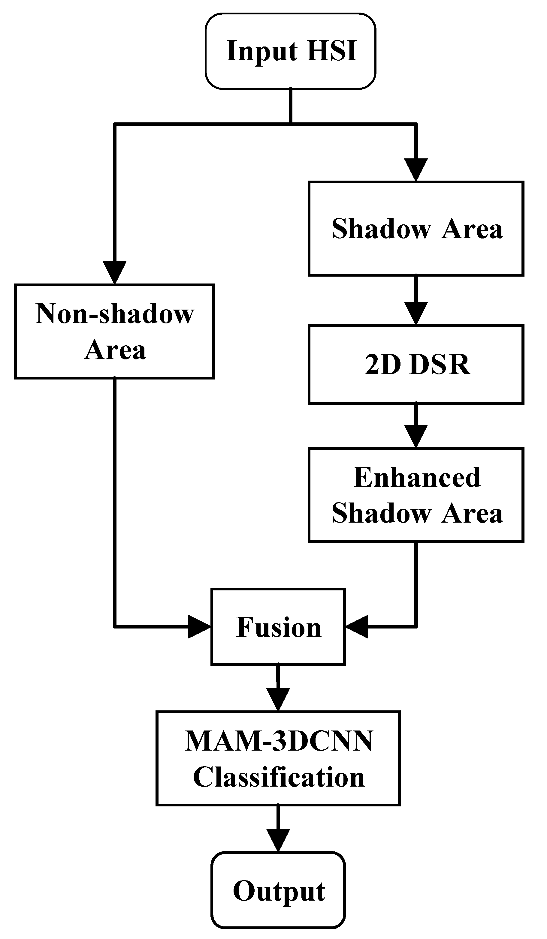
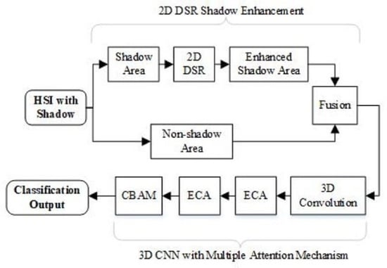
Because of light, cloud cover, and other environmental factors, there are shadow regions in some HSIs where signals are weak and information can hardly be analyzed. Meanwhile, all features extracted by the classification methods based on deep learning are generally considered equally important, so a few key features that seriously affect the classification result cannot be effectively made use of. Therefore, an iterative equation of 2D DSR was derived to enhance the signal in shadow areas, and a 3DCNN embedded with multiple attention mechanisms (MAM-3DCNN) is proposed for HSI classification in this paper. The proposed approach’s main procedure is shown in Figure 3.

2.3.1. Two-Dimensional Dynamic Stochastic Resonance

Classical stochastic resonance theory mainly deals with 1-dimensional vectors, so 2-dimensional and multidimensional data must be converted to 1 dimension before resonance processing. To preserve the spatial correlation of HSIs, an iterative equation of 2-dimensional DSR carrying out stochastic matrix resonance in the spatial dimension was derived.
For the shadow areas in HSIs, there are both a weak signal I ^ ( x , y ) and noise μ ^ ( x , y ) with x and y being the spatial position of the pixel. Denoting f ^ = I ^ ( x , y ) + μ ^ ( x , y ) and according to the 1D DSR in Equation (1), a 2D nonlinear expression of the bistable stochastic resonance system can be
h 2 ( x , y ) x y = θ ( h x + h y ) + a ^ h ( x , y ) b ^ h 3 ( x , y ) + f ^ ( x , y )
where h ( x , y ) is the system output and θ ( > 0 ) is the damping term of the system.
If the damping term h 2 ( x , y ) x y is large, the second-order term in Equation (6) can be ignored [42], and Equation (6) can be rewritten as
0 = ( h x + h y ) + a ^ θ h ( x , y ) b ^ θ h 3 ( x , y ) + f ^ ( x , y ) θ
By replacing a ^ θ , b ^ θ , and f ^ ( x , y ) θ with a, b, and f ( x , y ) , respectively, Equation (6) can be simplified as the following overdamped partial differential equation:
h ( x , y ) x + h ( x , y ) y = a h ( x , y ) b h 3 ( x , y ) + f ( x , y )
Based on the characteristic line theory [43], Equation (8) can be equivalent to two ordinary differential equations:
d x 1 = d h a h b h 3 + f d y 1 = d h a h b h 3 + f
where the characteristic line here is d x 1 = 1 , i.e., y = x + C with C being a constant. Therefore, in any small neighborhood, the interpretation of Equation (9) is symmetric about the diagonal direction [43], and solving the equations can be equivalent to independently solving the following equations:
d h d x = a h b h 3 + f ( x ) d h d y = a h b h 3 + f ( y )
The equivalent difference form of Equation (10) can be expressed as [44]
h i , j , k = t x [ a h i , j 1 , k b h i , j 1 , k 3 + f i , j 1 , k ] + h i , j 1 , k h i , j , k = t y [ a h i 1 , j , k b h i 1 , j , k 3 + f i 1 , j , k ] + h i 1 , j , k
where i, j are the abscissa and ordinate positions in the spatial dimension of the input shadow data f, k represents the k-th band of the HSI, i.e., f i , j 1 , k is the pixel at the (i, j 1 ) spatial position on the k-th band, t x and t y represent the sampling interval in the direction of abscissa and ordinate, respectively, and h i , j , k is the output of the system at (i, j) on the k-th band.
Since Equation (11) means nonlinear filtering of the input into horizontal and vertical directions at the same time, it can be extended to a four-way parallel difference form with the iterative update:
h i , j , k ( n + 1 ) = t x [ a h i , j 1 , k ( n ) b h i , j 1 , k 3 ( n ) + f i , j 1 , k ] + h i , j 1 , k ( n ) h i , j 1 , k ( n + 1 ) = t x [ a h i , j , k ( n ) b h i , j , k 3 ( n ) + f i , j , k ] + h i , j , k ( n ) h i 1 , j , k ( n + 1 ) = t y [ a h i , j , k ( n ) b h i , j , k 3 ( n ) + f i , j , k ] + h i , j 1 , k ( n ) h i , j , k ( n + 1 ) = t y [ a h i 1 , j , k ( n ) b h i 1 , j , k 3 ( n ) + f i 1 , j , k ] + h i 1 , j , k ( n )
where n indicates the number of iterations. The iterative process of Equation (12) on the k-th band of the HSI by 2D DSR is shown in Figure 4. Each pixel’s output combines spatial information in the upper, lower, left, and right directions, so that the correlation between the spatial pixels can be maintained.

2.3.2. Three-Dimensional Convolutional Neural Network with Multiple Attention Mechanisms

To exert the potential value of critical features that significantly impact the classification results, multiple attention modules were embedded into a 3DCNN. On the one hand, as a local cross-channel interaction strategy without dimension reduction, ECA can significantly improve network performance and avoid the adverse effect of compression and dimensionality reduction on the dependence between learning channels [45]. On the other hand, as a lightweight general module, a CBAM can be integrated into any CNN by adding a channel attention (CA) mechanism and a spatial attention (SA) mechanism to emphasize the channel and spatial characteristics [46]. In addition, HSIs have spectral data in hundreds of dimensions, resulting in complex channel states in the network, so double ECAs were inserted in the CNN and proven to be more effective in learning channel attention than one ECA through experiments. The main structure of the proposed MAM-3DCNN for HSI classification is illustrated in Figure 5.
Based on the aggregated features obtained by the global average pooling, ECA can generate channel weights by a fast 1D convolution, and the specific structure is illustrated in Figure 6.
The convolutional block attention module is composed of spatial attention and channel attention in series, as shown in Figure 7. In the CA of the CBAM shown in Figure 8, the global average pooling (GAP) and global maximum pooling (GMP) are firstly used to aggregate the spatial information of the input feature map, then the number of channels is compressed to C/r, with r being the compression ratio to reduce the parameter overhead, and the channel feature vectors can be obtained by elementwise summation finally. As a supplement to the channel attention, in the SA, the average pooling and maximum pooling are performed and an effective feature descriptor is generated by connecting the results, then a standard convolutional layer connection and convolution are combined to generate a 2D spatial attention map.

2.3.3. The Procedure of the Proposed MAM-3DCNN

In actual HSIs’ processing, the HSIs with shadows are three-dimensional data with a length (L), width (W), and height (H), and this can be represented as M H × W × L , where L represents the number of bands in the spectral dimension. The 2D data in each band can be defined as χ = [ X 1 , X 2 , , X L ] , and the pixel at (p,q) in the b-th band is X p , q b . Therefore, the specific steps can be carried out in detail:
Step 1: Firstly, a shadow mask needs to be set to extract the shadow area χ s d = [ X s d 1 , X s d 2 , , X s d L ] in the HSI.
Step 2: For the extracted data, 2D DSR in Equation (12) can be applied to each band of the data X s d b to enhance each pixel X s d ( p , q ) b by making use of the spatial information in the neighborhood, and then, the enhanced shadow data χ s d e d can be obtained.
Step 3: By fusing the enhanced shadow data with non-shadow data, the 2D DSR-enhanced HSI χ e n h a n c e d can be acquired.
Step 4: To reduce the impact of unrelated information and computing costs, the most-important 10 components are extracted by principal component analysis (PCA) before classification.
Step 5: Finally, the dimensionality reduced data are divided according to the window size as the constructed classification network’s input to obtain the final result.

3. Experiment

To assess the performance of the proposed approach, a real-world HSI dataset was used and the experiments were carried out in the Ubuntu 16.04 operating system on an NIVIDIA GTX2080Ti with 11GB memory. The programs and models were built on Keras.

3.1. Dataset

The real-world Hyperspectral Digital Imagery Collection Experiment (HYDICE) data with a shadow area were adopted in this paper. With a 0.75 m spatial resolution and a 10nm spectral resolution, it consists of 316 rows, 216 columns, and 148 spectral bands from 435 to 2326 nm. Figure 9 lists the original HYDICE image and the ground truth. The labels and the number of samples are presented in Table 1. In the classification experiments, the HYDICE data were randomly divided into training and test subsets without overlap, with the test subset accounting for 80%.
To compare the classification results quantitatively, as commonly used evaluation indices for HSIs, the overall accuracy (OA), average accuracy (AA), and Kappa coefficients were introduced to the experiments [47]. The OA can be defined as
O A = u U R u , v G × 100 %
where U indicates the number of labels, R with the size of U × U is the confusion matrix, R u , v represents samples belonging to label u, but misclassified into label v, and G is the number of the tested samples.
Correspondingly, the A A and K a p p a coefficients can be expressed as below:
A A = 1 U u U R u , u v U R u , v × 100 %
K a p p a = G u U R u , v u U v U ( R u , v × R v , u ) G 2 u U v U ( R u , v × R v , u ) × 100 %
Besides, the classification accuracy of each category was calculated by the recall value, which indicates the correctly predicted positive samples and is calculated as:
R e c a l l = R u , u v U R u , v

3.2. Parameter Setting

3.2.1. Setup of 2D DSR Parameters

The setting of the parameters in DSR directly affects the depth of the potential well, the barrier and the vibration state of the system, etc. However, there is no straightforward algorithm to determine the parameter values of a specific given resonance system, and in practice, the values are determined numerically by fitting various applications. The number of parameters to be set in 2D DSR increases from 2 in 1D DSR to 5, which are a, b, t x , t y , and n in Equation (12).
Since the purpose of DSR enhancement in this paper was to improve the classification accuracy of ground targets in shadow areas, the OA was used to measure the rationality of the parameter settings. With a, b, t x , and t y from 0 to 5 and n from 1 to 10, the enhanced image can be acquired by fusing the shadow area processed by 2D DSR with the non-shadow area and then classified by the 3DCNN. According to the above principle, the appropriate parameter for the HYDICE image in Figure 9 can be set as t x = t y = a = b = 0.01 and n = 5. The OA values under different n are shown in Figure 10.

3.2.2. Parameter Setting of MAM-3DCNN

In the experiments, to obtain a stable network performance, the internal parameters of the MAM-3DCNN in Figure 5, Figure 6, Figure 7 and Figure 8 were set as shown in Table 2, and the configuration of the network operation is displayed in Table 3. Moreover, through network debugging, setting the parameters p in Figure 6 to 3 and r in Figure 8 to 1 was suitable for the HYDICE HSI. The OA, AA, and Kappa values under different parameter settings of r are shown in Figure 11.

3.3. Experimental Results

3.3.1. Shadow Enhancement by 2D DSR

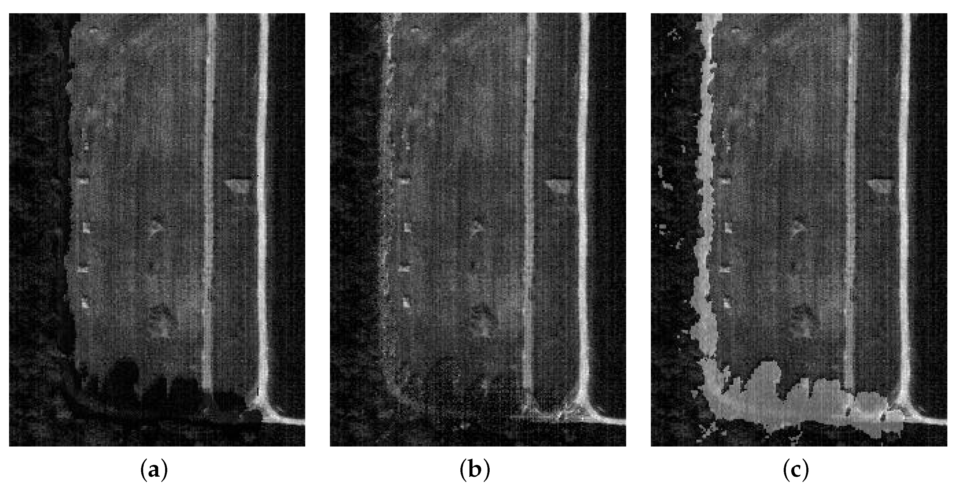
Theoretically, the expansion of DSR from 1D to 2D can maintain the spatial correlation of the HSI data, so the effect of shadow enhancement by 1D DSR [25] and 2D DSR was focused on in this paper. Firstly, the HYDICE data were normalized to meet the small parameter requirements of DSR. Secondly, a shadow mask constructed from the ground truth in Figure 8b was applied to acquire the shadow data in HYDICE. Then, each band of the extracted image can be processed by 2D DSR in Equation (12). Finally, the HSI with an enhanced shadow area could be attained by fusing the enhanced shadow area with the original image. The results of HYDICE enhanced by 1D and 2D DSR are shown in Figure 12, and the classification accuracy of 3DCNN is illustrated in Table 4.
Compared to the original HYDICE in Figure 12a, 1D DSR can help promote the information expression of the HSI and the ground objects were clearer than before visually. However, the image of the 2D-DSR-enhanced data in the first dimension had lighter brightness, which reduced the impact of the shadow to a greater extent. The effect can be verified as well in the information extraction experiment by the 3DCNN. As shown in Table 4, compared with the classification results of the original data and the 1D-DSR-enhanced data, the application of 2D DSR increased the OA by 0.812% and 0.3231%, the AA by 1.2116% and 1.1483%, and Kappa by 1.3432% and 0.6837%. The application of 1D DSR had a positive effect in improving the information expression, and the classification accuracy can be promoted. Whether in the evaluation of the OA, AA, or Kappa coefficient, the information extraction effect for 2D-DSR-enhanced data was better, which proved the superiority of 2D DSR in spatial information utilization and had great performance in HSI shadow enhancement.

3.3.2. Classification Results

To concentrate on the improvement of the classification methods based on the CNN, the 2D and 3DCNN combined with different attention mechanisms often used for the CNN, for instance the squeeze-and-excitation module (SE) [48], global attention block (GAB) [49], dual attention (DA) [50], double ECA (DECA), and CBAM, were compared, and the classification results of the considered methods are listed in Table 5 and Figure 13. Compared with the other methods, the OA and Kappa values achieved the best effect, increasing the OA value by 1.2441%, 1.2369%, 0.9498%, 0.319%, 0.2223%, 0.3358%, 0.4234%, 0.1952%, 0.1677%, 0.1364% and Kappa value by 2.1509%, 2.1274%, 1.1969%, 0.5421%, 0.3838%, 0.2307%, 0.5743%, 0.7304%, 0.4032%, 0.4009%, and 0.2139%, and the AA value of the proposed technique was 90.9980%, only next to that of the 3DCNN. By observing the recall of the compared methods, the proposed method had a better effect for most labels’ classification, especially for Target 1, Target 2, and Target 3, the recall values being 0.88%, 4.43%, and 2.86% higher than the 3DCNN.
According to the values of the evaluation indices in Table 5, it can be known that the classification accuracy of 2DCNN-based methods was not as good as that of 3DCNN-based methods. Similar inferences can be drawn from the classification results in Figure 13, especially for the “Road in shadow” pixels. In Figure 13a, some pixels belonging to “Road in shadow” were misclassified into “Tree in shadow” in orange color, because the 2DCNN can only use the spatial information of images, but not the spectral information of HSIs, which plays a vital role in identifying target categories. With the introduction of the attention mechanisms to the 2DCNN, more pixels of “Road in shadow” in Figure 13b,c were correctly classified than in Figure 13a. The 3DCNN can fully utilize the three-dimensional tensor properties of HSIs, which include both spatial and spectral information, so its classification performance Figure 13d is superior to the 2DCNN. Compared with the results in Figure 13 from (d) to (l), for pixels in the lower-right corner, the classification of the 3DCNN was still rough, which indicated the effectiveness of the attention modules. Moreover, due to the single channel attention concentration, the OA values of the GAB-3DCNN, SE-3DCNN, and ECA-3DCNN were lower than 97.50%, and the CBAM combining both channel and spatial attention can better help improve the classification than the former modules. In addition, hundreds of dimensions of spectral data in HSIs lead to complex channel states in the network, so double ECAs, as in Figure 13j, can be more effective at learning channel attention than one ECA, as in Figure 13i, especially when they are combined with the CBAM, as in Figure 13l; the effect is significant.

4. Discussion

4.1. Analysis of 2D DSR Effect on Shadow Enhancement

As shown in Figure 14, the spectral curves of road and grass in the shadow area before and after 2D DSR enhancement are plotted, respectively. It can be observed that the enhancement effect was obvious; specifically, the spectral curve of enhanced grass showed a similar trend for non-shadow grass in Figure 14b.
Compared with the original HYDICE image in Figure 12a, 2D DSR can significantly enhance the shadow area, especially in the 1∼40 bands with Figure 14 observed at the same time, while 1D DSR had a relatively weak enhancement effect. Table 4 shows that the application of DSR can effectively promote the classification performance by improving the ability of image feature expression. The proposed 2D DSR improved the OA, AA, and Kappa values by 0.8120%, 1.2116%, and 1.3432%, respectively, which were 0.3231%, 1.1483%, and 0.6837% higher than the classification accuracy of 1D DSR, indicating the positive impact of 2D DSR on information mining.

4.2. The Classification Performance Discussion of Considered Measures

As shown in Table 5, benefiting from large samples, all considered methods had a good performance on grass classification. Compared to the 2DCNN and 3DCNN, the attention mechanism had a particular effect of improving the network’s performance. Because the 3DCNN can make full use of the 3D data characteristics of HSIs, the classification effect of the method based on the 3DCNN was better than that based on the 2DCNN. Although the GAB-3DCNN, 3DCNN, and ECA-3DCNN performed better on road, road in shadow, and grass in shadow than the other methods, with an overview of all labels, the classification effect of the MAM-3DCNN was prominent. In addition, the MAM module improved the OA and Kappa values of the 3DCNN by 0.3190% and 0.5421%. According to the classification accuracy of the different methods shown in Figure 15, the proposed method performed better than the other considered methods under the evaluation of the OA, AA, and Kappa, among which the AA values were the lowest. Only the AA values of the 3DCNN and MAM-3DCNN were close, but the difference between the AA value of the MAM-3DCNN and the best AA value was only 0.0493%.
Furthermore, according to the classification accuracy shown in Table 5, ECA had a certain effect on extracting the channel attention by increasing the influence of the feature map with a large effect, with the OA and Kappa values improving by 0.1238% and 0.1389%. With the channel and spatial attention combined, the CBAM also had a good function in improving the OA and Kappa values of the 3DCNN by 0.1809% and 0.3114%. The MAM-3DCNN combines the advantages of both the ECA and CBAM attention mechanisms, which can enlarge the impact of key feature maps to a greater extent through dual-channel attention and spatial attention. The pixels of most categories can be classified by the MAM-3DCNN more accurately than the other considered methods, especially for the small samples Targets 1, 2, and 3, whose OA values improved by 0.88%, 4.43%, and 2.86%, respectively.
It can be observed in Figure 13 that most of the considered methods were not good at the classification of road in shadow in the lower left, but the error classification rate of the MAM-3DCNN was lower than the other methods. From Table 5 and Figure 13, the 3DCNN embedded ECA, specially the MAM-3DCNN, can effectively classify labels with few samples, such as grass in shadow, Target 1, and Target 2. Except for the MAM-3DCNN, other methods based on the 3DCNN misclassified some of the leftmost pixels belonging to the tree as grass, as shown in Figure 13e–i. Therefore, the proposed MAM-3DCNN method can help to improve the classification accuracy for enhanced HSIs.
The comparison with the methods based on the GNN [51] and GAN [21] is shown in Table 6. Owing to the function of 2D DSR shadow enhancement, the OA values of the 3D-GAN, MARP-GNN, and MAM-3DCNN improved by 0.8%, 0.94%, and 0.84%. It can be seen that the MAM-3DCNN performed better than the methods in Table 6 because the GNN is designed for irregular data processing and the GAN takes advantage of overcoming the difficulty of insufficient samples. In this paper, the HYDICE data were compatible with the multi-attention combined CNN classification.
Owing to the function of 2D DSR shadow enhancement, the results showed that the OA was improved by 0.8%, 0.94%, and 0.84% under the classification of the 3D-GAN, MARP-GNN, and MAM-3DCNN, respectively, which indicated that the more spatial information utilized by the 2D DSR proposed in this paper had a certain effect on the HSI information improvement and the classification accuracy can be promoted. Compared to the results of the methods based on the GAN and GNN, the MAM-3DCNN had better performance as well. The design of the GNN makes it better at irregular data processing, and the GAN has more advantage by overcoming the difficulty of insufficient samples. In this paper, the adopted data had better compatibility with the multi-attention combined CNN feature extraction.
For the 2DCNN, spectral information from HSIs is not considered, which is crucial for target classification, although attention mechanisms can improve its classification accuracy to some extent. Due to the ability of using both the spectral and spectral dimensional characteristics of the HSI data, the 3DCNN is suitable for processing HSIs. The incorporation of the attention mechanism, especially the embedding of double ECAs and CBAM, further improved the classification performance of the 3DCNN.

5. Conclusions

Due to complex environmental factors, there are shadow areas in some HSIs, which negatively affect the HSIs’ classification. Meanwhile, features extracted from most classification networks have much redundancy. Therefore, a shadow enhancement method based on 2D DSR and a classification model combining a CNN with multiple attention mechanisms for HSIs were proposed in this paper. Firstly, to maintain the spatial correlation of HSIs, an iterative equation of 2D DSR was derived. Next, the weak signal in the shadow area can be increased by 2D DSR, and enhanced HSIs can be obtained. Then, a 3DCNN embedded with two ECA modules and one CBAM was designed to utilize the key features significantly affecting the classification accuracy. Finally, a real-world HSI was used to estimate the performance of the proposed technique. The numerical results showed that 2D DSR outperformed 1D DSR in shadow enhancement of HSIs and the MAM-3DCNN had more competitive classification ability than other considered methods. By applying 2D DSR, the signals and the image quality in the shadow area can be improved. In addition, the HSI classification performance was upgraded by introducing multiple channel and spatial attention modules to the 3DCNN. Therefore, the proposed technique has potential prospects in the shadow information exploration of HSIs.
Although 2D DSR is convenient for processing the image matrix, the 3D tensor characteristic of HSIs was not taken into account. Therefore, these results encourage us to further expand DSR to 3D to protect the 3D data features of HSIs.

Author Contributions

Conceptualization, X.L.; data curation, Q.L. and M.F.; formal analysis, X.L.; funding acquisition, X.L. and M.F.; investigation, Q.L., X.L. and M.F.; methodology, X.L. and Q.L.; project administration, X.L. and M.F.; resources, X.L. and Q.L.; software, Q.L. and X.L.; supervision, X.L. and M.F.; validation, X.L., Q.L. and M.F.; visualization, Q.L. and X.L.; writing—original draft, Q.L. and X.L.; writing—review and editing, Q.L., X.L. and M.F. All authors have read and agreed to the published version of the manuscript.

Funding

This research was funded by the National Natural Science Foundation of China (Grant No. 61971244) and the Shandong Provincial Natural Science Foundation (Grant No. ZR2020MF011).

Data Availability Statement

Not applicable.

Acknowledgments

The authors would like to thank the Editors and Reviewers for their valuable comments.

Conflicts of Interest

The authors declare no conflict of interest.

References

  1. Ahmad, M.; Shabbir, S.; Roy, S.K.; Hong, D.; Wu, X.; Yao, J.; Khan, A.M.; Mazzara, M.; Distefano, S.; Chanussot, J. Hyperspectral Image Classification-Traditional to Deep Models: A Survey for Future Prospects. IEEE J. Sel. Top. Appl. Earth Obs. Remote Sens. 2022, 15, 968–999. [Google Scholar] [CrossRef]
  2. Wang, C.; Liu, B.; Liu, L.; Zhu, Y.; Hou, J.; Liu, P.; Li, X. A review of deep learning used in the hyperspectral image analysis for agriculture. Artif. Intell Rev. 2021, 54, 5205–5253. [Google Scholar] [CrossRef]
  3. Yuan, J.; Wang, S.; Wu, C.; Xu, Y. Fine-Grained Classification of Urban Functional Zones and Landscape Pattern Analysis Using Hyperspectral Satellite Imagery: A Case Study of Wuhan. Artif. Intell. Rev. 2022, 15, 3972–3991. [Google Scholar] [CrossRef]
  4. Zhu, C.; Ding, J.; Zhang, Z.; Wang, J.; Wang, Z.; Chen, X.; Wang, J. SPAD monitoring of saline vegetation based on Gaussian mixture model and UAV hyperspectral image feature classification. Comput. Electron. Agric. 2022, 200, 107236. [Google Scholar] [CrossRef]
  5. Zeng, J.; Hu, W.; Huang, F. Analysis of Hyperspectral Image Classification Technology and Application Based on Convolutional Neural Networks. In Proceedings of the IEEE International Conference on Computer Science, Fuzhou, China, 24–26 September 2021; pp. 409–414. [Google Scholar] [CrossRef]
  6. Kaul, A.; Raina, S. Support vector machine versus convolutional neural network for hyperspectral image classification: A systematic review. Concurr Comput. 2022, 34, e6945. [Google Scholar] [CrossRef]
  7. Bo, C.; Lu, H.; Wang, D. Spectral-spatial K-Nearest Neighbor approach for hyperspectral image classification. Multimed. Tools Appl. 2018, 77, 10419–10436. [Google Scholar] [CrossRef]
  8. Peng, J.; Li, L.; Tang, Y. Maximum Likelihood Estimation-Based Joint Sparse Representation for the Classification of Hyperspectral Remote Sensing Images. IEEE Trans. Neural Netw. Learn Syst. 2019, 30, 1790–1802. [Google Scholar] [CrossRef]
  9. Li, H.; Cui, J.; Zhang, X.; Han, Y.; Cao, L. Dimensionality Reduction and Classification of Hyperspectral Remote Sensing Image Feature Extraction. Remote Sens. 2022, 14, 4579. [Google Scholar] [CrossRef]
  10. Shambulinga, M.; Sadashivappa, G. Supervised hyperspectral image classification using svm and linear discriminant analysis. Int. J. Comput. Appl. 2020, 11, 403–409. [Google Scholar] [CrossRef]
  11. Jayaprakash, C.; Damodaran, B.B.; Viswanathan, S.; Soman, K.P. Randomized independent component analysis and linear discriminant analysis dimensionality reduction methods for hyperspectral image classification. J. Appl. Remote Sens. 2020, 14, 1. [Google Scholar] [CrossRef]
  12. Uddin, M.P.; Mamun, M.A.; Hossain, M.A. PCA-based Feature Reduction for Hyperspectral Remote Sensing Image Classification. IETE Tech. Rev. 2021, 38, 377–396. [Google Scholar] [CrossRef]
  13. Li, S.; Song, W.; Fang, L.; Chen, Y.; Pedram, G.; Benediktsson, J.A. Deep learning for hyperspectral image classification: An overview. IEEE Trans. Geosci. Remote Sens. 2019, 57, 6690–6709. [Google Scholar] [CrossRef] [Green Version]
  14. Zhao, Y.; Zhang, X.; Feng, W.; Xu, J. Deep Learning Classification by ResNet-18 Based on the Real Spectral Dataset from Multispectral Remote Sensing Images. Remote Sens. 2022, 14, 4883. [Google Scholar] [CrossRef]
  15. Li, C.; Wang, Y.; Zhang, X.; Gao, H.; Yang, Y.; Wang, J. Deep belief network for spectral-spatial classification of hyperspectral remote sensor data. Sensors 2019, 19, 204. [Google Scholar] [CrossRef] [PubMed] [Green Version]
  16. Zhou, P.; Han, J.; Cheng, G.; Zhang, B. Learning Compact and Discriminative Stacked Auto-encoder for Hyperspectral Image Classification. IEEE Trans. Geosci. Remote Sens. 2019, 57, 4823–4833. [Google Scholar] [CrossRef]
  17. Ding, Y.; Zhang, Z.; Zhao, X.; Cai, W.; He, F.; Cai, Y.; Cai, W. Deep hybrid: Multi-graph neural network collaboration for hyperspectral image classification. Def. Technol. 2022, in press. [CrossRef]
  18. Ding, Y.; Zhang, Z.; Zhao, X.; Hong, D.; Cai, W.; Yu, C.; Yang, N.; Cai, W. Multi-feature fusion: Graph neural network and CNN combining for hyperspectral image classification. Neurocomputing 2022, 501, 246–257. [Google Scholar] [CrossRef]
  19. Ding, F.; Guo, B.; Jia, X.; Chi, H.; Xu, W. Improving GAN-based feature extraction for hyperspectral images classification. J. Electron. Imaging 2021, 30, 063011. [Google Scholar] [CrossRef]
  20. Abdulsamad, T.; Chen, F.; Xue, Y.; Wang, Y.; Yang, L.; Zeng, D. Hyperspectral image classification based on spectral and spatial information using ResNet with channel attention. Opt. Quantum Electron. 2021, 53, 1–20. [Google Scholar] [CrossRef]
  21. Zhang, F.; Bai, J.; Zhang, J.; Xiao, Z.; Pei, C. An Optimized Training Method for GAN-Based Hyperspectral Image Classification. IEEE Geosci. Remote S. 2021, 18, 1791–1795. [Google Scholar] [CrossRef]
  22. Zhang, Q.; Jiang, Z.; Lu, Q.; Han, J.N.; Zeng, Z.; Gao, S.H.; Men, A. Split to Be Slim: An Overlooked Redundancy in Vanilla Convolution. arXiv 2020, arXiv:2006.12085. [Google Scholar] [CrossRef]
  23. Huang, Y.; Zhang, L.; Huang, C.; Qi, W.; Song, R. Parallel Spectral–Spatial Attention Network with Feature Redistribution Loss for Hyperspectral Change Detection. Remote Sens. 2023, 15, 246. [Google Scholar] [CrossRef]
  24. Shi, C.; Sun, J.; Wang, T.; Wang, L. Hyperspectral Image Classification Based on a 3D Octave Convolution and 3D Multiscale Spatial Attention Network. Remote Sens. 2023, 15, 257. [Google Scholar] [CrossRef]
  25. Liu, X.; Wang, H.; Meng, Y.; Fu, M. Classification of Hyperspectral Image by CNN Based on Shadow Area Enhancement through Dynamic Stochastic Resonance. IEEE Access. 2019, 7, 134862–134870. [Google Scholar] [CrossRef]
  26. Zhou, L.; Ma, X.; Wang, X.; Hao, S.; Ye, Y.; Zhao, K. Shallow-to-Deep Spatial-Spectral Feature Enhancement for Hyperspectral Image Classification. Remote Sens. 2023, 15, 261. [Google Scholar] [CrossRef]
  27. Zhou, J.; Zeng, S.; Xiao, Z.; Zhou, J.; Li, H.; Kang, Z. An Enhanced Spectral Fusion 3DCNN Model for Hyperspectral Image Classification. Remote Sens. 2022, 14, 5334. [Google Scholar] [CrossRef]
  28. Qi, Y.; Yang, Z.; Sun, W.; Lou, M.; Lian, J.; Zhao, W.; Deng, X.; Ma, Y. A Comprehensive Overview of Image Enhancement Techniques. Arch. Comput. Method Eng. 2022, 29, 583–607. [Google Scholar] [CrossRef]
  29. Yu, T.; Zhu, M. Image Enhancement Algorithm Based on Image Spatial Domain Segmentation. Comput. Inform. 2021, 40, 1398–1421. [Google Scholar] [CrossRef]
  30. Wang, Y.; Wang, Y.; Han, Q.; Wang, Y.; Li, Y.; Han, Q.; Li, Y.; Li, Y. Low Illumination Image Enhancement based on Improved Retinex Algorithm. J. Comput. 2022, 33, 127–137. [Google Scholar] [CrossRef]
  31. Deng, W.; Liu, L.; Chen, H.; Bai, X. Low Infrared image contrast enhancement using adaptive histogram correction framework. Optik 2022, 271, 170114. [Google Scholar] [CrossRef]
  32. Shao, P.; Yang, L.; Li, X. Finite impulse response low-pass digital filter based on particle swarm optimization for image denoising. Wirel Commun. Mob. Comput. 2021, 20, 41–47. [Google Scholar] [CrossRef]
  33. Ding, Y.; Zhao, X.; Zhang, Z.; Cai, W.; Yang, N.; Zhan, Y. Semi-Supervised Locality Preserving Dense Graph Neural Network with ARMA Filters and Context-Aware Learning for Hyperspectral Image Classification. IEEE Trans. Geosci. Remote Sens. 2022, 60, 1–12. [Google Scholar] [CrossRef]
  34. Li, C.; Li, Z.; Liu, X.; Li, S. The Influence of Image Degradation on Hyperspectral Image Classification. Remote Sens. 2022, 14, 5199. [Google Scholar] [CrossRef]
  35. Sobbahi, R.A.; Tekli, J. Comparing deep learning models for low-light natural scene image enhancement and their impact on object detection and classification: Overview, empirical evaluation, and challenges. Signal Process Image Commun. 2022, 109, 116848. [Google Scholar] [CrossRef]
  36. Li, H.; Zheng, H.; Han, C.; Wang, H.; Miao, M. Onboard Spectral and Spatial Cloud Detection for Hyperspectral Remote Sensing Images. Remote Sens. 2018, 10, 152. [Google Scholar] [CrossRef] [Green Version]
  37. Yang, Y.; Tao, W.; Huang, J.; Xu, B. Over exposed image information recovery via stochastic resonance. Chin. Phys. B 2012, 21, 305–311. [Google Scholar] [CrossRef]
  38. Kumar, A.; Jha, R.K.; Nishchal, N.K. Dynamic stochastic resonance and image fusion based model for quality enhancement of dark and hazy images. J. Electron. Imaging 2021, 30, 063008. [Google Scholar] [CrossRef]
  39. Hu, M.; Mao, J.; Li, J.; Wang, Q.; Zhang, Y. A novel lidar signal denoising method based on convolutional autoencoding deep learning neural network. Atmosphere 2021, 12, 1403. [Google Scholar] [CrossRef]
  40. Zhu, Q.; Zu, X. Fully Convolutional Neural Network Structure and Its Loss Function for Image Classification. IEEE Access. 2022, 10, 35541–35549. [Google Scholar] [CrossRef]
  41. Dai, D. An Introduction of CNN: Models and Training on Neural Network Models. In Proceedings of the 2021 International Conference on Big Data, Artificial Intelligence and Risk Management (ICBAR), Shanghai, China, 5–7 November 2021; pp. 135–138. [Google Scholar] [CrossRef]
  42. Risken, H. The Fokker-Planck Equation: Method of Solutions and Applications, 2nd ed.; Springer Series in Synergetics; Springer: Berlin, Germany, 1989. [Google Scholar]
  43. Courant, R.; Hilbert, D. Methods of Mathematical of Physics; Interscience Publ. Inc.: New York, NY, USA, 1953; Voluem 1, p. 173. [Google Scholar]
  44. Lapidus, L.; Pinder, G.F. Numerical Solution of Partial Differential Equations in Science and Engineering; John Wiley and Sons, Inc.: New York, NY, USA, 1982. [Google Scholar]
  45. Yang, Q.; Ku, T.; Hu, K. Efficient attention pyramid network for semantic segmentation. IEEE Access 2021, 9, 18867–18875. [Google Scholar] [CrossRef]
  46. Ju, A.; Wang, Z. Convolutional block attention module based on visual mechanism for robot image edge detection. EAI Endorsed Trans. Scalable Inf. Syst. 2018, 9, 172214. [Google Scholar] [CrossRef]
  47. Liu, X.; Wang, H.; Liu, J.; Sun, S.; Fu, M. HSI Classification Based on Multimodal CNN and Shadow Enhance by DSR Spatial-Spectral Fusion. Can. J. Remote Sens. 2021, 47, 773–789. [Google Scholar] [CrossRef]
  48. Hu, J.; Shen, L.; Albanie, S.; Sun, G.; Wu, E. Squeeze-and-Excitation Networks. IEEE Trans. Pattern Anal. Mach. Intell. 2019, 42, 1. [Google Scholar]
  49. Chen, Y.; Xing, M. A global attention-based convolutional neural network for process prediction. In Proceedings of the 2022 41st Chinese Control Conference (CCC), Hefei, China, 25–27 July 2022. [Google Scholar] [CrossRef]
  50. Li, X.; Xie, M.; Zhang, Y.; Ding, G.; Tong, W. Dual attention convolutional network for action recognition. IET Image Process. 2020, 14, 1059–1065. [Google Scholar] [CrossRef]
  51. Zhang, Z.; Ding, Y.; Zhao, X.; Siye, L.; Yang, N.; Cai, Y.; Zhan, Y. Multireceptive field: An adaptive path aggregation graph neural framework for hyperspectral image classification. Expert Syst. Appl. 2023, 217, 119508. [Google Scholar] [CrossRef]
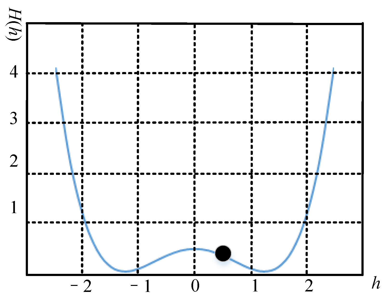
Figure 1. Situation of the system with a = b = 2.
Remotesensing 15 01820 g001
Figure 2. The main structure of the CNN. Conv1 and Conv2 represent Convolutional Layers 1 and 2. Pooling1 and Pooling2 stand for Pooling Layers 1 and 2.
Remotesensing 15 01820 g002
Figure 3. The main procedure of the proposed approach.
Remotesensing 15 01820 g003
Figure 4. The iterative process of 2D DSR on the k-th band of the HSI. A 2 × 2 window is used to slide the sampling. The dashed lines of different types represent relevant pixels involved in updating the enhancement value of a pixel through Equation (11). The ①,…, ④ correspond to the relationship between the pixels in the first to fourth sub-formulas in Equation (12). I × J represents the size of the data in each band of the HSI.
Remotesensing 15 01820 g004
Figure 5. The main structure of the proposed MAM-3DCNN. The size of the convolutional kernel is 3 × 3 × 3 , and the 8 3DConv means 3D convolution with 8 convolutional kernels. GAP is the global average pooling. ⊗ denotes the positionwise dot product. The 256 FC1 is the 1st fully connected layer with 256 neurons.
Remotesensing 15 01820 g005
Figure 6. The specific structure of ECA. The input feature maps’ height and width are represented by H and W, and C is the number of channels. p represents the required adjacent channels to obtain the cross-channel interaction information of each channel and can be adaptively determined via a mapping of C. Sigmoid is the activation function.
Remotesensing 15 01820 g006
Figure 7. The basic structure of the CBAM. The channel attention module assesses the importance of each channel and gives the input channels the corresponding weights, and the spatial attention offers different attention to pixels in each channel according to the significance.
Remotesensing 15 01820 g007
Figure 8. The detailed structure of the CA and SA in the CBAM. The H × W × C represents the data with the H height, W width, and C channels. r is the compression ratio. ⊕ denotes elementwise summation. Mean and Max represent the average pooling and maximum pooling. Concat means feature fusion.
Remotesensing 15 01820 g008
Figure 9. The original HYDICE and ground truth. (a) HYDICE. (b) Ground truth.
Remotesensing 15 01820 g009
Figure 10. OA values under different n. The best result is obtained when n = 5.
Remotesensing 15 01820 g010
Figure 11. Comparison of classification accuracy under different rs. The best result of the OA, AA, and Kappa can be obtained when r = 1.
Remotesensing 15 01820 g011
Figure 12. The 1 S T band of HYDICE enhanced by 1D and 2D DSR. (a) Original HYDICE; (b) 1D DSR; (c) 2D DSR.
Remotesensing 15 01820 g012
Figure 13. Classification results: (a) 2DCNN; (b) GAB-2DCNN; (c) MAM-2DCNN; (d) 3DCNN; (e) GAB-3DCNN; (f) CBAM-3DCNN; (g) SE-3DCNN; (h) DA-3DCNN; (i) ECA-3DCNN; (j) DECA-3DCNN; (k) ECA-CBAM-3DCNN; (l) MAM-3DCNN.
Remotesensing 15 01820 g013
Figure 14. Comparison of spectral curves. Solid, dashed, and dotted lines represent the spectral curves of road and grass not in the shadow area, in the shadow areas, and after enhancement, respectively. (a) Spectral curves of road. (b) Spectral curves of grass.
Remotesensing 15 01820 g014
Figure 15. The values of the OA, AA, and Kappa of the considered methods.
Remotesensing 15 01820 g015
Table 1. Information of the ground truth. The labels, sample number, and represented colors for each category in the ground truth are displayed.
NumberColorSampleLabel
1 33,184Grass
2 10,850Tree
3 3376Road
4 1686Road in shadow
5 323Grass in shadow
6 537Target 1
7 514Target 2
8 4135Target 3
Table 2. Internal parameter setting of the MAM-3DCNN.
LayerKernelKernel SizeActivationDropout
3DConv83 × 3 × 3Relu-
MAMECA11DConv1p = 3Sigmoid-
ECA21DConv1p = 3Sigmoid-
CBAMFC3/FC5 (3DConv)81 × 1 × 1Relu-
FC4/FC6 (3DConv)81 × 1 × 1--
3DConv13 × 3 × 3Sigmoid-
FC1256-Relu0.6
FC2128-Relu0.5
Table 3. Configuration of the network operation.
NameSetting
Window size11
Test ratio0.8
Learning rate0.001
OptimizerAdam
Epoch100
Loss functionCategorical cross-entropy
Table 4. Classification accuracy of different data by the 3DCNN.
DataOriginalEnhanced by
1D DSR
Enhanced by
2D DSR
OA96.538897.027797.3508
AA89.835789.899091.0473
Kappa94.093694.753195.4368
Table 5. Classification accuracy of the considered methods. The 2DCNN and 3DCNN with different attention modules are included.
Method2D
CNN
GAB-
2DCNN
MAM-
2DCNN
3D
CNN
GAB-
3DCNN
CBAM-
3DCNN
SE-
3DCNN
DA-
3DCNN
ECA-
3DCNN
DECA-
3DCNN
ECA-
CBAM-
3DCNN
MAM-
3DCNN
Grass0.99000.99000.99000.99000.99000.99000.99000.99000.99000.99000.99000.9900
Tree0.97250.97000.97500.98200.98400.98600.98200.98000.98600.98600.98550.9869
Road0.95500.96000.96450.97000.97400.97200.97400.96800.96800.96900.96950.9700
Road in
shadow
0.79250.82600.83200.88200.84200.86200.85600.85600.85200.85200.84300.8538
Grass in
shadow
0.89750.89600.90200.94400.92200.91800.92400.91600.92800.91200.91200.9138
Target 10.84250.87600.89460.89200.87600.89400.88400.87200.88400.88560.88600.9008
Target 20.66250.69200.72200.71800.62600.70600.63400.60200.64200.66500.71300.7623
Target 30.87750.85200.86000.90600.93200.93200.92000.91800.92600.92000.92300.9346
OA (%)96.425796.432996.720097.350897.447597.531797.334097.246497.474697.502197.533497.6698
AA (%)87.295888.305388.575091.047389.349090.766689.626688.789289.870789.880690.102390.9980
Kappa (%)93.828093.851594.482095.436895.595195.748295.404695.248595.575795.578095.765095.9789
Table 6. Classification of the original and 2D-DSR-enhanced HYDICE by methods based on the GNN and GAN.
Evaluation3D-GANMARP-GNNMAM-3DCNN
HYDICE2D DSRHYDICE2D DSRHYDICE2D DSR
OA (%)96.2297.0296.4497.3896.8397.67
AA (%)87.3390.1388.5090.3589.6191.00
Kappa (%)93.4994.3694.5595.1394.5295.98
Disclaimer/Publisher’s Note: The statements, opinions and data contained in all publications are solely those of the individual author(s) and contributor(s) and not of MDPI and/or the editor(s). MDPI and/or the editor(s) disclaim responsibility for any injury to people or property resulting from any ideas, methods, instructions or products referred to in the content.