Can the Perception Data of Autonomous Vehicles Be Used to Replace Mobile Mapping Surveys?—A Case Study Surveying Roadside City Trees

Abstract

The continuous flow of autonomous vehicle-based data could revolutionize current map updating procedures and allow completely new types of mapping applications. Therefore, in this article, we demonstrate the feasibility of using perception data of autonomous vehicles to replace traditionally conducted mobile mapping surveys with a case study focusing on updating a register of roadside city trees. In our experiment, we drove along a 1.3-km-long road in Helsinki to collect laser scanner data using our autonomous car platform ARVO, which is based on a Ford Mondeo hybrid passenger vehicle equipped with a Velodyne VLS-128 Alpha Prime scanner and other high-grade sensors for autonomous perception. For comparison, laser scanner data from the same region were also collected with a specially-planned high-grade mobile mapping laser scanning system. Based on our results, the diameter at breast height, one of the key parameters of city tree registers, could be estimated with a lower root-mean-square error from the perception data of the autonomous car than from the specially-planned mobile laser scanning survey, provided that time-based filtering was included in the post-processing of the autonomous perception data to mitigate distortions in the obtained point cloud. Therefore, appropriately performed post-processing of the autonomous perception data can be regarded as a viable option for keeping maps updated in road environments. However, point cloud-processing algorithms may need to be adapted for the post-processing of autonomous perception data due to the differences in the sensors and their arrangements compared to designated mobile mapping systems. We also emphasize that time-based filtering may be required in the post-processing of autonomous perception data due to point cloud distortions around objects seen at multiple times. This highlights the importance of saving the time stamp for each data point in the autonomous perception data or saving the temporal order of the data points.

1. Introduction

Since 2010, more than EUR 300 billion have been invested in automation, connectivity, electrification, and smart mobility [1]. About two-thirds of this total investment has gone to autonomous vehicle technology and smart mobility. Autonomous vehicle technology is expected to be one of the most significant reforms that will affect society within the coming decades and it may change our way of living and working.

Autonomous vehicles have a large number of onboard sensors for monitoring the dynamic environment around the vehicle. The applied sensors can be categorized into two groups: ranging sensors and image-based sensors. Ranging sensors, such as sonar, radar, and LiDAR are active sensors measuring the surrounding scene in 3D [2]. The advantages of LiDAR include its high-ranging accuracy, high pulse repetition rate (PRF), and small beam divergence. These advantages enable the detection of small objects in the 3D space. However, the cost of LiDAR is high. Micro- and millimeter wave radars provide range, distances, and speed measurements. Since they have wider beams, the detection of objects is more difficult. Passive vision-based sensors collect photogrammetric data, enabling the detection of moving objects, traffic lights, and signs. Typical positioning techniques of an autonomous car include the use of global navigation satellite system (GNSS) data, inertial measurement units (IMUs), road paintings, other signals, wheel angles, and dead reckoning. Autonomous cars also use high-definition (HD) maps and simultaneous localization and mapping (SLAM) for GNSS-free positioning.

Similar sensors are also applied in mobile mapping systems, such as in Google’s Street View car. Mobile mapping is typically regarded as the process of collecting geospatial data from a mobile vehicle. However, there are multiple differences in the sensors and their arrangements between autonomous vehicles and mobile mapping vehicles. Firstly, the sensors of an autonomous vehicle typically provide a full 360° field of view around the vehicle with a focus on forward-looking sensors that enable perceiving objects 200–300 m ahead of the vehicle. Thus, objects may be visible for a long period of time in the perception data. On the other hand, designated mobile mapping systems traditionally have scanners viewing approximately the direction perpendicular to the driving direction and, therefore, the mapped objects are visible for a short period of time. The use of robotic systems for mobile mapping has also increased in recent years [3,4]. As the second difference, the laser scanners onboard autonomous systems typically have wide beam sizes due to the need to have full coverage of the view. On the contrary, the preferred beam size of surveying-grade laser scanners in mobile mapping systems is typically as small as possible.

As for the third difference, autonomous vehicles process perception data in real time with the aim to derive vehicle positions and driveable areas ahead of the vehicles while also detecting and classifying other objects in the surroundings. An autonomous car may make a high-definition map or even update it, but it does not measure object geometries accurately in real time. Loop-closure techniques are used to correct drifts in the data [5]. In contrast, the traditional process for mobile mapping systems includes turning raw sensory data into 3D georeferenced data, known as the 3D product [6]. The outcome of the mobile mapping system is a 3D map of the surroundings, including a description of the geometry of the objects. This traditional processing is done in a post-processing mode to obtain maximal accuracy. Since objects are visible for a short period of time, the algorithms for point cloud processing seldom utilize the time information of the data points in the 3D point cloud. However, there are notable exceptions, including, e.g., the use of robotic systems for mapping forest environments [7,8] or the use of strip adjustments for data processing [9].

When even a small number of autonomous vehicles with the abovementioned high-quality sensors exist, very large amounts of data will be collected from road environments on a continuous basis. Currently, there are, however, only a few papers that consider the emerging possibility of using the perception data for applications beyond autonomous driving, i.e., for autonomous big data analytics and applications that may have the potential for replacing traditionally used mobile mapping systems. If these big data can be exploited outside each car’s own real-time processing, this will open up totally new opportunities for the 3D monitoring and modeling of the urban, traffic, and road environments. For example, current procedures in topographic mapping are based on data specifically acquired for the purpose, and updating the map has not been properly solved due to the high costs. The continuous flow of autonomous vehicle-based data could change current procedures by providing interesting new ways for updating the map databases. In addition, such data would enable completely new types of near-real-time mapping applications, although appropriate post-processing would still be necessary. As the data generated by autonomous driving are massive (e.g., 2 TB/h), it would be impossible to transfer all of the data in real time to local computing centers. Therefore, we envision this to open up a new endeavor where the dynamic 3D mapping data can be ordered from a specified region (programmable mapping) and, thus, the collected data need to be transferred only upon request.

During the last 10 years, the possibility of utilizing perception data from autonomous vehicles for surveying applications has been briefly mentioned at a high level only in a few papers and public presentations related to developing national geospatial infrastructure, such as those in [10,11,12,13,14]. However, a more detailed review of such papers is provided in Section 2. To the best of our knowledge, the existing literature lacks any evidence of using autonomous perception data for surveying and mapping purposes in a post-processing mode that enables accurate measurements of roadside object geometries. We assume that data analysis methods may need to be developed individually for each case and system.

Therefore, in this article, we study the potential of autonomous perception data to replace mobile mapping surveys in precise road environment mapping applications when sophisticated post-processing methods are applied to the perception data. As a case study, we have selected the use of autonomous perception data to update the tree register of a city. Specifically, we examine the accuracy of estimating the stem curve and diameter at breast height (DBH) of urban trees from such data, as these attributes carry crucial information about the size of the trees. City trees are quite commonly managed using tree registers and mobile mapping is one feasible solution for creating and updating the registers [15,16,17]. For example, the city of Helsinki in Finland maintains a register of about 40,000 urban trees, including about 20,000 along-street trees. City tree registers are used, e.g., for deciding on maintenance operations, such as watering and pruning, so that trees are not in the way of cars, buses, trams, or electric air cables. The use of register data reduces maintenance costs. Updating a tree register manually is costly, and, therefore, automation is needed.

In summary, the original contributions of this paper are:

• We show that the perception data of an autonomous car can be used to replace designated mobile mapping surveys when the geometry of roadside objects, such as trees, is to be measured.
• As a case study, we measure the stem attributes of roadside trees for a city tree register using perception data of an autonomous car system.
• We compare the obtained accuracy against a conventional mobile laser scanning survey for the same trees.
• We discuss the data processing logic needed in general when post-processing perception data of autonomous cars for mapping and surveying applications.

This article is structured as follows: First, we review the existing literature on secondary usages of autonomous perception data in Section 2. In Section 3, we present the urban test area, the research platform for autonomous driving (known as ARVO), and introduce a mobile laser scanning system (ROAMER) that was utilized in this work to collect a reference laser scanning dataset from the same test area. The ROAMER system was developed for high-precision mobile mapping applications; thus, a comparison between the results obtained using the ARVO and ROAMER systems allows us to evaluate the strengths and weaknesses of autonomous perception data for acquiring roadside environmental data. The remainder of Section 3 presents the methods used for data processing culminating in a description of the algorithms used for stem curve estimation. Section 4 and Section 5 present and discuss the results while also considering potential surveying applications of autonomous perception data together with general requirements for the data processing logic. Finally, the conclusions are drawn in Section 6.

2. Short Review on Using Perception Data of Autonomous Vehicles for Surveying

This short review concentrates on the secondary usage of autonomous perception data that constitutes an example of big data. One can define big data in many ways [18]. According to Laney et al. (2001) [19], big data consist of three elements: volume (referring to the amount of data), velocity (referring to the need for capturing and analyzing data in time), and variety (referring to various data types). Mayer-Schönberger and Cukier (2013) stated that much of the value of big data is associated with secondary uses [20]. Importantly, this paper is about extracting more value from autonomous perception data with the secondary usage of data for road-environment mapping and applications.

A short summary of autonomous driving can be found in [21,22,23,24,25,26,27,28,29,30,31,32,33,34,35,36,37,38,39]. As mentioned in Section 1, the key real-time processes of autonomous cars include the positioning of the car, calculation of the driveable area, and detection and classification of road environment objects. Many open-access datasets related to autonomous driving exist, such as Kitti [40], the 3D Dataset [41], nuscenes [42], the Waymo open dataset [43], apolloscapes [44], and A2d2 [45]. Masello et al. (2022) performed a systematic review of a substantial number of vehicle datasets from all automation levels [46]. In the review, 68 self-driving datasets were found and analyzed for the self-driving task. To the best of our knowledge, such datasets have not been used to demonstrate the secondary use of autonomous perception data for surveying purposes using post-processing and time-based filtering. An obvious reason for this is the lack of field reference data. In the following, we briefly summarize the state-of-the-art in three different categories related to mapping with autonomous car data: (1) high-definition maps, (2) autonomous perception data used to assist autonomous driving, and (3) autonomous perception data used to assist surveying.

High-definition maps—a large number of articles focus on high-definition maps, i.e., high-definition (HD) maps, which aim to help with the positioning of an autonomous car (see, e.g., [13,28,31,47]). Automatic updating of HD maps is also a hot research topic. The HD maps are not, however, optimized for the derivation of the geometry of roadside objects, although they can provide a rough estimate of the geometry.

Autonomous perception data used to assist autonomous driving—Some papers have studied the potential of using big data to assist with autonomous driving. These technologies mainly focus on real-time processes. Seif and Hu (2016) proposed, without a detailed analysis, that big data analytics based on data acquired from robotic cars could enable new services for road users and governmental institutions [10]. According to them, the benefits would include optimizing traffic behavior, improving traffic control systems, and enhancing safety and security solutions. In the work by Xu et al. (2017) [14], autonomous big data applications, such as environmental perception, were mentioned but not analyzed. Al Najada and Mahgoub (2016) optimized the safe trajectory of an autonomous vehicle using data on real-life accidents and data from connected vehicles [11]. Daniel et al. (2017) [48] stated that telematics and real-time analysis will become future technologies of autonomous vehicles. In the work by Yoo et al. (2020) [49], a local dynamic map system was designed and implemented for the big data of connected cars. Local dynamic maps can be used to store dynamic data, such as weather, road quality, and traffic information for the use of autonomous cars. Wang et al. (2022) [50] provided insights based on existing studies on autonomous driving with the focus on automatic lane change maneuvers, obstacle detection, and trajectory prediction. Zhu et al. (2018) [51] reported several case studies on big data analytics in the context of intelligent transportation systems, including personal travel route plans, road traffic accident analyses, public transportation service plans, control and assets maintenance, rail transportation management, and road traffic flow prediction.

Autonomous perception data used to replace current surveying approaches—There are only a few papers focusing on the possibilities of utilizing autonomous perception data to replace current designated mobile mapping systems in mapping and surveying applications. Naturally, the use of SLAM in the autonomous car leads to a map of the surroundings, but such data may not be well-suited for mapping and surveying applications without further post-processing. In the work by Virtanen et al. (2017) [12], the potential of using autonomous perception data for mapping purposes was depicted. They envisioned a future where most cars will be equipped with a mobile mapping system, resulting in a continuous flow of road-side point cloud data. However, they did not demonstrate any case study using autonomous perception data. In the work by Hyyppä et al. (2018) [52], the use of autonomous perception data for updating roadside building vectors and monitoring roadside parking status was explained.

There are no detailed articles, to the knowledge of the authors, on the use of autonomous perception data for replacing current mapping and surveying approaches based on designated mobile mapping systems by employing post-processing of the autonomous perception data to measure object geometries. It is likely that the lack of access to a combined dataset containing both the autonomous perception data and the related field reference has hindered the progress in this field of research. Since the secondary use of autonomous perception data has tremendous potential in the upcoming decades, this is a new research area.

3. Material and Methods

In this section, we provide the details of the laser scanning measurements and algorithms that were used to assess the feasibility of autonomous perception data for the collection and analysis of roadside environmental data. First, we provide information on the test area and the manual field measurements of the roadside reference trees in Section 3.1. Subsequently, Section 3.2 discusses the acquisition of the autonomous perception data using the research platform for autonomous driving (ARVO) and the acquisition of a reference laser scanning dataset obtained with the help of the mobile mapping system ROAMER. In Section 3.3, we first present the data-processing steps required to convert the raw sensor data into a point cloud in a global coordinate frame in Section 3.3.1 and Section 3.3.2; afterward, we introduce the point cloud-processing methods in Section 3.3.3–Section 3.3.5, including the algorithms used to estimate the stem curve and the DBH of roadside trees. Finally, we present metrics for computing statistics of tree detection and stem-attribute estimation in Section 3.4.

3.1. Test Area

The study area was located on two streets, i.e., Pohjolankatu and Koskelantie in Käpylä, Helsinki, Finland (60°12′31″N, 24°57′1″E). On these streets, 139 roadside trees were selected as reference trees to assess the accuracy of urban tree measurements conducted by post-processing the collected autonomous perception data. The majority of reference trees were old linden trees. In total, the 139 reference trees corresponded to a road length of 1310 m. For each reference tree, manual field measurements of the stem diameters were conducted in March 2021 at five different heights to obtain accurate reference values for the stem curves, i.e., the stem diameters at various heights. As can be seen from Figure 1a, the manual stem diameter measurements were carried out by recording the circumference of the tree trunk with a tape measure at heights ranging from 1.0 to 3.0 m above the ground level. In

Table 1. Descriptive statistics of the roadside trees located in the test area based on the manual field measurements. The data in the table include the total number of reference trees, the total length of the road under study, mean of DBH, standard deviation of DBH, minimum DBH, maximum DBH, mean diameter of the stem curves, and the mean of the lowest and highest height, at which the stem diameter is manually measured.

Number of Trees	Road Length (m)	DBH				Stem Curve
		Mean (cm)	Std. (cm)	Minimum (cm)	Maximum (cm)	Mean (cm)	Minimum Height (m)	Maximum Height (m)
139	1310	49.3	12.5	23.0	83.8	49.2	1.0	2.9

, we summarize the descriptive statistics of the reference trees, including, e.g., the diameter at breast height (DBH).

Figure 1a–c illustrate three example reference trees. For some of the reference trees, the stem diameter varied significantly as a function of the height even over short distances due to deformations in the tree trunk. For some of the trees, the cross-sectional shapes of the tree trunks differed greatly from a circle, and the bark also tended to be thick and rough. All of these factors inevitably hampered the accuracy of stem diameter measurements conducted either via manual means or by using laser scanning technologies.

3.2. Data Acquisition

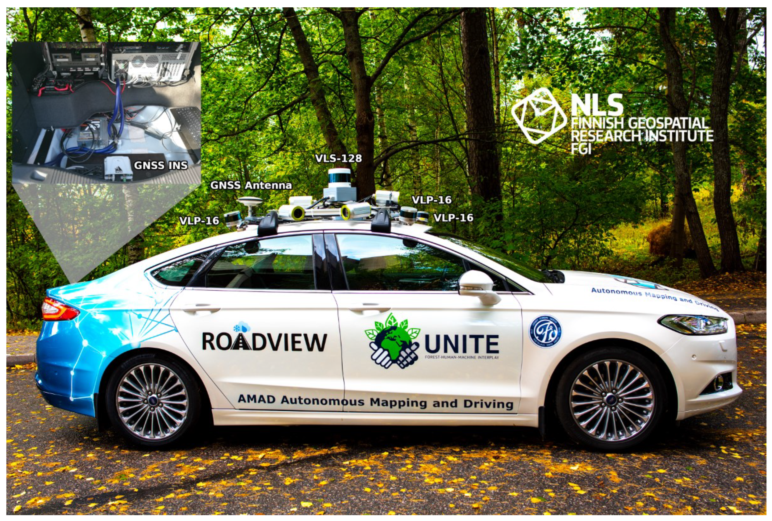
3.2.1. Autonomous Mapping and Driving Research Platform ARVO

The Autonomous Research Vehicle Observatory (ARVO), the autonomous mapping and driving research platform of the Finnish Geospatial Research Institute (FGI), was used for collecting the autonomous perception data used in this work. Previously, ARVO has been used as an autonomous car prototype in some of our past studies [47,53,54,55]. ARVO was built on a Ford Mondeo hybrid passenger vehicle equipped with the high-grade computational capacity and a perception sensor system designed for autonomous driving. The system currently comprises LiDARs, cameras, thermal cameras, and radar sensors. The sensor system contains five LiDAR sensors, four × Velodyne VLP-16 Puck LITE [56] LiDARs, one in each corner of the roof, and one × Velodyne VLS-128 Alpha Prime [57] on top of the roof. Figure 2 demonstrates the complete sensor system of ARVO. ARVO’s sensor system is complemented by NovAtel PwrPak7-E1 [58], a professional-grade global navigation satellite system (GNSS) inertial navigation system (INS), which is used for vehicle positioning and time synchronization of ARVO’s perception system.

In this work, only data from ARVO’s main LiDAR Velodyne VLS-128 and NovAtel GNSS INS were used. The Velodyne VLS-128 is a rotating multi-beam LiDAR with 128 lasers covering a vertical field of view of 40° ranging from −25° to 15° with respect to the horizontal direction. The data recording was handled with the Robot Operating System (ROS) [59] Kinetic Kame running on Ubuntu 16.04. Sensor drivers built on the ROS were used to interface the sensors and to record the raw data in the ROS bag format to ARVO’s onboard data storage. The data from the ARVO platform, used in this work, were recorded on 27 April 2020. An example of point cloud data recorded with the ARVO platform is shown in Figure 3.

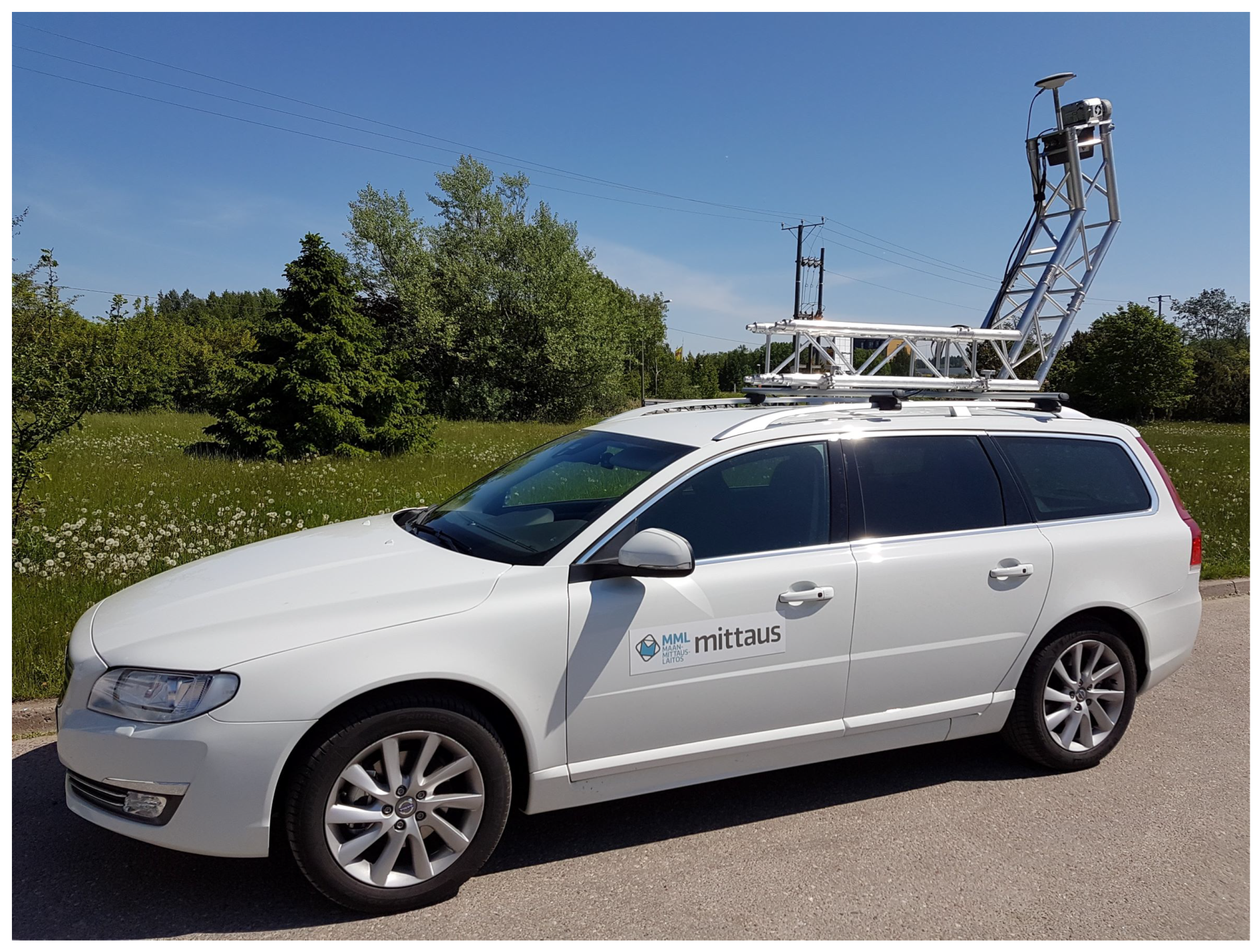
3.2.2. Mobile Mapping System ROAMER

FGI’s mobile laser scanning system ROAMER R3 was used to collect reference laser point cloud data. ROAMER R3 consists of survey grade sensors Riegl VUX-1HA laser scanner, integrated with NovAtel Flexpak6 GNSS receiver, Pinwheel 703GGG antenna, and NovAtel UIMU-LCI inertial measurement units. The trajectory output rate was 200 Hz. ROAMER R3 was installed on top of a car on a truss structure to achieve a better viewpoint for road-environment mapping, as illustrated in Figure 4. In the past, ROAMER was used in several dozens of studies; some of them are listed here: [61,62,63,64,65,66,67]. The laser scanning measurements with the ROAMER system were conducted at the test area on 24 November 2016.

3.3. Data Processing

In this section, we present the data processing steps that were utilized to detect roadside trees and estimate their stem curves and DBHs starting from the raw sensor data collected by the ARVO and ROAMER systems. In Section 3.3.1 and Section 3.3.2, we explain how the raw sensor data of the two systems were post-processed in order to obtain georeferenced 3D point clouds of the studied road environment. After converting the raw data into the point cloud format, we used the same algorithmic workflow to detect and measure the roadside trees for both systems. The stem-attribute retrieval algorithms used in this study are based on a slight modification of our earlier work [7,8]. We chose to use these algorithms since they enable the stem diameter and volume measurements of trees in a boreal forest with state-of-the-art-level root-mean-square errors of 5% and 10%, respectively, regardless of the point cloud distortions arising from time-dependent drifts.

As a brief summary, the stem-attribute retrieval process begins by finding the digital terrain model that is then subtracted from the z-coordinates of each point in the point cloud. Subsequently, arc-like structures with approximately circular shapes are searched in the point cloud since they potentially correspond to tree stems. Importantly, we use time-based filtering and divide the points into disjoint sets based on their time stamp before searching for the arc-like structures; as a result, the point cloud analysis is robust against point cloud distortions caused by moderate temporal drifts in the estimated laser scanner trajectory. The arc-like structures are detected using a series of steps including, e.g., DBSCAN clustering, RANSAC-based circle fitting, and a comparison against heuristic quality criteria to filter out unreliable arcs. After the arc detection step, the arc coordinates are clustered to detect individual trees and, subsequently, the stem diameter is estimated for each of the detected trees at various heights in a way that is robust against temporal drifts in the data. The end result is an estimate of the stem curve, i.e., diameter vs. height from the ground and the DBH for each detected tree. The data processing steps are visually summarized in the flow chart shown in Figure 5.

3.3.1. Post-Processing the Raw Sensor Data of the Autonomous Car System ARVO into a 3D Point Cloud

Data from the main LiDAR sensor Velodyne VLS-128 of ARVO are saved in the ROS bag format. Each ROS bag holds a collection of ROS messages, which are comprised of data packages with angle and distance information. The VLS-128 device driver contains a method for the computing point cloud in scanner-native coordinates. The point cloud computing method was modified to provide each point with time according to the device-firing time chart. For each point, the laser number, firing time, intensity, and location are saved. ARVO’s GNSS-INS sensor data are post-processed using NovAtel Inertial Explorer software [68]. The post-processed trajectory is used for georeferencing the VLS-128 point cloud in Matlab. The georeferencing is done in two steps: first, the VLS-128 point cloud is transformed to GNSS-INS coordinates using manually derived exterior orientation parameters, and second, the point cloud in GNSS-INS system coordinates is transformed using the time for each point and corresponding pose and location from the post-processed trajectory.

3.3.2. Post-Processing the Raw Sensor Data of the Mobile Mapping System ROAMER into a 3D Point Cloud

The GNSS-IMU data resulting from the ROAMER R3 system were post-processed using special software Waypoint Inertial Explorer (NovAtel, Galgary, AB, Canada), which computes differential GNSS corrections based on Trimnet network Virtual Reference Station (VRS) base station data and by using precise ephemeris and satellite clock data in a multi-pass process. Tightly coupled processing was applied to generate the initial trajectory. Riegl RiProcess software (version 1.8.8) was applied for boresight alignment calibration and LiDAR point cloud calculations based on the trajectory.

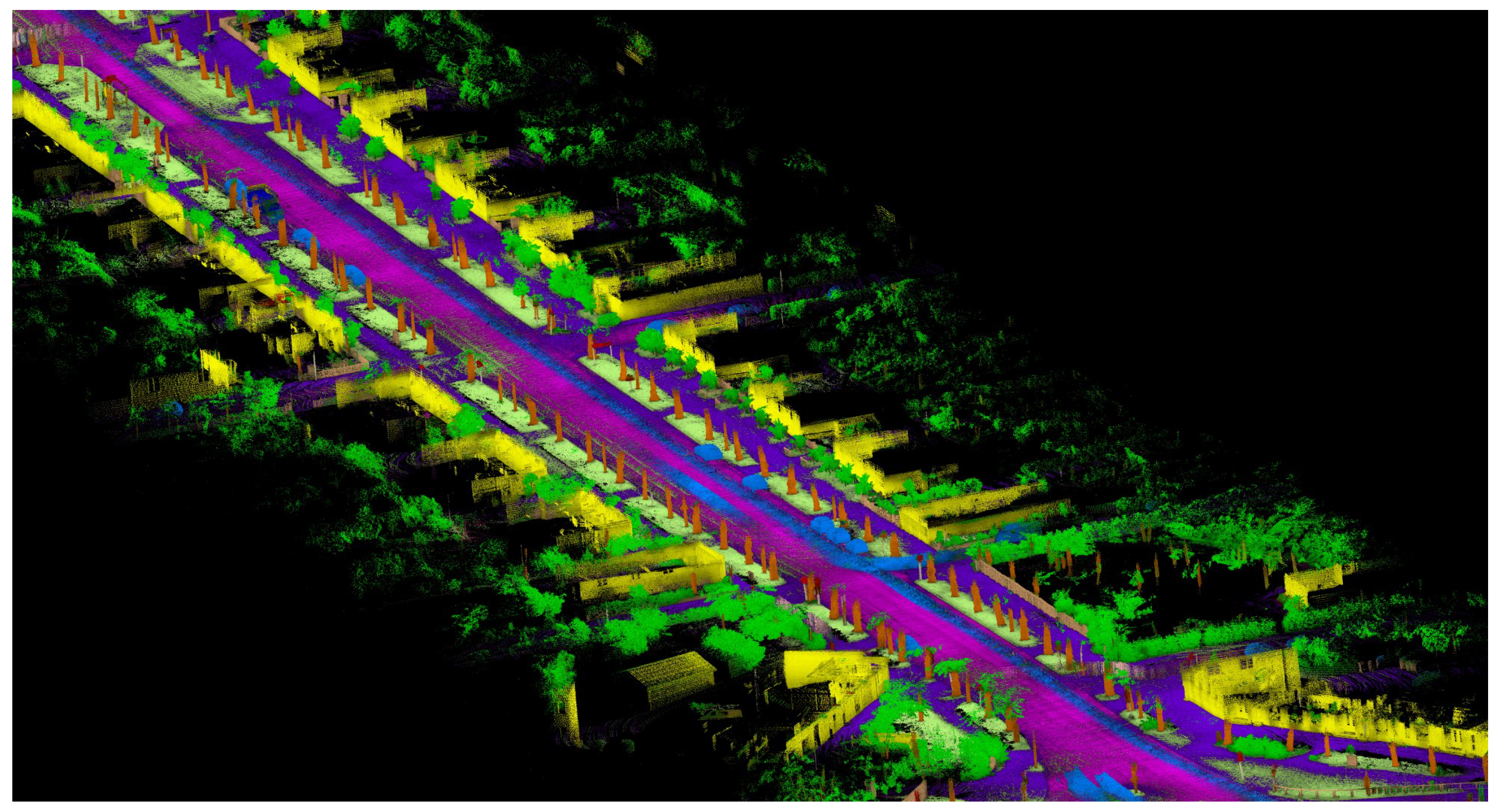
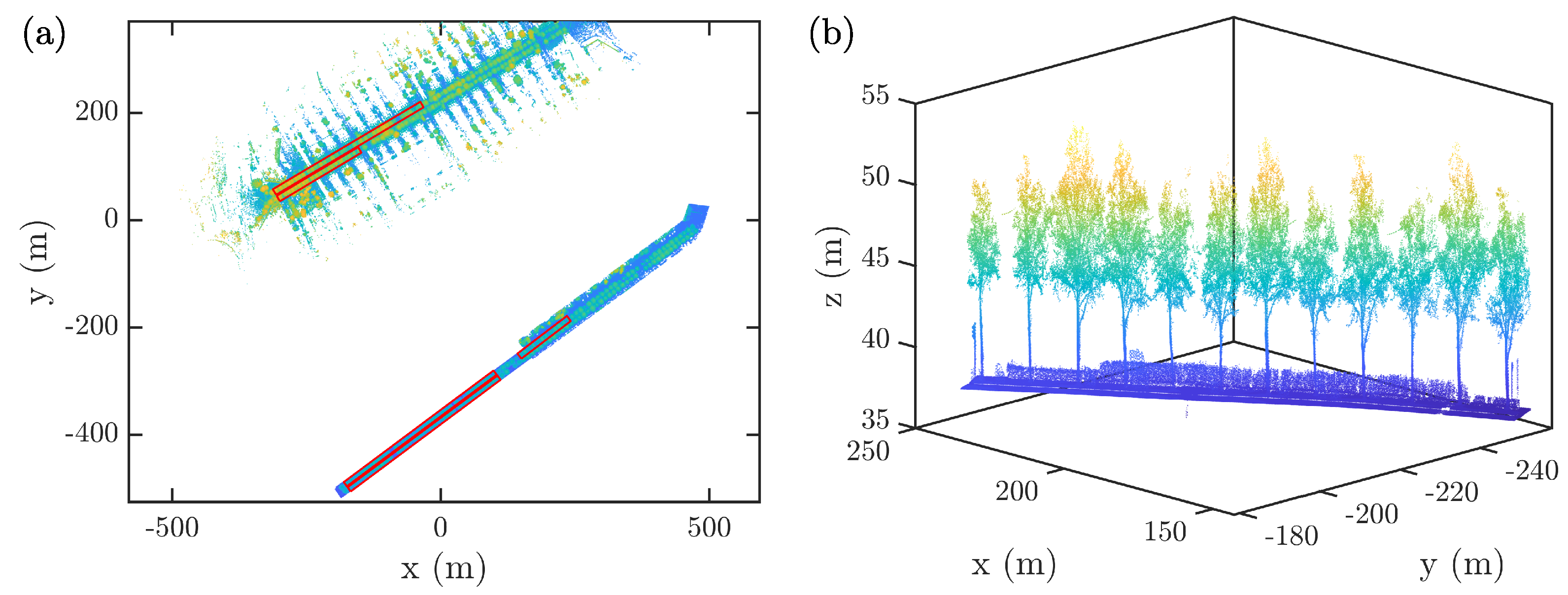
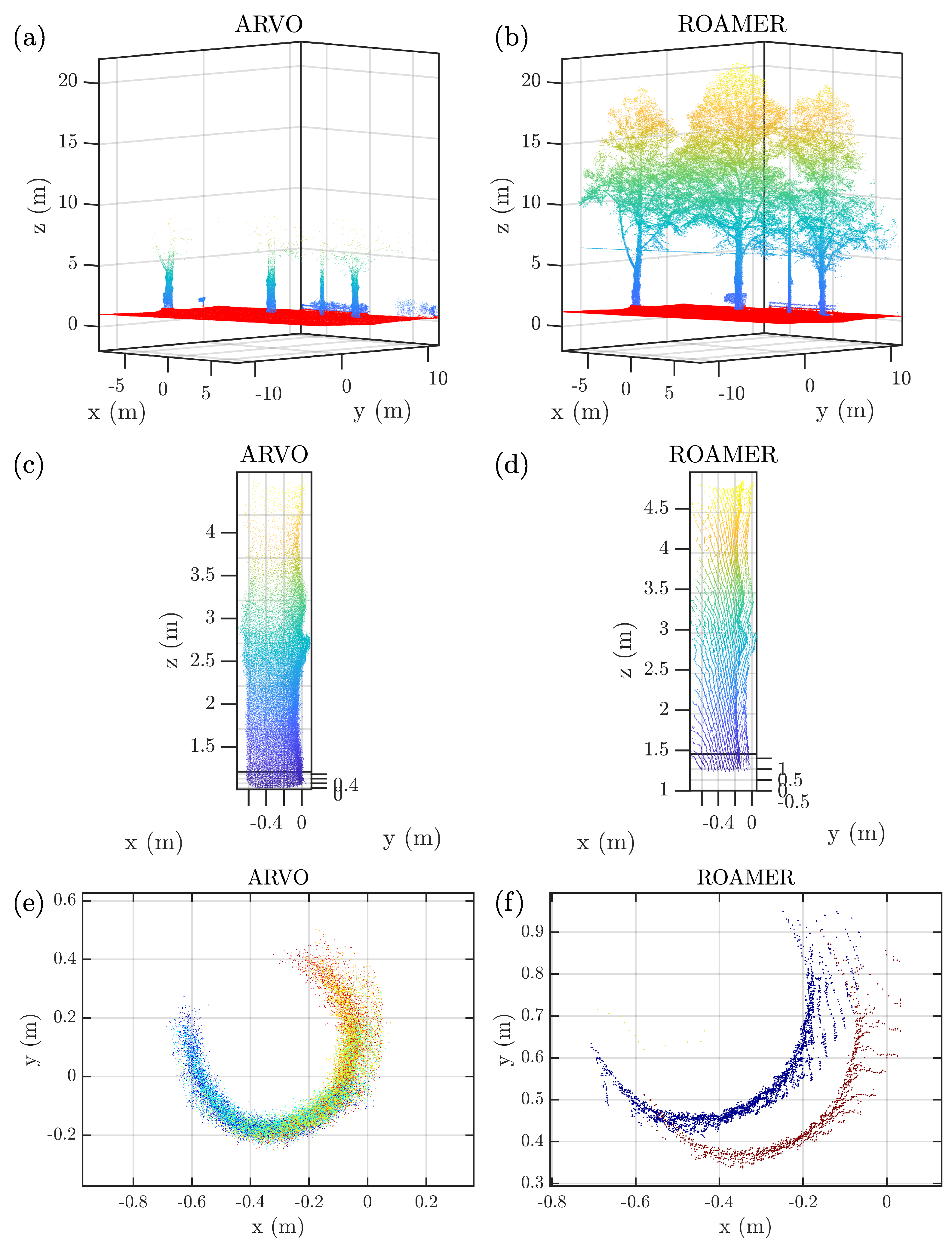
3.3.3. Cropping and Illustrating the Point Cloud Data

After processing the laser scanning data into point cloud format, we searched for all of the points that were located within five rectangular regions chosen to cover the 139 reference trees, as visualized in Figure 6a,b. The widths of the rectangular regions were set to 12 m, whereas their lengths were such that each reference tree was contained in exactly one of the regions. The points that were not contained in any of the rectangular regions were discarded in further point cloud-processing steps.

In Figure 7a,b, we visualize small sections of the point clouds obtained with the ARVO and ROAMER systems after the pre-processing steps. From Figure 7a, we see that the field of view of the laser scanner in the ARVO system limits us from modeling the tree crowns since the environment is captured in the point cloud with a reasonable point density only approximately up to the height of 5 m. This limitation is not present in the point cloud collected with the ROAMER system that can also accurately capture the tree tops. In Figure 7c–f, we illustrate the stem of an example tree in the point clouds collected with the ARVO and ROAMER systems. By comparing the horizontal cross-section of the tree trunk shown in Figure 7e,f, we see that the ranging accuracy of the laser scanner in the ROAMER system is better than that of the ARVO system. Note also that both of the point clouds suffer from distortions arising from the slow drift in the positioning of the laser scanner. For the example tree visualized in Figure 7c–f, the drift is more prominent for the ROAMER system point cloud because the points shown in Figure 7f correspond to a back-and-forth pass of the same tree within a long time span compared to the points in Figure 7e that were recorded within a single pass.

3.3.4. Digital Terrain Model Creation

First, we determine the digital terrain model (DTM) using a ground point extraction method designed for urban scenes [69]. In summary, the process of finding the DTM goes as follows: First, the point cloud is divided into voxels, and principal component analysis is applied for each of the voxels to estimate a flatness score describing how well the points in the voxel are approximated by a planar surface. Subsequently, voxels with a high flatness score and a close-to-vertical normal vector are used to find ground points by combining flat voxels with the help of surface growing and surface patch merging. After finding the ground points, the point cloud is divided into square-shaped pixels with a side length of 1 m in the $xy$ plane, and the ground elevation at each pixel is found by taking the median z-coordinate of the ground points located within each pixel. Finally, a Gaussian filter with a standard deviation of 1.5 m is applied to ensure the smoothness of the DTM. After estimating the DTM, the ground elevation is subtracted from the z-coordinate of each point in the point cloud.

3.3.5. Stem Curve and DBH Estimation

To detect trees and estimate their stem curves, we used an algorithmic workflow that was developed in [7] to enable accurate stem diameter measurements from MLS point clouds suffering from drifts in the trajectory of the laser scanner (see Figure 7f). We used heuristic criteria to slightly adjust the parameter values of the algorithms from those previously reported in [7] since the properties of the trees and the laser scanner systems studied in this work differ somewhat from those in the previous studies.

Table 2. The most important parameters for the stem curve estimation algorithm. In the table, MAD refers to the median absolute deviation that has been scaled, such that it estimates the same population quantity as the standard deviation in the case of the normal distribution.

Parameter	ARVO	ROAMER
Arc detection
Width of height interval in the z-direction (m)	0.2	0.2
Duration of time interval (s)	0.2	0.1
Neighborhood radius for DBSCAN (cm)	7.5	7.5
Point number threshold for DBSCAN	4	4
Outlier threshold in the radial direction for RANSAC (cm)	3.5	3.0
Minimum ratio of non-outlying points for RANSAC	0.75	0.75
Minimum number of points in arc	15	15
Maximum standard deviation of radial residuals in the arc (cm)	1.75	1.75
Minimum diameter of the arc (cm)	10.0	10.0
Maximum diameter of the arc (cm)	80.0	80.0
Minimum central angle of the arc (rad)	$0.6\pi$	$0.6\pi$
Clustering arcs into trees
Neighborhood radius for DBSCAN (cm)	50	50
Minimum number of arcs for DBSCAN	3	3
Minimum z difference between highest and lowest arc (m)	1.0	1.0
Detection of outlying diameter estimates
Number of nearest diameter estimates in the z-direction to use for comparison	5	5
Maximum of $|D\left(z_j\right)-\mathrm{median}\left(\{D\left(z_{j-2}\right),\dots ,D\left(z_{j+2}\right)\}\right)|/\mathrm{MAD}\left(\{D\left(z_{j-2}\right),\dots ,D\left(z_{j+2}\right)\}\right)$	2.0	2.0
Maximum of $|D\left(z_j\right)-\mathrm{median}\left(\{D\left(z_{j-2}\right),\dots ,D\left(z_{j+2}\right)\}\right)|$ (cm)	4.0	4.0
Largest allowed z difference between the nearest arcs (m)	4.0	4.0

summarizes the values of the most relevant parameters. Compared to previous studies using similar algorithms, we used a relatively small height interval width of 0.2 m because the tree diameters varied significantly as a function of elevation from the ground due to deformations in the tree trunks. On the other hand, we set the maximum standard deviation of radial residuals for arc detection to a higher value than in [7] to detect stem points of trees with relatively non-circular stems and to account for the higher noise in the point clouds. It should be noted that these parameters were not optimized to achieve optimal performance for the current dataset.

As the first step in the stem detection process, we aim to detect arc-shaped point groups that potentially correspond to the stems of trees. To achieve this, we divide the points in the point cloud into disjoint subsets based on their z-coordinate and time stamp. We use equispaced height intervals of 0.2 m and equispaced time intervals of 0.2 and 0.1 s for the ARVO and ROAMER systems, respectively. For each subset, we apply density-based clustering for applications with noise (DBSCAN) [70] to detect connected point groups that potentially correspond to stem arcs. Subsequently, we fit a circle to each DBSCAN cluster using the random sample consensus (RANSAC) framework [71]. The number of iterations for the RANSAC circle fitting is set as

$$N_{\mathrm{RANSAC}}=\frac{ln(1-0.99)}{ln(1-{\eta }_{\mathrm{in}}^3)},$$

(1)

where ln denotes the natural logarithm, and ${\eta }_{\mathrm{in}}$ is the minimum acceptable ratio of non-outlying points compared to all points. With the number of RANSAC iterations, we acquire at least one set of three non-outlying points for circle fitting with a probability of 99%, assuming an inlier ratio of ${\eta }_{\mathrm{in}}$.

Based on the RANSAC fit, we discard all clusters, for which the circular fit is poor, and we filter out possible noise points in the retained clusters. For the retained clusters, we subsequently fit a circle in the $xy$-plane using the numerically efficient and bias-free method described in Al-Sharadqah and Chernov (2009) [72]. The hyper-accurate circle fit corresponds to finding the eigenvector by minimizing the function ${\left|\right|\mathit{Z}\mathit{\beta }\left|\right|}_2^2={\mathit{\beta }}^T{\mathit{Z}}^T\mathit{Z}\mathit{\beta }$ for the following generalized eigenvalue problem

$${\mathit{Z}}^T\mathit{Z}\mathit{\beta }=\lambda \mathit{S}\mathit{\beta },$$

(2)

where the ith row of $\mathit{Z}$ reads ${\mathit{Z}}_{i:}={(x_i^2+y_i^2,x_i,y_i,1)}^T$, $\mathit{\beta }$ denotes a coefficient vector $\mathit{\beta }={(A,B,C,D)}^T$ associated with a circle $A(x^2+y^2)+Bx+Cy+D=0$, $\lambda$ denotes the generalized eigenvalue, and $\mathit{S}$ encodes the hyper-fit constraint that ensures a vanishing bias of the circle fit

$$\mathit{S}=\left(\begin{array}{cccc}8\overline{z}& 4\overline{x}& 4\overline{y}& 2\\ 4\overline{x}& 1& 0& 0\\ 4\overline{y}& 0& 1& 0\\ 2& 0& 0& 0\end{array}\right),$$

(3)

where $\overline{z}$ corresponds to the average value of the set ${\{x_i^2+y_i^2\}}_{i=1}^N$, and $\overline{x}$ and $\overline{y}$ are the average values of the x and y coordinates, respectively. Subsequently, the center and the radius R of the fitted circle $(x_0,y_0)$ can be inferred from the solved coefficient vector $\mathbf{\beta }$ as

$$x_0=-\frac{B}{2A},y_0=-\frac{C}{2A},R=\sqrt{\frac{B^2+C^2}{4A^2}-\frac{D}{A}}.$$

(4)

After circle fitting, the properties of each of the circular fits are compared to heuristically chosen quality criteria, such as the standard deviation of radial residuals and the central angle of the circular arc. See the section on arc detection in Table 2 for a full set of the quality criteria and their threshold values. The clusters satisfying the quality criteria are kept for further processing and regarded as stem arcs.

In the next step of the stem detection process, we apply DBSCAN clustering to the centers of the stem arcs to group the arcs further into tree trunks. For each of the resulting clusters, we calculate the height difference between the lowest and highest arc. We retain clusters with a height difference greater than 1 m, which are regarded as tree trunks. Next, we estimate the growth direction for each detected tree trunk using principal component analysis applied to the arc centers. This approach enables us to efficiently estimate the stem diameter by fitting a circle in the plane perpendicular to the growth direction. This mitigates errors in the stem diameter estimation arising from the inclination of trees. For each detected tree, the stem diameter is estimated at a height of $z=0.5\mathrm{m}+j\times 0.2$ m, where $j\ge 0$, using the iterative arc matching algorithm proposed in [73]. This algorithm alternates between fitting a circle with a fixed radius and a circle with a fixed center to the arcs of a tree within a given height interval to estimate the stem diameter at that height, while also providing a helpful visualization of the tree stem after correcting time-dependent distortions of the point cloud. The circle fitting is carried out in the plane perpendicular to the tree growth direction to eliminate diameter estimation errors arising from a non-vertical growth direction.

For each detected tree, outlying diameter estimates are then removed with the help of an automatic outlier detection scheme proposed in [73], which enables us to classify a diameter estimate $D_j$ at height $z_j$ as an outlying observation if it satisfies either of the two conditions:

• Find the $k=5$ nearest diameter estimates based on the height z (including the height interval itself), and compute the median (MEDIAN) and median absolute deviation (MAD) of these diameter values. If both of the following inequalities are fulfilled, the point $(z_j,D_j)$ is classified as an outlier

  (a)

  $|D_j-\mathrm{MEDIAN}|>2\times \mathrm{MAD}$,

  (b)

  $|D_j-\mathrm{MEDIAN}|>4.0$ cm.

• If the point is not included in the largest connected set of diameter estimates, it is regarded as an outlier. A set of diameter estimates is regarded as a connected set if all vertical distances between any consecutive diameter estimates sorted based on their z-value satisfy $|z_j-z_{j+1}|<4.0$ m.

The final estimate of the stem curve is obtained by fitting a cubic smoothing spline [74,75] to the retained diameter estimates. The value of the smoothing parameter is chosen using leave-one-out cross-validation from the interval $\lambda \in [0.001,0.05]$. The DBH is obtained by interpolating the smoothing spline at a height of $z=1.3$ m if the lowest stem diameter estimate is located below $z=1.3$ m. If the lowest stem diameter estimate is above $z=1.3$ m, the DBH is estimated by extrapolating the stem curve to the height of $z=1.3$ m using the approach described in [7]:

• If the stem curve is estimated from a height interval taller than 3.0 m, the DBH is computed by fitting a line to the lowest 3.0 m of the fitted smoothing spline and then extrapolating the line to $z=1.3$ m.
• If the stem curve is estimated from a height interval shorter than 3.0 m, a square root function $D\left(z\right)=D_0\sqrt{1-z/h}$, with h denoting the tree height, is fitted to the stem curve, and then evaluated at $z=1.3$ m to estimate the DBH.

3.4. Statistical Analysis

Here, we present the metrics that were applied to assess the accuracy of stem detection and stem diameter estimation from point clouds collected with the ARVO and ROAMER systems. Prior to computing the accuracy metrics, a mapping from the detected trees to the reference trees was established by finding the closest detected tree for each reference tree using a distance threshold of 1.25 m and, subsequently, inverting the mapping.

The success rate of stem detection was quantitatively judged using the concepts of completeness, i.e., recall, and correctness, i.e., precision, defined as [76]

$$\begin{array}{cc}\hfill \mathrm{Completeness}& =\frac{N_{\det },\mathrm{ref}}{N_{\mathrm{ref}}}\times 100\%,\hfill \end{array}$$

(5)

$$\begin{array}{cc}\hfill \mathrm{Correctness}& =\frac{N_{\det },\mathrm{ref}}{N_{\det }}\times 100\%,\hfill \end{array}$$

(6)

where $N_{\det },\mathrm{ref}$ denotes the number of detected reference trees, $N_{\mathrm{ref}}$ denotes the total number of reference trees, and $N_{\det }$ denotes the total number of detected objects regarded as trees.

The concepts of bias and root-mean-square error (RMSE) were applied to assess the accuracy of the obtained DBH estimates as

$$\begin{array}{cc}\hfill \mathrm{bias}& =\sum _{i=1}^{N_{\det },\mathrm{ref}}\frac{{\mathrm{DBH}}_i-{\mathrm{DBH}}_{i,\mathrm{ref}}}{N_{\det },\mathrm{ref}},\hfill \end{array}$$

(7)

$$\begin{array}{cc}\hfill \mathrm{RMSE}& =\sqrt{\sum _{i=1}^{N_{\det },\mathrm{ref}}\frac{{({\mathrm{DBH}}_i-{\mathrm{DBH}}_{i,\mathrm{ref}})}^2}{N_{\det },\mathrm{ref}}},\hfill \end{array}$$

(8)

where ${\left\{{\mathrm{DBH}}_i\right\}}_{i=1}^{N_{\det },\mathrm{ref}}$ denotes the DBH values of the detected reference trees estimated from the point cloud data, and ${\left\{{\mathrm{DBH}}_{i,\mathrm{ref}}\right\}}_{i=1}^{N_{\det },\mathrm{ref}}$ denotes the corresponding set of reference values obtained from the manual field measurements. Additionally, we calculated the relative bias and RMSE as follows

$$\begin{array}{cc}\hfill \mathrm{rbias}& =\frac{\mathrm{bias}}{\langle \mathrm{DBH}\rangle }\times 100\%,\hfill \end{array}$$

(9)

$$\begin{array}{cc}\hfill \mathrm{rRMSE}& =\frac{\mathrm{RMSE}}{\langle \mathrm{DBH}\rangle }\times 100\%,\hfill \end{array}$$

(10)

where $\langle \mathrm{DBH}\rangle ={\sum }_{i=1}^{N_{\det },\mathrm{ref}}{\mathrm{DBH}}_{i,\mathrm{ref}}/N_{\det },\mathrm{ref}$ denotes the mean of the reference DBH values.

For the estimated stem curves, we evaluated the individual bias and RMSE for each of the trees as well as the overall bias and RMSE for all of the trees. The bias and RMSE of the stem curve of the ith tree were computed as

$$\begin{array}{cc}\hfill {\mathrm{bias}}_i& =\sum _{j=1}^{N_i}\frac{D_i\left(z_j\right)-D_{i,\mathrm{ref}}\left(z_j\right)}{N_i},\hfill \end{array}$$

(11)

$$\begin{array}{cc}\hfill {\mathrm{RMSE}}_i& =\sqrt{\sum _{j=1}^{N_i}\frac{{(D_i\left(z_j\right)-D_{i,\mathrm{ref}}\left(z_j\right))}^2}{N_i}},\hfill \end{array}$$

(12)

where $D_i\left(z_j\right)$ is the stem diameter estimated from the point cloud for the ith tree at the height of $z_j$, $D_{i,\mathrm{ref}}\left(z_j\right)$ is the corresponding reference value of the diameter, and $N_i$ corresponds to the number of reference diameter estimates used for the computation. The relative bias and RMSE for the ith stem curve are obtained analogously to Equations (9) and (10) after normalization with the mean of the reference diameters, i.e., $\langle D_{i,\mathrm{ref}}\rangle ={\sum }_{j=1}^{N_i}{D}_{i,\mathrm{ref}}\left(z_j\right)/N_i$.

To estimate the overall bias and RMSE of stem curve estimates, we assign an equal weight for each of the trees and use Equations (11) and (12) to obtain

$$\begin{array}{cc}\hfill \mathrm{bias}& =\sum _{i=1}^{N_{\det },\mathrm{ref}}\frac{{\mathrm{bias}}_i}{N_{\det },\mathrm{ref}},\hfill \end{array}$$

(13)

$$\begin{array}{cc}\hfill \mathrm{RMSE}& =\sqrt{\sum _{i=1}^{N_{\det },\mathrm{ref}}\frac{{\mathrm{RMSE}}_i^2}{N_{\det },\mathrm{ref}}}.\hfill \end{array}$$

(14)

The overall relative bias and RMSE of the stem curve estimates are obtained analogously to Equations (9) and (10) after a normalization with the mean of the reference diameters, i.e., $\langle D_{\mathrm{ref}}\rangle =N_{\det },{\mathrm{ref}}^{-1}{\sum }_{i=1}^{N_{\det },\mathrm{ref}}{\sum }_{j=1}^{N_i}{D}_{i,\mathrm{ref}}\left(z_j\right)/N_i$.

4. Results

In this section, we present the results for the stem detection and stem diameter estimation using the autonomous perception data collected with the ARVO system. Furthermore, we present the corresponding results obtained with the ROAMER system, enabling us to compare the accuracies of the two systems and to further discuss the strengths and weaknesses of using autonomous perception data for updating the attributes of city trees. The key results for stem detection and stem curve estimation are summarized in

Table 3. Summary of the results regarding tree detection and stem diameter estimations for the ARVO and ROAMER systems. The table provides the completeness and correctness rates of tree detection as well as the bias and RMSE of DBH and stem curve estimates. For the bias and RMSE, we provide the relative value within the parentheses and the absolute value without parentheses. Note that the correctness rate refers to the value without performing any classification of the object type.

System	Completeness	Correctness	DBH		Stem Curve
			Bias	RMSE	Bias	RMSE
ARVO	96.4%	87.6%	2.1 cm (4.3%)	5.2 cm (10.4%)	2.3 cm (4.7%)	4.9 cm (10.2%)
ROAMER	100.0%	84.2%	−2.3 cm (−4.8%)	7.4 cm (15.0%)	−1.5 cm (−3.1%)	6.6 cm (14.0%)

.

4.1. Completeness and Correctness Related to Stem Detection

Using the automatic stem detection algorithm discussed in Section 3.3.5, we detected 134 of the 139 reference trees from the data collected with the autonomous ARVO system, and all of the 139 reference trees from the data collected with the mobile mapping system ROAMER. According to Equation (5), these values correspond to completeness rates of 96.4% and 100.0% for the ARVO and ROAMER systems, respectively. For both of the datasets, the automatic stem detection algorithm resulted in some false-positive detection events, in which a traffic sign or a pole was regarded as a tree trunk due to its cylindrical shape. The number of detected non-tree objects was 19 in the case of the ARVO system and 26 in the case of the ROAMER system, resulting in correctness rates of 87.6% and 84.2% for the ARVO and ROAMER systems, respectively. In principle, the non-tree objects can be filtered out at least partially by using existing object-level or point-level classification methods based on hand-selected features (e.g., [69]) or deep learning (e.g., [77]). Furthermore, the locations of the urban trees may be known a priori based on a tree register maintained by the city and, thus, it may be straightforward to discard the non-tree objects when updating the stem information of the urban trees tracked in the register.

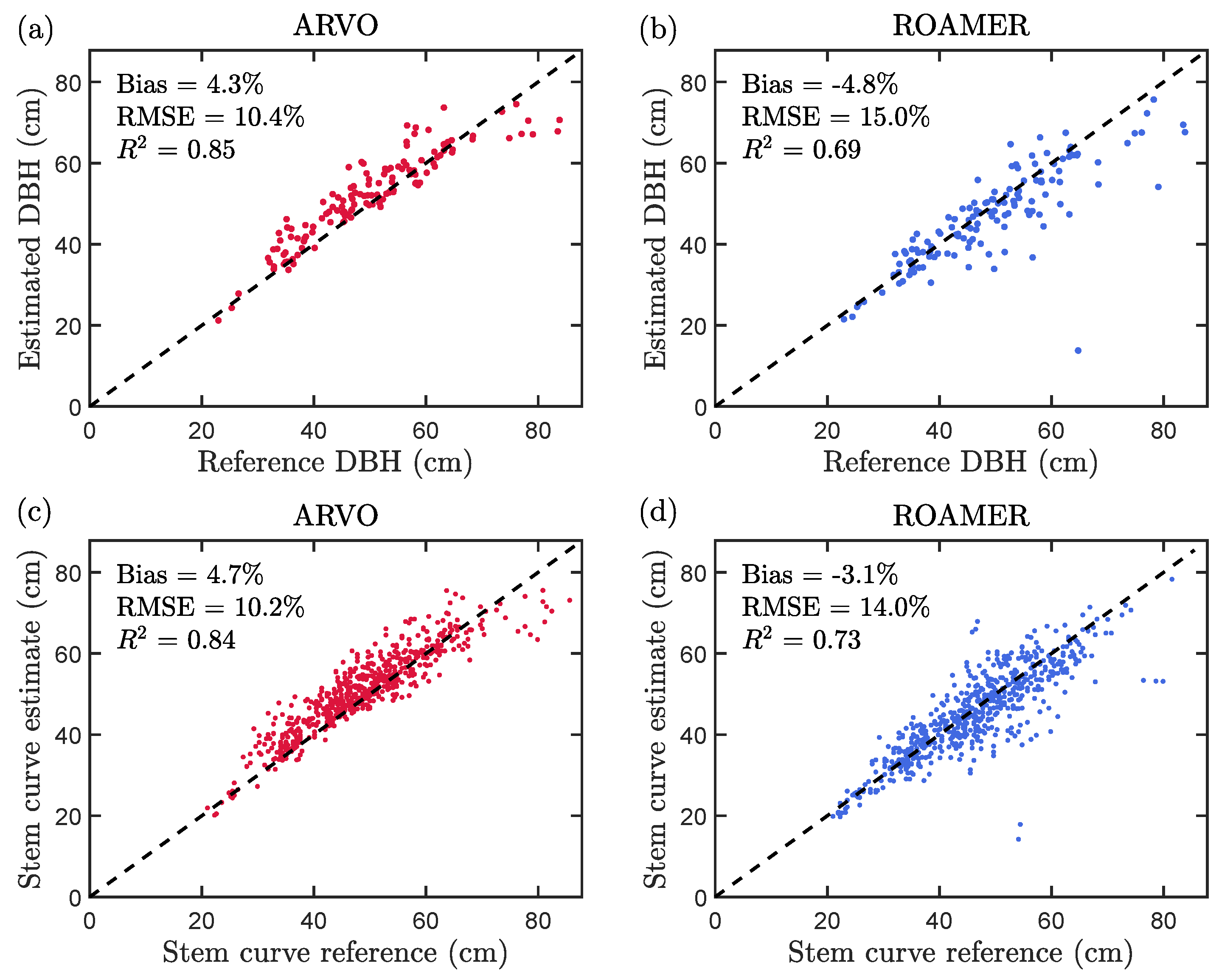
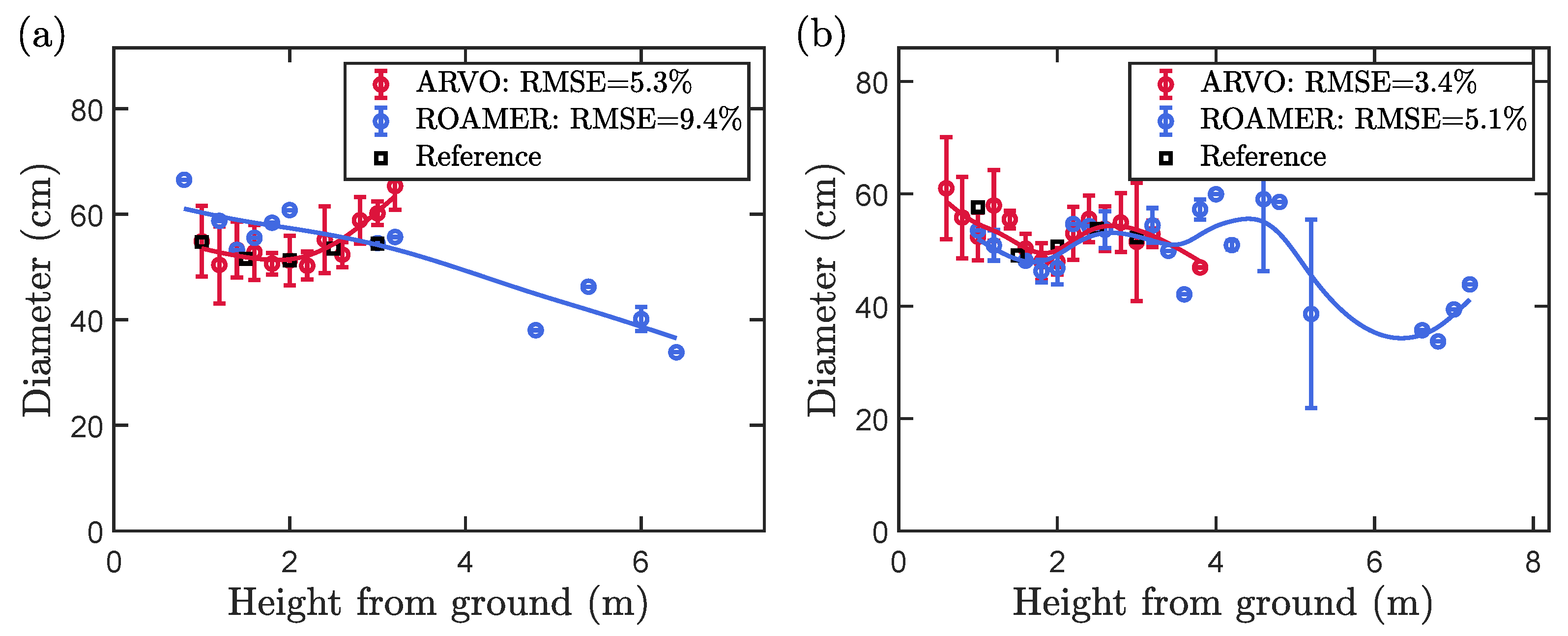
4.2. Accuracy Related to the Measured Stem Attributes

Here, we report the accuracy of the DBH and stem curve estimates obtained from the autonomous perception data that were collected using the ARVO system as well as the corresponding results obtained from the reference laser scanning dataset that was acquired using the ROAMER system. As illustrated in Figure 8a, the DBH estimates obtained using the ARVO system were associated with a bias of 2.1 cm, i.e., 4.3%, and a RMSE of 5.2 cm, i.e., 10.4%. When it comes to the ROAMER system, the corresponding statistical figures were $-2.3$ cm, i.e., $-4.8$% for the bias, and 7.4 cm, i.e., 15.0% for the RMSE, as visualized in Figure 8b.

In Figure 8c,d, we show scatter plots for the stem curve estimates acquired using the ARVO and ROAMER systems. For the ARVO system, the bias and RMSE of the stem curve estimates were 2.3 cm, i.e., 4.7%, and 4.9 cm, i.e., 10.2%, respectively. When it comes to the stem curve estimates obtained using the ROAMER system, the bias was $-1.5$ cm, i.e., $-3.1$%, whereas the RMSE was 6.6 cm, i.e., 14.0%. Thus, the accuracy of the stem curve estimation was virtually equivalent to the accuracy of the DBH estimation for both measurement systems. For both systems, the relative error in the stem curves of individual trees was below 10% for most of the trees, as illustrated by the histograms of the bias and RMSE values in Figure 9a,b. However, relative bias and RMSE values exceeding 20% were obtained for a small number of trees in the cases of both measurement systems.

Figure 9c,d illustrate the typical height range for successful stem curve estimation for the two measurement systems by showing histograms of the lowest and highest height at which the stem diameter could be accurately estimated using the algorithm described in Section 3.3.5. The mean of the lowest heights was slightly below 1.0 m for both systems, with 0.79 m for the ARVO system and 0.88 m for the ROAMER system. However, the ROAMER system allowed for stem curve estimation over a much wider height range, enabling the measurement of the stem curve up to an average height of 6.5 m. On the other hand, the ARVO system only enabled accurate stem diameter measurements up to an average height of 3.3 m. This difference is also exemplified in Figure 10a,b, which show two example stem curves obtained with the ARVO and ROAMER systems, respectively, along with the corresponding reference measurements. The ARVO system’s inability to provide stem diameter estimates above the height of 4.5 m is mainly due to the rapid reduction of point density as a function of height from the ground, as illustrated in Figure 11. The low point density for $z>5$ m mainly arises from the narrow field of view of the horizontally mounted VLS-128 scanner. It is worth noting that the ROAMER system has been designed for general mobile mapping applications, and therefore, its scanner has been chosen and mounted in a way that can capture the environment up to the height of treetops.

5. Discussion

In this section, we provide further discussion on the results obtained with the ARVO and ROAMER systems, and we also consider general guidelines for post-processing autonomous perception data while also listing various other potential applications of autonomous perception data for future research. Let us first discuss the reasons for obtaining a lower completeness rate of tree detection with the ARVO system when compared to the result obtained with the ROAMER system. The five trees, which were not detected from the data collected with the ARVO system, were visible in the point cloud, but they did not provide sufficiently many high-quality arcs that satisfied the quality criteria of the stem detection algorithm in Section 3.3.5 due to various reasons, such as a high number of deformations in the tree trunk or a highly non-circular stem shape. The completeness rate can be increased to 100% by reducing the strictness of the quality criteria for arc detection, e.g., by setting the minimum number of points in an arc to 10, the maximum standard deviation of radial residuals in an arc to 2.5 cm, and the minimum central angle of an arc to $0.45\pi$ rad. However, this has the consequence of increasing the number of unreliable arcs used for stem diameter estimation, which increases the root-mean-square error of the estimated stem diameters as discussed in [78]. The choice of parameters for stem detection depends on the specific application and the desired balance between the accuracy of the measured stem attributes and the success rate of tree detection.

Our case study showed that post-processing autonomous perception data enables us to estimate stem attributes of roadside trees with comparable or even slightly lower errors than those obtained with the ROAMER system designed for mobile mapping applications. We attribute the lower RMSE values obtained with the ARVO system to a few factors. Firstly, the measurements with the ROAMER system were conducted three growing seasons before the measurements with the ARVO system and four growing seasons before the manual field measurements. Thus, the tree trunks, especially their deformations (see Figure 1), may have grown and changed shapes during the time period of three years, potentially resulting in a slight overestimation of the reported error values of the ROAMER system. The overall growth of the stem diameters during 2017–2020 is reflected in the difference between the bias values obtained with the two systems, and it is not sufficient to explain the higher RMSE of the ROAMER system since the absolute values of the biases are approximately equal for the two systems.

Another reason why the ARVO system achieved a lower RMSE could be attributed to its use of a horizontal and forward-looking laser scanner providing a higher point density below the height of $z=3$ m and a better scanning angle for the task under study as compared with the ROAMER system. As a drawback of the narrow field of view of the forward-looking scanner (see Figure 11), we could not utilize the autonomous perception data to derive the tree height or the stem curve above the height of $z=4$ m when using the main scanner of the autonomous car. However, when using tilted VLP-16 scanners mounted on the sides of the car, we should be able to estimate the heights of the trees well. Since the mobile mapping ROAMER system had a better range accuracy, but higher errors in stem curve and DBH estimation, it can be concluded that the horizontally mounted scanner in the ARVO system was probably the main reason for obtaining lower errors in stem diameter estimation.

The RMSE values of 10–15% acquired in this work for the estimated stem diameters are somewhat higher than those obtained in previous studies using mobile laser scanning methodologies and similar algorithms for mapping pine-dominated boreal forests (e.g., [8,73]), where the RMSE of stem diameter estimation varied between 2% and 8%. Furthermore, some of the previous mobile laser scanning studies with roadside trees (e.g., [15,16,17]) reported RMSE values for the DBH ranging from 1 cm to approximately 4 cm corresponding to 14.0% with the average stem diameter in Forsman et al. (2016) [16]. We attribute the relatively high RMSE values obtained in this study to the irregular and non-cylindrical shapes of the tree stems, deformations in the tree trunks, and the thick and uneven bark of the trees (see Figure 1).

In the future, autonomous perception data collected with a setup similar to the ARVO system could be easily used for various other surveying and mapping applications, such as road rut and pothole detection, deriving building outlines visible from the road, collecting forest field references for forest inventories, texture mapping of buildings, deriving various pole-type objects, noise modeling, as well as other potential applications. However, each case should be studied separately since the quality of a point cloud obtained using the sensors of an autonomous vehicle is very different from that obtained with a designated mobile mapping system, such as ROAMER, due to the following reasons: (1) The viewing angles of the laser scanners are different, affecting object detection, for example, since most of the data comes from forward-looking scanners in the case of autonomous perception data, whereas designated mobile mapping systems often have scanners viewing approximately the direction perpendicular to the driving direction. (2) The use of forward-looking scanners in the collection of autonomous perception data means that the same part of an object can be visible in multiple scans, and the optimization and selection of view geometry have to be made. (3) In designated mobile mapping systems, the point cloud is often post-processed and registered in an accurate but computationally costly way, whereas autonomous perception data rely—by default—on real-time processing for tracking the trajectory of the scanner, e.g., using real-time SLAM-based approaches. This means that temporal drifts in the autonomous perception data may be significant and need to be accounted for when post-processing the data for mapping and surveying applications. This highlights the importance of saving the time stamp for each data point or saving the data points in temporal order such that one could afterward reduce drifts by computationally using more-involved SLAM algorithms or analyze the data by using algorithms based on temporal filtering. Note that temporal filtering was utilized in the stem diameter estimation algorithm in Section 3.3.5 by dividing the point cloud data into short time intervals. Time stamp information would be also useful for end users who aim to collect historic time-series using autonomous perception data.

Another highly important aspect for end-users is data access. The authors believe that autonomous car manufacturers and their networks aim to develop their own services based on autonomous perception data rather than sharing the data openly. Therefore, cities and organizations supporting the development of autonomous systems should understand this possibility and request any data, e.g., from a demo, in a format that allows mapping and surveying applications by post-processing the autonomous perception data. This area also calls for the standardization of data formats to enable post-processing-based surveying applications.

In the coming years, FGI is committed to sharing open data in this area, including publishing the necessary reference data to support the development of new applications related to autonomous big data analytics

6. Conclusions

In this paper, we demonstrated the potential of using autonomous perception data for mapping the roadside environment by considering the special case of measuring stem attributes of roadside trees, which could be used, e.g., to automatically update the tree register of a city. We showed that one of the most important tree parameters, diameter at breast height, could be estimated from autonomous perception data with a root-mean-square error of 10%, which was slightly lower than the corresponding error obtained from a specially-planned mobile mapping survey. The data processing workflow was optimized for the post-processing of autonomous perception data by using, e.g., time-based filtering in the algorithms applied for stem diameter estimation. Based on our findings, we expect that time stamp information may be important for achieving high accuracy in many applications of autonomous perception data. Furthermore, custom-made processing chains may need to be developed for each application using autonomous perception data due to the differences in the sensors and their arrangements compared to designated mobile mapping systems. For future research, we expect that a similar processing flow can be developed for various surveying and mapping applications, including road rut and pothole detection, building outline derivation, collecting forest field references for forest inventories, and the derivation of various pole-type objects.

References

1. Holland-Letz, D.; Kässer, M.; Kloss, B.; Müller, T. Mobility’s Future: An Investment Reality Check. 2021. Available online: https://www.mckinsey.com/industries/automotive-and-assembly/our-insights/mobilitys-future-an-investment-reality-check (accessed on 18 October 2022).
2. Rasshofer, R.H.; Gresser, K. Automotive radar and lidar systems for next generation driver assistance functions. Adv. Radio Sci. 2005, 3, 205–209. [Google Scholar] [CrossRef] [Green Version]
3. Kukko, A.; Kaijaluoto, R.; Kaartinen, H.; Lehtola, V.V.; Jaakkola, A.; Hyyppä, J. Graph SLAM correction for single scanner MLS forest data under boreal forest canopy. ISPRS J. Photogramm. Remote Sens. 2017, 132, 199–209. [Google Scholar] [CrossRef]
4. Karam, S.; Vosselman, G.; Peter, M.; Hosseinyalamdary, S.; Lehtola, V. Design, calibration, and evaluation of a backpack indoor mobile mapping system. Remote Sens. 2019, 11, 905. [Google Scholar] [CrossRef] [Green Version]
5. Lee, G.H.; Fraundorfer, F.; Pollefeys, M. Structureless pose-graph loop-closure with a multi-camera system on a self-driving car. In Proceedings of the 2013 IEEE/RSJ International Conference on Intelligent Robots and Systems, Tokyo, Japan, 3–7 November 2013; pp. 564–571. [Google Scholar]
6. Elhashash, M.; Albanwan, H.; Qin, R. A Review of Mobile Mapping Systems: From Sensors to Applications. Sensors 2022, 22, 4262. [Google Scholar] [CrossRef] [PubMed]
7. Hyyppä, E.; Hyyppä, J.; Hakala, T.; Kukko, A.; Wulder, M.A.; White, J.C.; Pyörälä, J.; Yu, X.; Wang, Y.; Virtanen, J.P.; et al. Under-canopy UAV laser scanning for accurate forest field measurements. ISPRS J. Photogr. Remote Sens. 2020, 164, 41–60. [Google Scholar] [CrossRef]
8. Hyyppä, E.; Yu, X.; Kaartinen, H.; Hakala, T.; Kukko, A.; Vastaranta, M.; Hyyppä, J. Comparison of Backpack, Handheld, Under-Canopy UAV, and Above-Canopy UAV Laser Scanning for Field Reference Data Collection in Boreal Forests. Remote Sens. 2020, 12, 3327. [Google Scholar] [CrossRef]
9. Li, Z.; Tan, J.; Liu, H. Rigorous boresight self-calibration of mobile and UAV LiDAR scanning systems by strip adjustment. Remote Sens. 2019, 11, 442. [Google Scholar] [CrossRef] [Green Version]
10. Seif, H.G.; Hu, X. Autonomous driving in the iCity—HD maps as a key challenge of the automotive industry. Engineering 2016, 2, 159–162. [Google Scholar] [CrossRef] [Green Version]
11. Al Najada, H.; Mahgoub, I. Autonomous vehicles safe-optimal trajectory selection based on big data analysis and predefined user preferences. In Proceedings of the 2016 IEEE 7th Annual Ubiquitous Computing, Electronics & Mobile Communication Conference (UEMCON), New York, NY, USA, 20–22 October 2016; pp. 1–6. [Google Scholar]
12. Virtanen, J.P.; Kukko, A.; Kaartinen, H.; Jaakkola, A.; Turppa, T.; Hyyppä, H.; Hyyppä, J. Nationwide point cloud—The future topographic core data. ISPRS Int. J. Geo-Inf. 2017, 6, 243. [Google Scholar] [CrossRef] [Green Version]
13. Jomrich, F.; Sharma, A.; Rückelt, T.; Burgstahler, D.; Böhnstedt, D. Dynamic Map Update Protocol for Highly Automated Driving Vehicles. In Proceedings of the 3rd International Conference on Vehicle Technology and Intelligent Transport Systems (VEHITS 2017), Porto, Portugal, 22–24 April 2017; pp. 68–78. [Google Scholar]
14. Xu, W.; Zhou, H.; Cheng, N.; Lyu, F.; Shi, W.; Chen, J.; Shen, X. Internet of vehicles in big data era. IEEE/CAA J. Autom. Sin. 2017, 5, 19–35. [Google Scholar] [CrossRef]
15. Wu, B.; Yu, B.; Yue, W.; Shu, S.; Tan, W.; Hu, C.; Huang, Y.; Wu, J.; Liu, H. A voxel-based method for automated identification and morphological parameters estimation of individual street trees from mobile laser scanning data. Remote Sens. 2013, 5, 584–611. [Google Scholar] [CrossRef] [Green Version]
16. Forsman, M.; Holmgren, J.; Olofsson, K. Tree stem diameter estimation from mobile laser scanning using line-wise intensity-based clustering. Forests 2016, 7, 206. [Google Scholar] [CrossRef] [Green Version]
17. Zhao, Y.; Hu, Q.; Li, H.; Wang, S.; Ai, M. Evaluating carbon sequestration and PM2. 5 removal of urban street trees using mobile laser scanning data. Remote Sens. 2018, 10, 1759. [Google Scholar] [CrossRef] [Green Version]
18. Ylijoki, O.; Porras, J. Perspectives to definition of big data: A mapping study and discussion. J. Innov. Manag. 2016, 4, 69–91. [Google Scholar] [CrossRef]
19. Laney, D. 3D data management: Controlling data volume, velocity and variety. META Group Res. Note 2001, 6, 1. [Google Scholar]
20. Mayer-Schönberger, V.; Cukier, K. Big Data: A Revolution that Will Transform How We Live, Work, and Think; Houghton Mifflin Harcourt: New York, NY, USA, 2013. [Google Scholar]
21. Rosenzweig, J.; Bartl, M. A review and analysis of literature on autonomous driving. E-J. Mak. Innov. 2015, 1–57. Available online: https://michaelbartl.com/ (accessed on 25 March 2023).
22. Jo, K.; Kim, C.; Sunwoo, M. Simultaneous localization and map change update for the high definition map-based autonomous driving car. Sensors 2018, 18, 3145. [Google Scholar] [CrossRef] [Green Version]
23. Van Brummelen, J.; O’Brien, M.; Gruyer, D.; Najjaran, H. Autonomous vehicle perception: The technology of today and tomorrow. Transp. Res. Part C Emerg. Technol. 2018, 89, 384–406. [Google Scholar] [CrossRef]
24. Liu, S.; Liu, L.; Tang, J.; Yu, B.; Wang, Y.; Shi, W. Edge computing for autonomous driving: Opportunities and challenges. Proc. IEEE 2019, 107, 1697–1716. [Google Scholar] [CrossRef]
25. Montanaro, U.; Dixit, S.; Fallah, S.; Dianati, M.; Stevens, A.; Oxtoby, D.; Mouzakitis, A. Towards connected autonomous driving: Review of use-cases. Veh. Syst. Dyn. 2019, 57, 779–814. [Google Scholar] [CrossRef]
26. Fujiyoshi, H.; Hirakawa, T.; Yamashita, T. Deep learning-based image recognition for autonomous driving. IATSS Res. 2019, 43, 244–252. [Google Scholar] [CrossRef]
27. Liu, L.; Lu, S.; Zhong, R.; Wu, B.; Yao, Y.; Zhang, Q.; Shi, W. Computing systems for autonomous driving: State of the art and challenges. IEEE Internet Things J. 2020, 8, 6469–6486. [Google Scholar] [CrossRef]
28. Ilci, V.; Toth, C. High definition 3D map creation using GNSS/IMU/LiDAR sensor integration to support autonomous vehicle navigation. Sensors 2020, 20, 899. [Google Scholar] [CrossRef] [Green Version]
29. Wong, K.; Gu, Y.; Kamijo, S. Mapping for autonomous driving: Opportunities and challenges. IEEE Intell. Transp. Syst. Mag. 2020, 13, 91–106. [Google Scholar] [CrossRef]
30. Yurtsever, E.; Lambert, J.; Carballo, A.; Takeda, K. A survey of autonomous driving: Common practices and emerging technologies. IEEE Access 2020, 8, 58443–58469. [Google Scholar] [CrossRef]
31. Pannen, D.; Liebner, M.; Hempel, W.; Burgard, W. How to keep HD maps for automated driving up to date. In Proceedings of the 2020 IEEE International Conference on Robotics and Automation (ICRA), Paris, France, 31 May–31 August 2020; pp. 2288–2294. [Google Scholar]
32. Mozaffari, S.; Al-Jarrah, O.Y.; Dianati, M.; Jennings, P.; Mouzakitis, A. Deep learning-based vehicle behavior prediction for autonomous driving applications: A review. IEEE Trans. Intell. Transp. Syst. 2020, 23, 33–47. [Google Scholar] [CrossRef]
33. Fayyad, J.; Jaradat, M.A.; Gruyer, D.; Najjaran, H. Deep learning sensor fusion for autonomous vehicle perception and localization: A review. Sensors 2020, 20, 4220. [Google Scholar] [CrossRef] [PubMed]
34. Badue, C.; Guidolini, R.; Carneiro, R.V.; Azevedo, P.; Cardoso, V.B.; Forechi, A.; Jesus, L.; Berriel, R.; Paixao, T.M.; Mutz, F.; et al. Self-driving cars: A survey. Expert Syst. Appl. 2021, 165, 113816. [Google Scholar] [CrossRef]
35. Yeong, D.J.; Velasco-Hernandez, G.; Barry, J.; Walsh, J. Sensor and sensor fusion technology in autonomous vehicles: A review. Sensors 2021, 21, 2140. [Google Scholar] [CrossRef]
36. Lin, X.; Wang, F.; Yang, B.; Zhang, W. Autonomous vehicle localization with prior visual point cloud map constraints in GNSS-challenged environments. Remote Sens. 2021, 13, 506. [Google Scholar] [CrossRef]
37. Feng, D.; Harakeh, A.; Waslander, S.L.; Dietmayer, K. A review and comparative study on probabilistic object detection in autonomous driving. IEEE Trans. Intell. Transp. Syst. 2021, 23, 9961–9980. [Google Scholar] [CrossRef]
38. Wang, M.; Chen, Q.; Fu, Z. Lsnet: Learned sampling network for 3d object detection from point clouds. Remote Sens. 2022, 14, 1539. [Google Scholar] [CrossRef]
39. Chalvatzaras, A.; Pratikakis, I.; Amanatiadis, A.A. A Survey on Map-Based Localization Techniques for Autonomous Vehicles. IEEE Trans. Intell. Veh. 2023, 8, 1574–1596. [Google Scholar] [CrossRef]
40. Geiger, A.; Lenz, P.; Stiller, C.; Urtasun, R. Vision meets robotics: The kitti dataset. Int. J. Robot. Res. 2013, 32, 1231–1237. [Google Scholar] [CrossRef] [Green Version]
41. Pham, Q.H.; Sevestre, P.; Pahwa, R.S.; Zhan, H.; Pang, C.H.; Chen, Y.; Mustafa, A.; Chandrasekhar, V.; Lin, J. A*3D dataset: Towards autonomous driving in challenging environments. In Proceedings of the 2020 IEEE International Conference on Robotics and Automation (ICRA), Paris, France, 31 May–31 August 2020; pp. 2267–2273. [Google Scholar]
42. Caesar, H.; Bankiti, V.; Lang, A.H.; Vora, S.; Liong, V.E.; Xu, Q.; Krishnan, A.; Pan, Y.; Baldan, G.; Beijbom, O. nuScenes: A multimodal dataset for autonomous driving. In Proceedings of the IEEE/CVF Conference on Computer Vision and Pattern Recognition, Seattle, WA, USA, 13–19 June 2020; pp. 11621–11631. [Google Scholar]
43. Sun, P.; Kretzschmar, H.; Dotiwalla, X.; Chouard, A.; Patnaik, V.; Tsui, P.; Guo, J.; Zhou, Y.; Chai, Y.; Caine, B.; et al. Scalability in perception for autonomous driving: Waymo open dataset. In Proceedings of the IEEE/CVF Conference on Computer Vision and Pattern Recognition, Seattle, WA, USA, 13–19 June 2020; pp. 2446–2454. [Google Scholar]
44. Huang, X.; Cheng, X.; Geng, Q.; Cao, B.; Zhou, D.; Wang, P.; Lin, Y.; Yang, R. The ApolloScape dataset for autonomous driving. In Proceedings of the 2018 IEEE/CVF Conference on Computer Vision and Pattern Recognition Workshops (CVPRW), Salt Lake City, UT, USA, 18–22 June 2018; pp. 954–960. [Google Scholar]
45. Geyer, J.; Kassahun, Y.; Mahmudi, M.; Ricou, X.; Durgesh, R.; Chung, A.S.; Hauswald, L.; Pham, V.H.; Mühlegg, M.; Dorn, S.; et al. A2d2: Audi autonomous driving dataset. arXiv 2020, arXiv:2004.06320. [Google Scholar]
46. Masello, L.; Sheehan, B.; Murphy, F.; Castignani, G.; McDonnell, K.; Ryan, C. From traditional to autonomous vehicles: A systematic review of data availability. Transp. Res. Rec. 2022, 2676, 161–193. [Google Scholar] [CrossRef]
47. Manninen, P.; Hyyti, H.; Kyrki, V.; Maanpää, J.; Taher, J.; Hyyppä, J. Towards High-Definition Maps: A Framework Leveraging Semantic Segmentation to Improve NDT Map Compression and Descriptivity. In Proceedings of the 2022 IEEE/RSJ International Conference on Intelligent Robots and Systems (IROS), Kyoto, Japan, 23–27 October 2022; pp. 5370–5377. [Google Scholar]
48. Daniel, A.; Subburathinam, K.; Paul, A.; Rajkumar, N.; Rho, S. Big autonomous vehicular data classifications: Towards procuring intelligence in ITS. Veh. Commun. 2017, 9, 306–312. [Google Scholar] [CrossRef]
49. Yoo, A.; Shin, S.; Lee, J.; Moon, C. Implementation of a sensor big data processing system for autonomous vehicles in the C-ITS environment. Appl. Sci. 2020, 10, 7858. [Google Scholar] [CrossRef]
50. Wang, H.; Feng, J.; Li, K.; Chen, L. Deep understanding of big geospatial data for self-driving: Data, technologies, and systems. Future Gener. Comput. Syst. 2022, 137, 146–163. [Google Scholar] [CrossRef]
51. Zhu, L.; Yu, F.R.; Wang, Y.; Ning, B.; Tang, T. Big data analytics in intelligent transportation systems: A survey. IEEE Trans. Intell. Transp. Syst. 2018, 20, 383–398. [Google Scholar] [CrossRef]
52. Hyyppä, J.; Kukko, A.; Kaartinen, H.; Matikainen, L.; Lehtomäki, M. SOHJOA-Projekti: Robottibussi Suomen Urbaaneissa Olosuhteissa; Metropolia Ammattikorkeakoulu: Helsinki, Finland, 2018; pp. 65–73. [Google Scholar]
53. Maanpää, J.; Taher, J.; Manninen, P.; Pakola, L.; Melekhov, I.; Hyyppä, J. Multimodal end-to-end learning for autonomous steering in adverse road and weather conditions. In Proceedings of the 2020 25th International Conference on Pattern Recognition (ICPR), Milan, Italy, 10–15 January 2021; pp. 699–706. [Google Scholar]
54. Maanpää, J.; Melekhov, I.; Taher, J.; Manninen, P.; Hyyppä, J. Leveraging Road Area Semantic Segmentation with Auxiliary Steering Task. In Proceedings of the Image Analysis and Processing–ICIAP 2022: 21st International Conference, Lecce, Italy, 23–27 May 2022; Proceedings Part I; Springer: Cham, Switzerland, 2022; pp. 727–738. [Google Scholar]
55. Taher, J.; Hakala, T.; Jaakkola, A.; Hyyti, H.; Kukko, A.; Manninen, P.; Maanpää, J.; Hyyppä, J. Feasibility of hyperspectral single photon LiDAR for robust autonomous vehicle perception. Sensors 2022, 22, 5759. [Google Scholar] [CrossRef]
56. Velodyne. VLP-16 Puck LITE, 2018. 63-9286 Rev-H Datasheet. Available online: https://www.mapix.com/wp-content/uploads/2018/07/63-9286_Rev-H_Puck-LITE_Datasheet_Web.pdf (accessed on 25 March 2023).
57. Velodyne. VLS-128 Alpha Puck, 2019. 63-9480 Rev-3 datasheet. Available online: https://www.hypertech.co.il/wp-content/uploads/2016/05/63-9480_Rev-3_Alpha-Puck_Datasheet_Web.pdf (accessed on 25 March 2023).
58. Novatel. PwrPak7-E1. 2020. Available online: https://novatel.com/products/receivers/enclosures/pwrpak7 (accessed on 25 March 2023).
59. Quigley, M.; Gerkey, B.; Conley, K.; Faust, J.; Foote, T.; Leibs, J.; Berger, E.; Wheeler, R.; Ng, A. ROS: An open-source Robot Operating System. In Proceedings of the ICRA Workshop on Open Source Software in Robotics, Kobe, Japan, 12–17 May 2009. [Google Scholar]
60. Hu, Q.; Yang, B.; Xie, L.; Rosa, S.; Guo, Y.; Wang, Z.; Trigoni, N.; Markham, A. RandLA-Net: Efficient semantic segmentation of large-scale point clouds. In Proceedings of the IEEE/CVF Conference on Computer Vision and Pattern Recognition (CVPR), Seattle, WA, USA, 13–19 June 2020; pp. 11108–11117. [Google Scholar]
61. El Issaoui, A.; Feng, Z.; Lehtomäki, M.; Hyyppä, E.; Hyyppä, H.; Kaartinen, H.; Kukko, A.; Hyyppä, J. Feasibility of mobile laser scanning towards operational accurate road rut depth measurements. Sensors 2021, 21, 1180. [Google Scholar] [CrossRef] [PubMed]
62. Holopainen, M.; Vastaranta, M.; Kankare, V.; Hyyppä, H.; Vaaja, M.; Hyyppä, J.; Liang, X.; Litkey, P.; Yu, X.; Kaartinen, H.; et al. The use of ALS, TLS and VLS measurements in mapping and monitoring urban trees. In Proceedings of the 2011 Joint Urban Remote Sensing Event, Munich, Germany, 11–13 April 2011; pp. 29–32. [Google Scholar]
63. Kukko, A.; Kaartinen, H.; Hyyppä, J.; Chen, Y. Multiplatform mobile laser scanning: Usability and performance. Sensors 2012, 12, 11712–11733. [Google Scholar] [CrossRef] [Green Version]
64. Kaartinen, H.; Hyyppä, J.; Kukko, A.; Jaakkola, A.; Hyyppä, H. Benchmarking the performance of mobile laser scanning systems using a permanent test field. Sensors 2012, 12, 12814–12835. [Google Scholar] [CrossRef] [Green Version]
65. Vaaja, M.; Hyyppä, J.; Kukko, A.; Kaartinen, H.; Hyyppä, H.; Alho, P. Mapping topography changes and elevation accuracies using a mobile laser scanner. Remote Sens. 2011, 3, 587–600. [Google Scholar] [CrossRef] [Green Version]
66. Jaakkola, A.; Hyyppä, J.; Hyyppä, H.; Kukko, A. Retrieval algorithms for road surface modelling using laser-based mobile mapping. Sensors 2008, 8, 5238–5249. [Google Scholar] [CrossRef] [Green Version]
67. Lehtomäki, M.; Jaakkola, A.; Hyyppä, J.; Kukko, A.; Kaartinen, H. Detection of vertical pole-like objects in a road environment using vehicle-based laser scanning data. Remote Sens. 2010, 2, 641–664. [Google Scholar] [CrossRef] [Green Version]
68. Novatel. Inertial Explorer, 2020. D18034 Version 9 brochure. Available online: https://www.amtechs.co.jp/product/Waypoint_D18034_v9.pdf (accessed on 25 March 2023).
69. Lehtomäki, M.; Jaakkola, A.; Hyyppä, J.; Lampinen, J.; Kaartinen, H.; Kukko, A.; Puttonen, E.; Hyyppä, H. Object classification and recognition from mobile laser scanning point clouds in a road environment. IEEE Trans. Geosci. Remote Sens. 2016, 54, 1226–1239. [Google Scholar] [CrossRef] [Green Version]
70. Ester, M.; Kriegel, H.P.; Sander, J.; Xu, X. A density-based algorithm for discovering clusters in large spatial databases with noise. In Proceedings of the Second International Conference on Knowledge Discovery and Data Mining (KDD’96), Portland, OR, USA, 2–4 August 1996; pp. 226–231. [Google Scholar]
71. Fischler, M.A.; Bolles, R.C. Random sample consensus: A paradigm for model fitting with applications to image analysis and automated cartography. Commun. ACM 1981, 24, 381–395. [Google Scholar] [CrossRef]
72. Al-Sharadqah, A.; Chernov, N. Error analysis for circle fitting algorithms. Electron. J. Stat. 2009, 3, 886–911. [Google Scholar] [CrossRef]
73. Hyyppä, E.; Kukko, A.; Kaijaluoto, R.; White, J.C.; Wulder, M.A.; Pyörälä, J.; Liang, X.; Yu, X.; Wang, Y.; Kaartinen, H.; et al. Accurate derivation of stem curve and volume using backpack mobile laser scanning. ISPRS J. Photogramm. Remote Sens. 2020, 161, 246–262. [Google Scholar] [CrossRef]
74. Pollock, D.S.G. Smoothing with Cubic Splines; Queen Mary University of London, School of Economics and Finance: London, UK, 1993. [Google Scholar]
75. De Boor, C. A Practical Guide to Splines; Springer: New York, NY, USA, 1978; Volume 27. [Google Scholar]
76. Liang, X.; Kukko, A.; Hyyppä, J.; Lehtomäki, M.; Pyörälä, J.; Yu, X.; Kaartinen, H.; Jaakkola, A.; Wang, Y. In-situ measurements from mobile platforms: An emerging approach to address the old challenges associated with forest inventories. ISPRS J. Photogramm. Remote Sens. 2018, 143, 97–107. [Google Scholar] [CrossRef]
77. Behley, J.; Garbade, M.; Milioto, A.; Quenzel, J.; Behnke, S.; Stachniss, C.; Gall, J. Semantickitti: A dataset for semantic scene understanding of lidar sequences. In Proceedings of the IEEE/CVF International Conference on Computer Vision, Seoul, Republic of Korea, 27–28 October 2019; pp. 9297–9307. [Google Scholar]
78. Hyyppä, E.; Kukko, A.; Kaartinen, H.; Yu, X.; Muhojoki, J.; Hakala, T.; Hyyppä, J. Direct and automatic measurements of stem curve and volume using a high-resolution airborne laser scanning system. Sci. Remote Sens. 2022, 5, 100050. [Google Scholar] [CrossRef]
Figure 1. (ac) Photographs of three example roadside trees located in the test area.
Remotesensing 15 01790 g001
Figure 2. Photograph of the autonomous mapping and driving research platform, ARVO, which was used to record the autonomous perception data in this study. The inset shows the trunk of the ARVO car.
Remotesensing 15 01790 g002
Figure 3. An illustration of point cloud data recorded with the ARVO system. This visualization uses semantic segmentation [60] and excludes the highest rings to make the road-level view and tree trunks (brown) more visible.
Remotesensing 15 01790 g003
Figure 4. ROAMER R3 mobile laser scanning system installed on top of a truss structure mounted on a car.
Remotesensing 15 01790 g004
Figure 5. Flow chart of the data processing steps utilized to detect roadside trees and to estimate their stem curves and DBHs.
Remotesensing 15 01790 g005
Figure 6. (a) Top view of the point cloud collected with the ROAMER system on Pohjolankatu and Koskelantie, together with the five rectangular regions (red lines) containing reference trees. For tree detection and stem diameter estimation, we retained the points located inside the red-colored rectangular regions that covered all 139 reference trees. (b) Side view of the point cloud collected with the ROAMER system within the shortest reference region on Koskelantie. In both panels, the points are colored based on the z-coordinates; the x y -coordinates of the points are centered by the mean value of the panel (a).
Remotesensing 15 01790 g006
Figure 7. (a,b) A small section of the point cloud collected using (a) the ARVO system, and (b) the ROAMER system. The points are colored based on their z-coordinates, apart from the ground points that are denoted in red. (c,d) Close-up of an example tree trunk in the point cloud collected using (c) the ARVO system, and (d) the ROAMER system. Again, the points are colored based on their z-coordinates. (e,f) Cross-sectional view of the tree trunk illustrated in panels (c,d), respectively, when considering points from the height interval z [ 1.5 , 2.5 ] m. The points are colored based on the acquisition time of the data, such that the blue color denotes an earlier time and the red color denotes a later time.
Remotesensing 15 01790 g007
Figure 8. (a) Scatter plot for the DBH estimates measured from the point cloud data collected using the ARVO system vs. the reference DBH values. (b) The same as (a) but for the DBH estimates measured from the point cloud data collected using the ROAMER system. (c) Scatter plot for the stem curve estimates measured from the point cloud data collected using the ARVO system vs. the reference values of the stem curves. (d) The same as (c) but for the stem curve estimates assessed from the point cloud data collected using the ROAMER system.
Remotesensing 15 01790 g008
Figure 9. (a) Histogram for the relative bias values of the measured stem curves based on Equation (11). (b) Histogram for the relative RMSE values of the measured stem curves based on Equation (12). In panels (a,b), we removed a single outlying stem curve measurement ( bias = 70.4 % , RMSE = 70.5 % ) obtained using the ROAMER system in order to better illustrate the overall distribution of the relative bias and RMSE values. (c) Histogram showing the distribution of the lowest height, at which the stem diameter could be estimated for each of the detected trees. (d) Histogram showing the distribution of the highest height, in which the stem diameter could be estimated for each of the detected trees. In all of the panels, the red bars correspond to estimates obtained using the ARVO system, whereas the blue bars denote the results acquired using the ROAMER system.
Remotesensing 15 01790 g009
Figure 10. (a) A stem curve estimated for an example tree using the ARVO (red dots) and ROAMER systems (blue dots) together with the reference values of the stem diameter based on manual measurements (black squares). The solid lines show the smoothing spline fits the individual stem diameter measurements. The error bars correspond to the standard deviation of the diameters of the detected arcs in each height interval. The relative RMSE values for the stem curve estimate are 3.4% and 5.1% for the ARVO and ROAMER systems, respectively. (b) The same as (a) but for another tree. The RMSE values for the stem curve estimates are 5.3% and 9.4% for the ARVO and ROAMER systems, respectively.
Remotesensing 15 01790 g010
Figure 11. Average point density for height intervals with a width of Δ z = 0.5 m as a function of the height from the ground level. The red (blue) curve denotes the point density within the point cloud data collected using the ARVO (ROAMER) system. Note the logarithmic scale on the y-axis.
Remotesensing 15 01790 g011