
Towards Prediction and Mapping of Grassland Aboveground Biomass Using Handheld LiDAR

 , and
, and
Abstract
1. Introduction
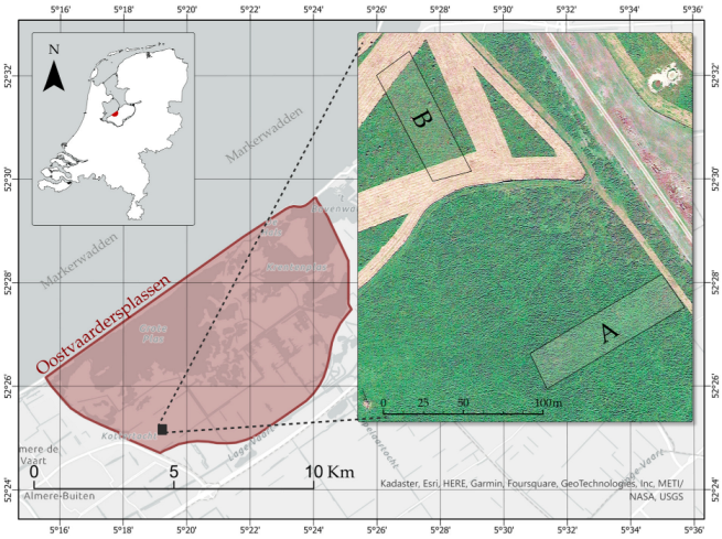
2. Study Area
3. Materials and Methods
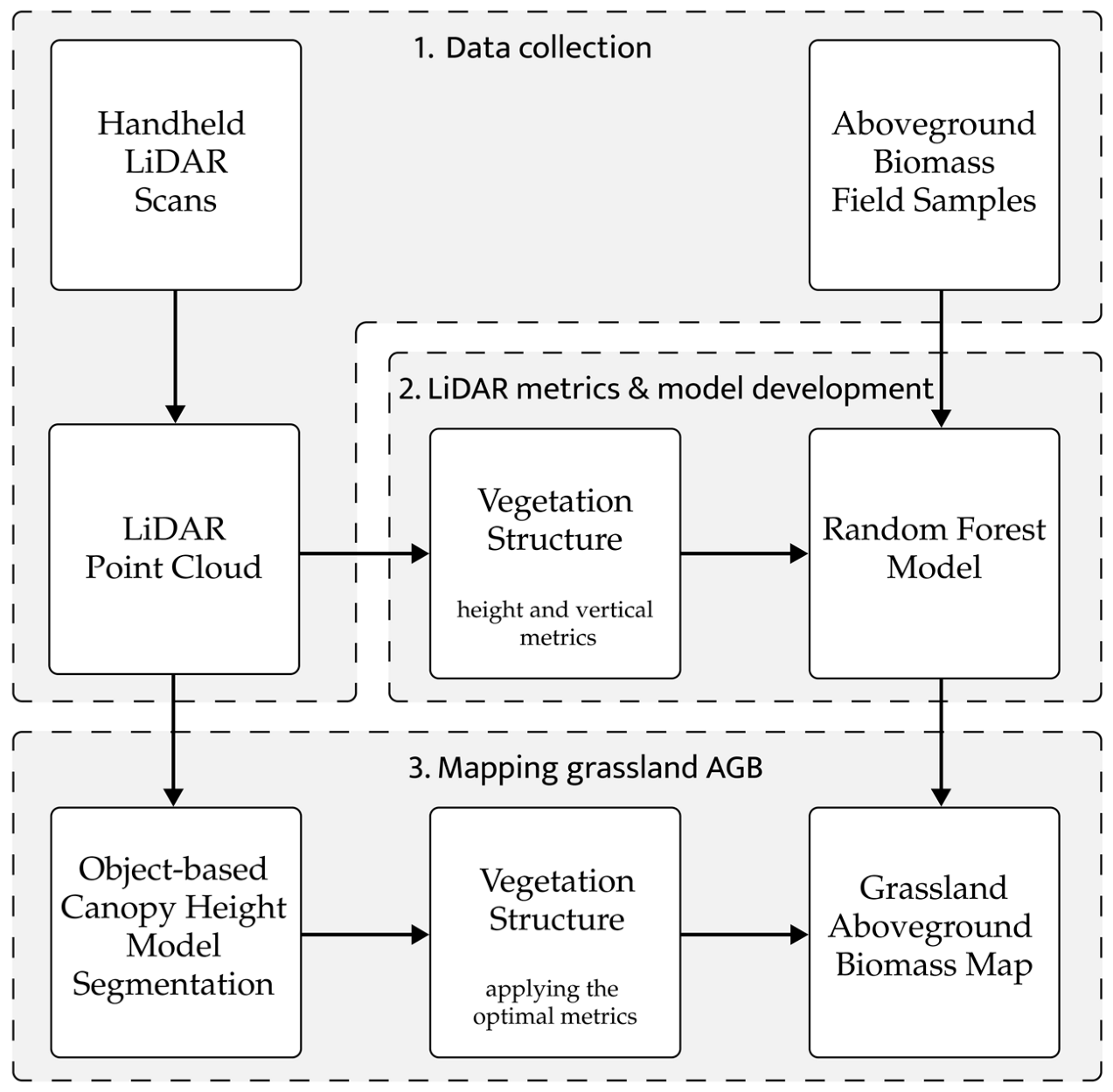
3.1. General Workflow
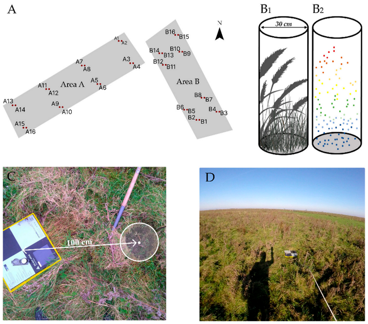
3.2. Data Collection
3.3. LiDAR Metrics and Model Development
3.4. Mapping Grassland AGB
3.5. Validation
4. Results
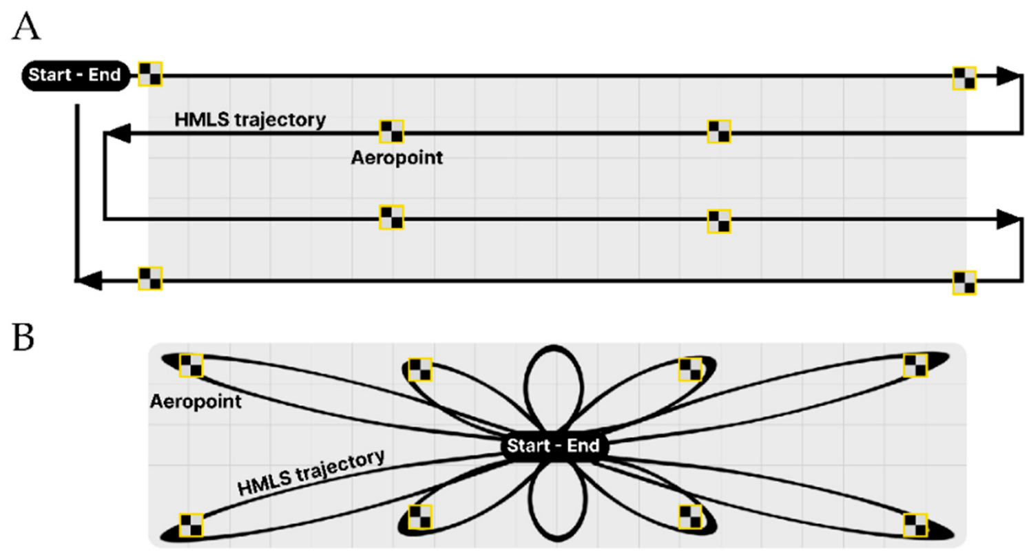
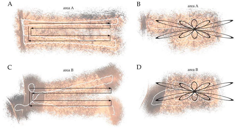
4.1. Data Collection: Zigzag and Looped Trajectory
4.2. LiDAR Metrics and Model Development
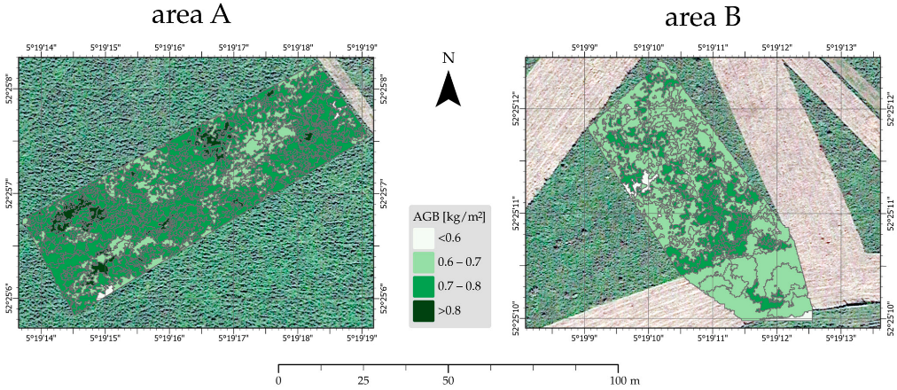
4.3. Mapping Grassland AGB
5. Discussion
5.1. Data Collection
5.2. LiDAR Metrics and Model Development
5.3. Mapping Grassland AGB
6. Concluding Remarks
Author Contributions
Funding
Data Availability Statement
Acknowledgments
Conflicts of Interest
References
- Wijesingha, J.; Moeckel, T.; Hensgen, F.; Wachendorf, M. Evaluation of 3D point cloud-based models for the prediction of grassland biomass. Int. J. Appl. Earth Obs. Geoinf. 2019, 78, 352–359. [Google Scholar] [CrossRef]
- Morais, T.G.; Teixeira, R.F.; Figueiredo, M.; Domingos, T. The use of machine learning methods to estimate aboveground biomass of grasslands: A review. Ecol. Indic. 2021, 130, 108081. [Google Scholar] [CrossRef]
- Cooper, S.D.; Roy, D.P.; Schaaf, C.B.; Paynter, I. Examination of the potential of terrestrial laser scanning and structure-from-motion photogrammetry for rapid nondestructive field measurement of grass biomass. Remote Sens. 2017, 9, 531. [Google Scholar] [CrossRef]
- Cornelissen, P.; Gresnigt, M.C.; Vermeulen, R.; Bokdam, J.; Smit, R. Transition of a Sambucus nigra L. dominated woody vegetation into grassland by a multi-species herbivore assemblage. J. Nat. Conserv. 2014, 22, 84–92. [Google Scholar] [CrossRef]
- Kuypers, H.E.; Op den Kelder, R.; Cornelissen, P. Jaarrapportage Oostvaardersplassen 2022. In Staatsbosbeheer Report; State Forestry Department of The Netherlands: Amsterdam, The Netherlands, 2023; pp. 1–39. [Google Scholar]
- Koma, Z.; Seijmonsbergen, A.C.; Kissling, W.D. Classifying wetland-related land cover types and habitats using fine-scale lidar metrics derived from country-wide Airborne Laser Scanning. Remote Sens. Ecol. Conserv. 2021, 7, 80–96. [Google Scholar] [CrossRef]
- Wang, D.; Xin, X.; Shao, Q.; Brolly, M.; Zhu, Z.; Chen, J. Modeling aboveground biomass in Hulunber grassland ecosystem by using unmanned aerial vehicle discrete lidar. Sensors 2017, 17, 180. [Google Scholar] [CrossRef] [PubMed]
- Schaefer, M.T.; Lamb, D.W. A combination of plant NDVI and LiDAR measurements improve the estimation of pasture biomass in tall fescue (Festuca arundinacea var. Fletcher). Remote Sens. 2016, 8, 109. [Google Scholar] [CrossRef]
- Xu, K.; Su, Y.; Liu, J.; Hu, T.; Jin, S.; Ma, Q.; Zhai, Q.; Wang, R.; Zhang, J.; Li, Y.; et al. Estimation of degraded grassland aboveground biomass using machine learning methods from terrestrial laser scanning data. Ecol. Indic. 2020, 108, 105747. [Google Scholar] [CrossRef]
- Bakx, T.R.; Koma, Z.; Seijmonsbergen, A.C.; Kissling, W.D. Use and categorization of light detection and ranging vegetation metrics in avian diversity and species distribution research. Divers. Distrib. 2019, 25, 1045–1059. [Google Scholar] [CrossRef]
- Jansen, V.S.; Kolden, C.A.; Greaves, H.E.; Eitel, J.U.H. Lidar provides novel insights into the effect of pixel size and grazing intensity on measures of spatial heterogeneity in a native bunchgrass ecosystem. Remote Sens. Environ. 2019, 235, 111432. [Google Scholar] [CrossRef]
- Zhang, X.; Bao, Y.; Wang, D.; Xin, X.; Ding, L.; Xu, D.; Hou, L.; Shen, J. Using UAV LiDAR to Extract Vegetation Parameters of Inner Mongolian Grassland. Remote Sens. 2021, 13, 656. [Google Scholar] [CrossRef]
- Li, A.; Dhakal, S.; Glenn, N.F.; Spaete, L.P.; Shinneman, D.J.; Pilliod, D.S.; Arklem, R.S.; McIlroy, S.K. Lidar aboveground vegetation biomass estimates in shrublands: Prediction, uncertainties and application to coarser scales. Remote Sens. 2017, 9, 903. [Google Scholar] [CrossRef]
- Ventura, D.; Napoleone, F.; Cannucci, S.; Alleaume, S.; Valentini, E.; Casoli, E.; Burrascano, S. Integrating low-altitude drone based-imagery and OBIA for mapping and manage semi natural grassland habitats. J. Environ. Manag. 2022, 321, 115723. [Google Scholar] [CrossRef] [PubMed]
- Schulze-Brüninghoff, D.; Hensgen, F.; Wachendorf, M.; Astor, T. Methods for LiDAR-based estimation of extensive grassland biomass. Comput. Electron. Agric. 2019, 156, 693–699. [Google Scholar] [CrossRef]
- Levick, S.R.; Whiteside, T.; Loewensteiner, D.A.; Rudge, M.; Bartolo, R. Leveraging TLS as a calibration and validation tool for MLS and ULS mapping of savanna structure and biomass at landscape-scales. Remote Sens. 2021, 13, 257. [Google Scholar] [CrossRef]
- Feiten en Cijfers van de Oostvaardersplassen. Available online: https://www.staatsbosbeheer.nl/Over-Staatsbosbeheer/Dossiers/oostvaardersplassen-beheer/feiten-en-cijfers (accessed on 16 September 2021).
- GeoSLAM Ltd. Zeb Revo RT User’s Manual v1.0.1; GeoSLAM Ltd.: Nottingham, UK, 2017; 80p. [Google Scholar]
- Bauwens, S.; Bartholomeus, H.; Calders, K.; Lejeune, P. Forest inventory with terrestrial LiDAR: A comparison of static and hand-held mobile laser scanning. Forests 2016, 7, 127. [Google Scholar] [CrossRef]
- Balenović, I.; Liang, X.; Jurjević, L.; Hyyppä, J.; Seletković, A.; Kukko, A. Hand-Held Personal Laser Scanning–Current Status and Perspectives for Forest Inventory Application. Croat. J. For. Eng. J. Theory Appl. For. Eng. 2021, 42, 165–183. [Google Scholar]
- Geometius. Propeller AeroPoints-Technical Specifications. Available online: https://www.geometius.nl/wp-content/uploads/2017/11/Brochures-AeroPoints-1.pdf (accessed on 10 March 2023).
- GeoSLAM Hub, Version 6.1.0; GeoSLAM Ltd.: Nottingham, UK, 2020.
- GeoSLAM Draw, Version 3.5; GeoSLAM Ltd.: Nottingham, UK, 2020.
- CloudCompareTM. 3D Point Cloud and Mesh Processing Software, Version 2.11.3. Available online: https://www.danielgm.net/cc/ (accessed on 21 November 2021).
- Soil and Environmental Chemistry Lab—Institute for Biodiversity and Ecosystem Dynamics. Available online: https://ibed.uva.nl/facilities/physical-and-chemical-lab/soil--environmental-chemistry/soil--environmental-chemistry.html (accessed on 11 February 2022).
- Esri Inc. ArcGIS Pro GIS-Software. Version 2.8.3. 2021. Available online: https://www.esri.com/en-us/arcgis/products/arcgis-pro/overview (accessed on 2 November 2021).
- Hengl, T. Finding the right pixel size. Comput. Geosci. 2006, 32, 1283–1298. [Google Scholar] [CrossRef]
- Blaschke, T.; Johansen, K.; Tiede, D. Object-Based Image Analysis for Vegetation Mapping and Monitoring. In Advances in Environmental Remote Sensing: Sensors, Algorithms, and Applications; Qihao, W., Ed.; CRC Press: Boca Raton, FL, USA, 2011; pp. 141–266. ISBN 9781138072916. [Google Scholar]
- R Core Team. R: A Language and Environment for Statistical Computing, version 4.0.02; R Foundation for Statistical Computing: Vienna, Austria, 2020. [Google Scholar]
- Breiman, L. Random forests. Mach. Learn. 2001, 45, 5–32. [Google Scholar] [CrossRef]
- Blaschke, T. Object based image analysis for remote sensing. ISPRS J. Photogramm. Remote Sens. 2010, 65, 2–16. [Google Scholar] [CrossRef]
- Trimble Germany GmbH. Trimble Documentation eCognition Developer 10.1.1 User Guide; Trimble Germany GmbH: Munich, Germany, 2022. [Google Scholar]
- Baatz, M.; Schäpe, A. Multiresolution Segmentation: An Optimization Approach for High Quality Multi-Scale Image Segmentation. In Angewandte Geographische Informations-Verarbeitung, XII; Strobl, J., Blaschke, T., Griesbner, G., Eds.; Wichmann Verlag: Karlsruhe, Germany, 2000; pp. 12–23. [Google Scholar]
- Drăguţ, L.; Tiede, D.; Levick, S. ESP: A tool to estimate scale parameter for multiresolution image segmentation of remotely sensed data. Int. J. Geogr. Inf. Sci. 2010, 24, 859–871. [Google Scholar] [CrossRef]
- Obanawa, H.; Yoshitoshi, R.; Watanabe, N.; Sakanoue, S. Portable LiDAR-based method for improvement of grass height measurement accuracy: Comparison with SfM methods. Sensors 2020, 20, 4809. [Google Scholar] [CrossRef]
- Potter, T.L. Mobile Laser Scanning in Forests: Mapping beneath the Canopy. Ph.D. Dissertation, University of Leicester, Leicester, UK, 2019. [Google Scholar]
- Haacke, P. HMLS-ALS Synergy and Accuracy for Complex Forest Stands. Master’s Thesis, University of Amsterdam, Amsterdam, The Netherlands, 2019. [Google Scholar]
- Cabo, C.; Del Pozo, S.; Rodríguez-Gonzálvez, P.; Ordóñez, C.; Gonzalez-Aguilera, D. Comparing terrestrial laser scanning (TLS) and wearable laser scanning (WLS) for individual tree modeling at plot level. Remote Sens. 2018, 10, 540. [Google Scholar] [CrossRef]
- Tamiminia, H.; Salehi, B.; Mahdianpari, M.; Beier, C.M.; Johnson, L. A Comparative Analysis of Pixel-Based and Object-Based Approaches for Forest Above-Ground Biomass Estimation Using Random Forest Model. ISPRS-Int. Arch. Photogramm. Remote Sens. Spat. Inf. Sci. 2022, 46, 191–196. [Google Scholar] [CrossRef]
- Aguirre-Gutiérrez, J.; Seijmonsbergen, A.C.; Duivenvoorden, J.F. Optimizing land cover classification accuracy for change detection, a combined pixel-based and object-based approach in a mountainous area in Mexico. Appl. Geogr. 2012, 34, 29–37. [Google Scholar] [CrossRef]
- Hellesen, T.; Matikainen, L. An object-based approach for mapping shrub and tree cover on grassland habitats by use of LiDAR and CIR orthoimages. Remote Sens. 2013, 5, 558–583. [Google Scholar] [CrossRef]
- Zlinszky, A.; Schroiff, A.; Kania, A.; Deák, B.; Mücke, W.; Vári, Á.; Szekely, B.; Pfeifer, N. Categorizing grassland vegetation with full-waveform airborne laser scanning: A feasibility study for detecting Natura 2000 habitat types. Remote Sens. 2014, 6, 8056–8087. [Google Scholar] [CrossRef]
- Bazzo, C.O.G.; Kamali, B.; Hütt, C.; Bareth, G.; Gaiser, T. A Review of Estimation Methods for Aboveground Biomass in Grasslands Using UAV. Remote Sens. 2023, 15, 639. [Google Scholar] [CrossRef]
- Kissling, W.D.; Shi, Y.; Koma, Z.; Meijer, C.; Ku, O.; Nattino, F.; Seijmonsbergen, A.C.; Grootes, M.W. Country-wide data of ecosystem structure from the third Dutch airborne laser scanning survey. Data Brief 2023, 46, 108798. [Google Scholar] [CrossRef]


| Vegetation Structure | Metric Name | Metric Description | Ecological Description |
|---|---|---|---|
| Height | Hmax | The maximum of all height returns | Vegetation height |
| Hmean | The arithmetic mean of all height returns | Mean vegetation height | |
| Hmedian | The median of all height returns | Median vegetation height | |
| 10th perc | 10th percentile of all height returns | Height at which 10% of returns is recorded | |
| 25th perc | 25th percentile of all height returns | Height at which 25% of returns is recorded | |
| 75th perc | 75th percentile of all height returns | Height at which 75% of returns is recorded | |
| 80th perc | 80th percentile of all height returns | Height at which 80% of returns is recorded | |
| 90th perc | 90th percentile of all height returns | Height at which 90% of returns is recorded | |
| 95th perc | 95th percentile of all height returns | Height at which 95% of returns is recorded | |
| Vertical variability | Hstd | Standard deviation of all height returns | Roughness of the vegetation height |
| Hvar | The variance of all height returns | Heterogeneity of the vegetation height | |
| Hcv | Coefficient of variation of all height returns | Variability of the vegetation height | |
| Hskew | The skewness of all height returns | Skewness of the vegetation height | |
| Hkurt | The kurtosis of all height returns | Vertical vegetation variability | |
| HMAD | Mean Abs. Deviation of all height returns | Spread of the vegetation height |
| A1 | A2 | A3 | A4 | A5 | A6 | A7 | A8 | A9 | A10 | A11 | A12 | A13 | A14 | A15 | A16 | |
| Area A | 0.58 | 0.73 | 0.40 | 0.56 | 0.70 | 0.59 | 0.80 | 0.66 | 0.53 | 0.69 | 0.68 | 0.68 | 0.64 | 1.00 | 0.85 | 0.83 |
| Area B | B1 | B2 | B3 | B4 | B5 | B6 | B7 | B8 | B9 | B10 | B11 | B12 | B13 | B14 | B15 | B16 |
| 0.48 | 0.46 | 0.59 | 0.98 | 0.66 | 0.54 | 0.83 | 0.42 | 0.86 | 0.63 | 1.01 | 0.66 | 0.77 | 0.70 | 0.77 | 0.96 |
| RF Model | R2 | RMSE (kg/m2) | Predictors | Ntree | Mtry |
|---|---|---|---|---|---|
| All metrics | 0.76 | 0.078 | Hmax, Hmean, Hmedian, Hstd, Hvar, 10th, 25th, 75th, 80th, 90th, 95th, Hcv, Hskew, Hkurt, HMAD | 500 | 2 |
| Four metrics, Ntree and Mtry | 0.78 | 0.075 | Hmax, Hmean, Hmedian, 75th | 9 | 4 |
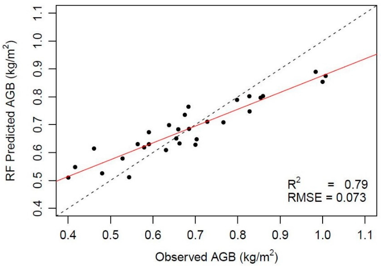
| Two metrics, Ntree and Mtry | 0.79 | 0.073 | Hmax, 75th | 25 | 2 |
Disclaimer/Publisher’s Note: The statements, opinions and data contained in all publications are solely those of the individual author(s) and contributor(s) and not of MDPI and/or the editor(s). MDPI and/or the editor(s) disclaim responsibility for any injury to people or property resulting from any ideas, methods, instructions or products referred to in the content. |
© 2023 by the authors. Licensee MDPI, Basel, Switzerland. This article is an open access article distributed under the terms and conditions of the Creative Commons Attribution (CC BY) license (https://creativecommons.org/licenses/by/4.0/).
Share and Cite
de Nobel, J.S.; Rijsdijk, K.F.; Cornelissen, P.; Seijmonsbergen, A.C. Towards Prediction and Mapping of Grassland Aboveground Biomass Using Handheld LiDAR. Remote Sens. 2023, 15, 1754. https://doi.org/10.3390/rs15071754
de Nobel JS, Rijsdijk KF, Cornelissen P, Seijmonsbergen AC. Towards Prediction and Mapping of Grassland Aboveground Biomass Using Handheld LiDAR. Remote Sensing. 2023; 15(7):1754. https://doi.org/10.3390/rs15071754
Chicago/Turabian Stylede Nobel, Jeroen S., Kenneth F. Rijsdijk, Perry Cornelissen, and Arie C. Seijmonsbergen. 2023. "Towards Prediction and Mapping of Grassland Aboveground Biomass Using Handheld LiDAR" Remote Sensing 15, no. 7: 1754. https://doi.org/10.3390/rs15071754
APA Stylede Nobel, J. S., Rijsdijk, K. F., Cornelissen, P., & Seijmonsbergen, A. C. (2023). Towards Prediction and Mapping of Grassland Aboveground Biomass Using Handheld LiDAR. Remote Sensing, 15(7), 1754. https://doi.org/10.3390/rs15071754