Article

Integrating Active and Passive Remote Sensing Data for Mapping Soil Salinity Using Machine Learning and Feature Selection Approaches in Arid Regions

by
Sayed A. Mohamed
1,
Mohamed M. Metwaly
1,
Mohamed R. Metwalli
1,
Mohamed A. E. AbdelRahman
2 and
Nasem Badreldin
3,*
1
Data Reception, Analysis, and Receiving Station Affairs Division, National Authority for Remote Sensing and Space Sciences, Cairo 11769, Egypt
2
Land Use Department, Division of Environmental Studies and Land Use, National Authority for Remote Sensing and Space Sciences (NARSS), Cairo 11769, Egypt
3
Department of Soil Science, Faculty of Agricultural and Food Science, University of Manitoba, 13 Freedman Crescent, Winnipeg, MB R3T 2N2, Canada
*
Author to whom correspondence should be addressed.
Remote Sens. 2023, 15(7), 1751; https://doi.org/10.3390/rs15071751
Submission received: 9 February 2023 / Revised: 20 March 2023 / Accepted: 22 March 2023 / Published: 24 March 2023

Abstract

:
The prevention of soil salinization and managing agricultural irrigation depend greatly on accurately estimating soil salinity. Although the long-standing laboratory method of measuring salinity composition is accurate for determining soil salinity parameters, its use is frequently constrained by the high expense and difficulty of long-term in situ measurement. Soil salinity in the northern Nile Delta of Egypt severely affects agriculture sustainability and food security in Egypt. Understanding the spatial distribution of soil salinity is a critical factor for agricultural development and management in drylands. This research aims to improve soil salinity prediction by using a combined data collection method consisting of Sentinel-1 C radar data and Sentinel-2 optical data acquired simultaneously via integrated radar and optical sensor variables. The modelling approach focuses on feature selection strategies and regression learning. Feature selection approaches that include the filter, wrapper, and embedded methods were used with 47 selected variables depending on a genetic algorithm to scrutinize whether regions of the spectrum from optical indices and SAR texture choose the optimum combinations of selected variables. The sub-setting variables resulting from each feature selection method were used to train the regression learners’ random forest (RF), linear regression (LR), backpropagation neural network (BPNN), and support vector regression (SVR). Combining the BPNN feature selection method with the RF regression learner better predicted soil salinity (RME 0.000246; sub-setting variables = 18). Integrating different remote sensing data and machine learning provides an opportunity to develop a robust prediction approach to predict soil salinity in drylands. This research evaluated the performances of various machine learning models, overcame the limitations of conventional techniques, and optimized the variable input combinations. This research can assist farmers in soil-salinization-affected areas in better managing planting procedures and enhancing the sustainability of their lands.

1. Introduction

Soil salinization is a prevalent form of land degradation, which is a global phenomenon that impacts soil productivity and health in arid and semi-arid ecosystems [1,2,3,4,5,6,7,8]; it limits the land’s suitability for cultivation or reclamation while also increasing soil dispersion and erosion [9]. Furthermore, due to the initial high water-soluble salt, sparse rainfall, high evaporation, high groundwater levels, and inadequate agricultural practices, this type of land degradation requires a dynamic soil salinity mapping approach and monitoring technique to provide spatiotemporal information that potentially improves the soil conservation management and planning [10].
Traditional soil salinization assessment methods depend on field soil sampling, which requires a huge sampling size due to the high spatial variation in soil salinity, followed by extensive laboratory analysis, which is time-consuming and labor-intensive, as well as not operational or applicable for monitoring multitemporal large-scale case studies [11,12,13].
Remote sensing technology has progressively supplanted the traditional method as a more effective way of monitoring soil salinity from the same region across regional or large scales [14,15,16]. The interaction between soil reflectance and salinity indicators is used to quantify and measure the spatiotemporal dynamics [17]; this technology has the potential to obtain accurate chemical and physical soil properties [12].
Various space-borne remote sensing data with different spatial and temporal resolutions have been utilized in soil salinity mapping, thereby resulting in the development of new techniques for qualitative research methods on soil characteristics [18], such as soil texture [19], soil bulk density [20], anion and cation exchange [21], soil organic carbon [19,22], total available nitrogen [23,24], pH [25], available potassium [26], and total phosphorus [27]. Recently, several studies succeeded in mapping and monitoring soil salinity using accessible optical remote sensing data, such as Landsat [8,28,29], SPOT [30], ASTER [31], RapidEye [30], IKONOS [32], QuickBird [33], and Sentinel 2 [34,35].
The limitation of using solely optical sensors to measure soil properties lies in its sensitivity to meteorological conditions such as clouds and dust storms, which deteriorate its radiometric quality [10]. Synthetic aperture radar (SAR) remote sensing has merits under all weathering conditions and the ability to penetrate vegetation and the soil surface to a depth of 150 cm, depending on the frequency and bandwidth (e.g., X, S, L, Ka, and P) [22]. Numerous researchers studied the possibility of utilizing SAR technology for mapping and monitoring the spatial variation in soil attributes such as texture [36], moisture [37], and salinity field [38,39,40]. SAR images’ diversity and complexity, in addition to the scarcity of publicly accessible high-resolution radar and multispectral images, limit their use in digital soil mapping [41].
Integrating SAR and optical remote sensing can enhance the satellite-based detection approach for soil surface features, thereby compensating for optical remote sensing limitations. Sentinel-1 and Sentinel-2 have reasonably high spatial and temporal resolutions to map and assess soil salinization impact at a regional scale [10]. Sentinel-2 has been used by numerous researchers in assessing soil salinity [35,42,43], and Sentinel-1 has also been used by several researchers in the soil attribute mapping research field [38,40,44]. In addition, several researchers combined sensors with varied capabilities and concluded that combining multi-source sensors can significantly increase the accuracy of the digital soil mapping field [24,45,46]. To create a spatial prediction model for mapping saline soils in the study region, we need information on the characteristics impacting the accuracy of the digital soil map output between the optical and radar data [10,47,48].
For predicting and mapping soil salinity, several statistical models from classical artificial neural networks (ANN) and deep learning (DL) were applied in the past few years [49]; now, artificial intelligence (AI) and regression models are becoming the new reliable tools in digital soil mapping. Hosseini et al. [50] indicated that numerous researchers have recently used new machine learning (ML) approaches, such as decision trees (DT), random forests (RF), and ANN, to predict some chemical and physical soil properties [51,52]. Achieng [53] employed a multilayer perceptron neural network (MLP-NN) to forecast soil salinity and used an artificial and deep neural network to model soil moisture. Analyzing big geospatial data using ML analyses has special workflows depending on data type and size; it starts by utilizing semi-automated datasets to find linear and nonlinear correlations between salinities and other input variables (e.g., salinity indices, vegetation indices, intensity indices, and terrain derivatives), to build statistical relationships for a continuous spatial soil salinity prediction [10,54]. RF [10,35,55] classification and regression trees (CART) [10], as well as boosted regression trees (BRT), are among the most common ML models that have been shown to have robust performance in soil salinity prediction [24,56].
Alamdar et al. [57] evaluated the performance of three machine learning (ML) algorithms, including random forest (RF), gradient boosting machine (GBM), and multi-layer perceptron (MLP), in detecting and monitoring saline soils using an 18-indicator dataset, including seven Landsat-8 OLI bands, vegetation, and salinity indices. The GBM method exhibited the highest performance with an R2 of 0.89 and a RMSE of 0.63, followed by the RF model with an R2 of 0.85 and a RMSE of 0.71, and the MLP model with an R2 of 0.75 and a RMSE of 0.88. The study revealed that satellite data could potentially estimate soil salinity with the appropriate method and acceptable in situ data. Another study [58] evaluated three ML models’ performances in predicting soil salinity parameters using inputs such as soil temperature, potential hydrogen, soil water content, and electrical conductivity. The study used 467 soil samples from northwest China for model training, testing, and validation. The RF and support vector machine (SVM) models performed well with the EC, soil temperature, and pH, while the extreme gradient boosting (XGB) model was better with the EC, soil water content, and soil temperature. Mzid et al. [59] used Sentinel-2 multispectral imagery to predict soil EC in salt-affected soils in central Tunisia, where they achieved the best results using several ML algorithms. Other studies [60,61] developed various ML-based models that accurately predicted the spatial distributions of soil salinity. Wang et al. [62] and Rafik et al. [63] found that integrating different optical satellite data such as Landsat 4–5, Landsat 7, Landsat 8, and Sentinel 2 had a substantial impact on the accuracy of soil salinity prediction, with an R2 and Nash–Sutcliffe model efficiency coefficient (NSE) of 0.93 and 0.86, respectively. Other studies found improvements in soil salinity prediction when integrating optical data (e.g., Landsat) with a digital elevation model (DEM) using a deep extreme learning machine (DELM), a sine cosine algorithm—Elman (SCA-Elman) [64], a DT, and a RF [65].
Recent studies [66,67,68,69] have stated that the efficiency of ML models depends not only on the accuracy of prediction, but also on the combination of input parameters and the model adopted. Currently, the prediction of soil characteristics is still rare. More importantly, soil alkalinity and salinity are often determined by the relative content of soil content [70]. However, predicting soil salinity parameters with machine learning models is crucial for guiding planting and irrigation. However, there are still few studies in this area, and there is a lack of specific evaluation and management. Interestingly, using physical parameters such as conductance, temperature, soil water content, and pH measured by sensor technology as predictive indicators could improve machine learning efficiency and reduce the cost of laboratory tests [71,72].
Several ML algorithms have been used for various applications, with optical or radar sensors as the basis. In [73], The study objective was to compare five machine learning algorithms for predicting soil salinity: the least absolute shrinkage and selection operator (LASSO), the multiple adaptive regression splines (MARS), the classification and regression trees (CART), the RF, and the stochastic gradient tree boost (SGT); This presented us with a challenge to identify the most effective factor from optical and radar data that was the impact factor for predicting soil salinity in the northern Nile Delta of Egypt area. However, there has been no advice about which ML algorithms and satellite sensor settings may be ideal for predicting soil salinity in various regions [74]. A subset of remote sensing variables were used to test the soil salinity prediction models using feature selection techniques.
Therefore, the main goal of this study is to construct a robust and flexible spatial prediction model using optical and SAR satellite data to assess and map soil salinity in the northern Nile Delta of Egypt as an example of an arid ecosystem. This goal will be achieved in two steps: (i) using feature selection techniques (e.g., filter, wrapper, and embedded) depending on statistical and ML algorithms to scrutinize whether regions of the spectrum from optical indices and SAR texture contain essential information for soil estimation to choose the optimum combinations of selected variables, and (ii) using the selected variables to train and optimize the parameters of linear regression (LR), support vector regression (SVR), RF, and the backpropagation neural network (BPNN). The performance of regression learners will be measured using descriptive statistics, such as RMSE and R2 (Adj-R2).

2. Materials and Method

2.1. Study Area Description and Field Survey

The study area is located on the northwestern side of the Nile delta. It is surrounded from the north by the Mediterranean Sea, from the east by the Rashid branch, from the west by the governorates of Alexandria and Matrouh, and from the south by the southern part of El-Beheira Governorate, see Figure 1. The study area covers an area of 3941 km2 (394,096.5 hectares (ha)). Agricultural fields represent an area of 3311.16 km2 (331,116.12 ha), and elevation ranges from 1 to 69 m above sea level; it is located under arid conditions, which are characterized by mean minimum and maximum annual temperatures, which are 12.6 °C and 26.2 °C, respectively, which indicates a thermic temperature regime. The annual precipitation is 83.7 mm, showing torric moisture regime [75], and the mean annual relative humidity is 57% [76].
The Rosetta Branch provides a constant water source for the city’s vast farmed lands. It has a stable climate and abundant fishing opportunities along the coast on the Rosetta Branch and at Edko Lake. It is well-known for its diverse agricultural commodity productions, including cotton, rice, wheat, maize, and potatoes. It leads the governorates in food production (e.g., fruits and vegetables) and the export of citrus, potatoes, tomatoes, artichokes, melons, string beans, and pepper.
According to Afifi and Darwish [77], the soil parent material of the study area is mainly clayey. The main soil orders are Entisols and Aridisols, these two different soil orders illustrate the distribution of different subgroups of soil: Vertic Torrifluvents, Typic Quartizpsamments, Typic Torripsamments, Typic Torrifluvents, Typic Torriorthents, Typic Haplocalsids, Typic Haplosalids, Typic Aquisalids, and Typic Calcigypsids.
A total of 100 soil sampling locations were collected from 68 agricultural fields (flood-irrigated farms) in the research area during a field survey conducted from February to March 2018. At each sampling location, a five-point sampling method was conducted to collect five soil samples using an auger at each sampling site (30 m × 30 m) (collected at the four corners and the center of each plot), which were then mixed them on-site to create a representative composite sample (topsoil at 0–30 cm and subsoil at 30–60 cm) while recording their geographic locations with a portable GPS (UniSrong G120); with this sampling approach, we collected 1000 soil samples, which were air-dried, pulverized, and sieved through a 2 mm sieve to collect soil particles for further lab analysis. The pipette method determined the fractions of soil particles (clay, sand, and silt). In a 1:5 soil water diluted extract procedure, the multi-parameter method determined the soil electrical conductivity (ECe) (WTW multi-3430). According to the international standards of soil salinity measurements, the soil sample solutions were extracted using a multiparameter measuring device (Multi 3420 Set B, WTW GmbH, Weilheim, Germany), which was equipped with a composite electrode (TetraCon 925) at a normal laboratory temperature of 25 °C to measure electrical conductivity (EC) (1:5 soil–water extraction solution). The measured ECe was used to calculate the soil salinity [78]. The soil salinity in this research was categorized as shown in Table 1. Among the collected soil samples, the general descriptive statistics of soil salinity (dS/m) in the case study were a minimum of 0.4, a maximum of 16, a mean of 6.2, a standard deviation of 4.3, and a coefficient of variation (CV) of 69.3%.

2.2. Remote Sensing Data Acquisition and Pre-Processing

In this research, SAR (Sentinel-1) and optical (Sentinel-2) variables were chosen because of their effectiveness in ML modeling performance to predict soil salinity in drylands such as the Northern Nile Delta of Egypt.
To incapacitate weather limitations that affect the radiometric quality from Sentinel-2 (optical remote sensing data), SAR data were integrated into the modeling process. The C band sensor on the Sentinel-1 (A, B) satellite platform operates at 5.405 GHz and has an incidence angle of 20 to 45 degrees. Sentinel-2 (A, B) was launched in April 2016 and continues to collect data regularly [80,81] and at an altitude of 693 kilometers (km). This platform travels in a sun-synchronous orbit toward the pole. The Copernicus Open Access Hub was used to obtain SAR single look complex (SLC) products, and pre-processing was done with the SNAP (Sentinel Application Platform) software. Calibration, multi-looking, filtering, and geometry correction were among the pre-processing procedures, along with layover and shadowing analysis. As a result, a series of geocoded intensity images were created, which were then transformed into backscattering coefficients ranging from 0 to 1. (Sigma Nought δ0). The software converts radar reflectivity into a radar cross-section with an area normalization aligned with the ground range plane. The final products are encoded as 16-bit integers (signed for SLC, unsigned for GRD) [82]. As a result, the Sentinel-1 images were transformed into Sigma Nought (δ0). Also, gray-level co-occurrence matrix (GLCM) factors included contrast, energy, dissimilarity, homogeneity, angular second moment, and correlation [83].
Sentinel-2 multi-spectral instrument (MSI) level-1C (L1C) images were acquired on 14 June 2019, which had reflectance data from the top of the atmosphere (TOA). The Sen2Cor technique was used to transform L1C data into level-1A (L1A) data; TOA reflectance was transformed to the bottom of the atmosphere or Earth’s surface reflectance following atmospheric adjustment. In this investigation, four (4) bands (b) with a resolution of 10 m (b2, b3, b4 and b8) and six (6) bands with 20 m spatial resolutions (b5, b6, b7, b8A, b11, and b12) were used from Sentinel-2. The selected bands were stacked and trimmed using SNAP software to create a subset of the research region. An ML approach was used to better comprehend the sensitivity of SAR and optical bands to the soil salinity estimation [84]. Sentinel-1 efficiency of Sigma Nought (δ0) feature extraction of level 1 images and Sentinel-2 indices were employed to predict and determine the areas under soil salinity using a feature selection and prediction method. These raster factors (variables) are shown in Table 2. Fifteen spectral indices—normalized difference vegetation index (NDVI), green normalized difference vegetation index (GNDVI), difference vegetation index (DVI), weighted difference vegetation index (WDVI), transformed normalized difference vegetation index (TNDVI), soil-adjusted vegetation index (SAVI), modified soil-adjusted vegetation index (MSAVI), second modified soil-adjusted vegetation index (MSAVI2), modified chlorophyll absorption ratio index (MCARI), infrared percentage vegetation index (IPVI), normalized difference water index (NDWI), modified normalized difference water index (MNDWI), color index (CI), brightness index (BI)—were calculated using the pre-processing Sentinel-2 bands and SNAP software 9.0.0.
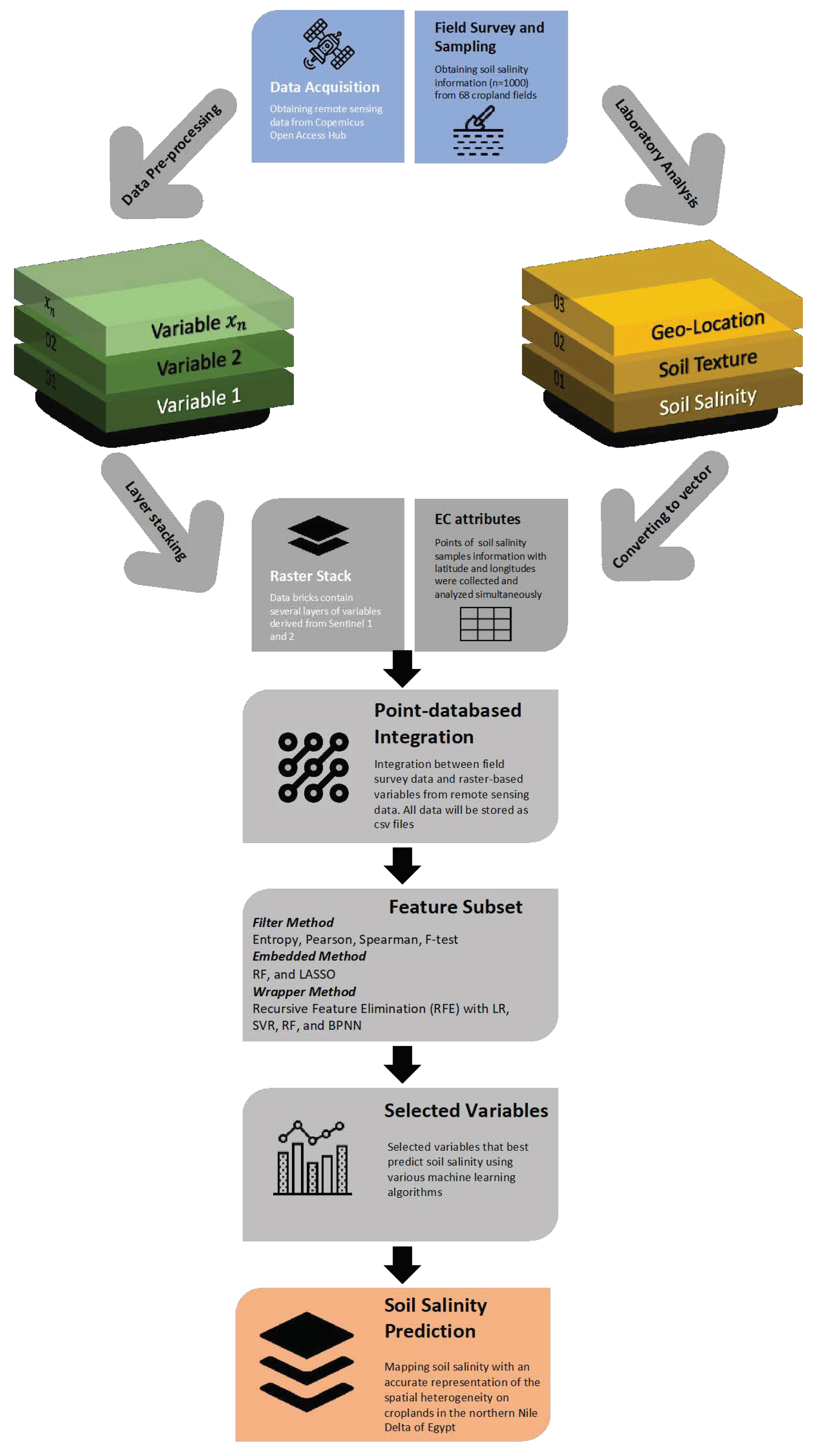
The feature selection (FS) and ML algorithms were analyzed using MATLAB R2021b software. We used MATLAB Bayesian optimizer with 50 iterations and 3K-fold cross-validation to fine-tune the different ML models’ hyperparameters (SVR, RF, BPNN) and avoid overfitting, see Figure 2.

2.3. Feature Selection Techniques

The feature selection (FS) approach was used as a data reduction technique in the pre-processing data stage to locate precise data models by deleting irrelevant and redundant characteristics from a dataset to improve ML algorithms’ performance. It is divided into several methods depending on several criteria, which include (i) the assessment mechanism of the combined features and (ii) the technique that evaluates features at each learning algorithm.
The pros and cons of feature selection strategies will be examined in this analysis stage. The prime task of these various approaches is to select a subset (s) of the best-performing inputs (features/variables).

2.4. Filter Methods

This approach is based solely on the data’s intrinsic qualities and computes a significant value between one independent variable and the dependent variable. The independent and dependent variables are used to explain the statistical coefficients. Both variables are linearly dependent; their correlation coefficient should be close to one, and the correlation coefficient is 0 if the variables are uncorrelated [84]. Only positive values are included when the Pearson coefficient is employed as a filter mechanism, as shown in Equation (1):
r   = i = 1 n cov   x i ,   y i i = 1 n σ x i σ y i
where x i and   y i are the ith observations of independent and dependent variables respectively; cov corresponds to covariance, and σ indicates the standard deviation of x and y.
Using a monotonic function, the Spearman coefficient quantifies the association between two variables [85]. A monotonic function is either wholly growing or entirely declining. It is comparable to the Pearson coefficient; only it works with data ranks rather than raw data. Equation (2) defines the Spearman correlation rank:
= 1 6 i = 1 n d 2 n n 2 1
where d i is the difference between ranks for each x i ,   y i data pair, and n is the number of data pairs.
Entropy-based information gain: discretizes the independent variable, then computes the entropy between x and the continuous y variable using Equation (3) [86]:
InfoGain = H y + H x H y , x
where H(x) and H(y) correspond to Shannon’s Entropy for x and y variables, and H y ,   x   is a joint Shannon’s Entropy for a variable y with a condition to x.
F-tests univariate feature ranking algorithm independently examines each predictor’s value alone using an f-test to determine its importance. Each f-test compares the choice hypothesis and states that the response values are grouped by estimated values (variable) taken from populations with the same mean, see Figure 3. The negative logs of the p-values are used to calculate the scores [87].

2.5. Wrapper Methods

The main function of this stage is to evaluate the relative utility of each distinct subset of features using prediction performance assessments of a given ML methodology (e.g., forward selection or backward elimination). The recursive feature elimination (RFE) is one of the wrapping techniques, which uses an ML algorithm and sequential search to choose a subset of characteristics to best to predict response values. It constructs models repeatedly, removing one unnecessary feature at a time until the predictor performance decreases the least, which builds best-performing models using left features until all variables have been studied. During the analysis, the selected features were frequently ranked using cross-validation, which limits overfitting by defining a dataset to “test” the model during the training phase. To compute the criterion for each candidate feature subset, a performance metric such as root mean squared error (RMSE) was utilized to evaluate the feature subset selection performance [88]. This study employed four ML regression algorithms, namely: LR, SVR, RF, and BPNN. LR fits a linear equation to the observed data to establish the relationship between dependent and independent variables using the least squares approach. SVR utilizes kernel functions to describe complex nonlinear interactions. RF employs an ensemble method to integrate multiple DTs and improve prediction performance, while BPNN mimics signal transmission in human brains to achieve high prediction accuracy for complex problems with both large and small samples.
Selected variables used different ML algorithms, including RFE in this study and RMSE for regression performance evaluation, which are shown in Table 3.

2.6. Embedded Methods

This method incorporates variable selection as part of the learning process [89], which has the benefit of being reasonably quick, because the selection process is integrated into the model fitting process, and no external feature selection tool is required. In addition, this stage provides an immediate link between picking characteristics and performance measures that the model tries to optimize, such as the root mean squared error (RMSE) [90]. RF [91] and least absolute shrinkage and selection operator (LASSO) were employed as embedded approaches [92], see Table 4.

3. Results

3.1. Modeling Assessment

The feature selection methods that chose a subset of variables were assessed, which facilitated the soil salinity prediction models evaluation that was based on the selected variables. The regression learners’ results after training with selected (subsets) variables were chosen using different feature selection methods. Descriptive statistics were used to estimate the performance of the regression learners using parameters such as the root mean square error (RMSE), the coefficient of determination (R2), and the coefficient of determination (adj-R2). The underlined values corresponded to the best two learners and the tested feature selection method. As is shown in Figure 4, these statistical metrics were commissioned to measure the prediction accuracy of the regression learners. A total of 47 variables were used to train the regression learners, and 456 examples were used in the modeling assessment. The best two learners obtained the highlighted values and the feature selection procedure. The Pearson, Spearman, and f-test filter techniques chose 21 variables, while the entropy coefficients selected 25 variables.

3.2. Feature Selection Approaches for Digital Soil Salinity Mapping

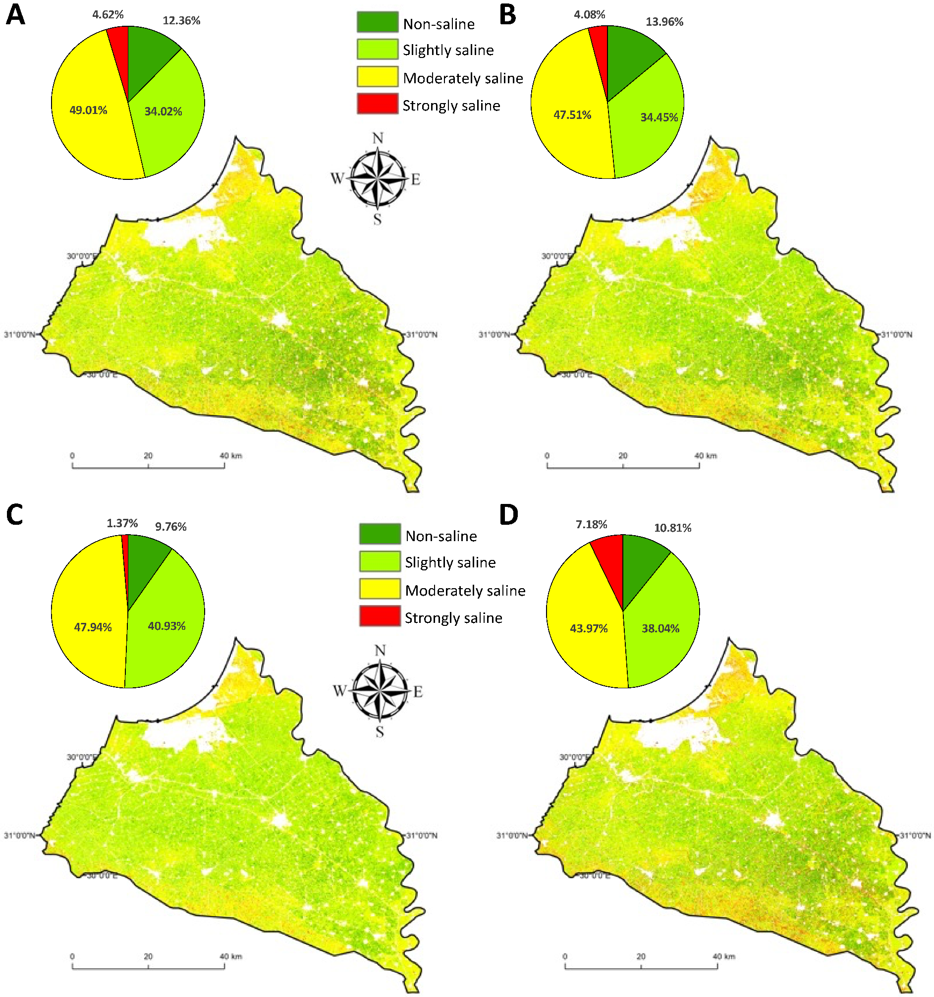
In the filter method, February’s study dates were chosen to avoid rice cultivation, as rice is grown in the area by immersion. Four associated methods were included for extracting various soil salinity ranges (classes) [93,94]. The first method (entropy method with a RF learner) was the least mixing between saline lands, urban areas, and water bodies. In the second method (Spearman method with a RF learner), there was some confusion with some spots in urban and water bodies, which makes this method the most integrating for water bodies with saline land. Similarly, the third method (Pearson method with a RF learner) was similar to the first method in avoiding urban areas. In contrast, the fourth method (f-test method with a RF learner) was comparable to the second method in merging some urban areas with the lands affected by salt (see Figure 5).
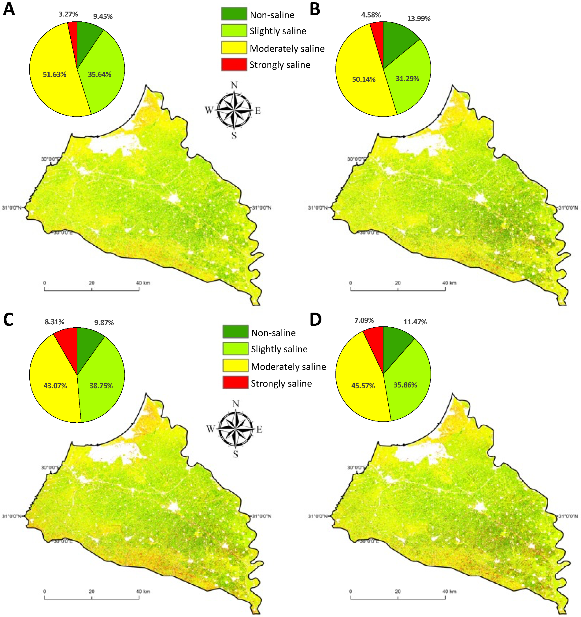
In the wrapper method, four methods successfully extracted the soil salinity ranges in the case study. The first method (BPNN with a RF learner) minimized mixing between saline lands, urban areas, and water bodies. In the second method (LM method with a RF learner), there was some ambiguity with some urban areas and water bodies. It is noted that this method was the most integrating for water bodies with saline soils, which was identical to the third method (RF method with a RF learner) in the northern part of the area. The fourth method (SVR method with a RF learner) performed a prediction that was similar to the third method (the south part of the study area) in merging some urban areas with the salinity-affected soil (see Figure 6).
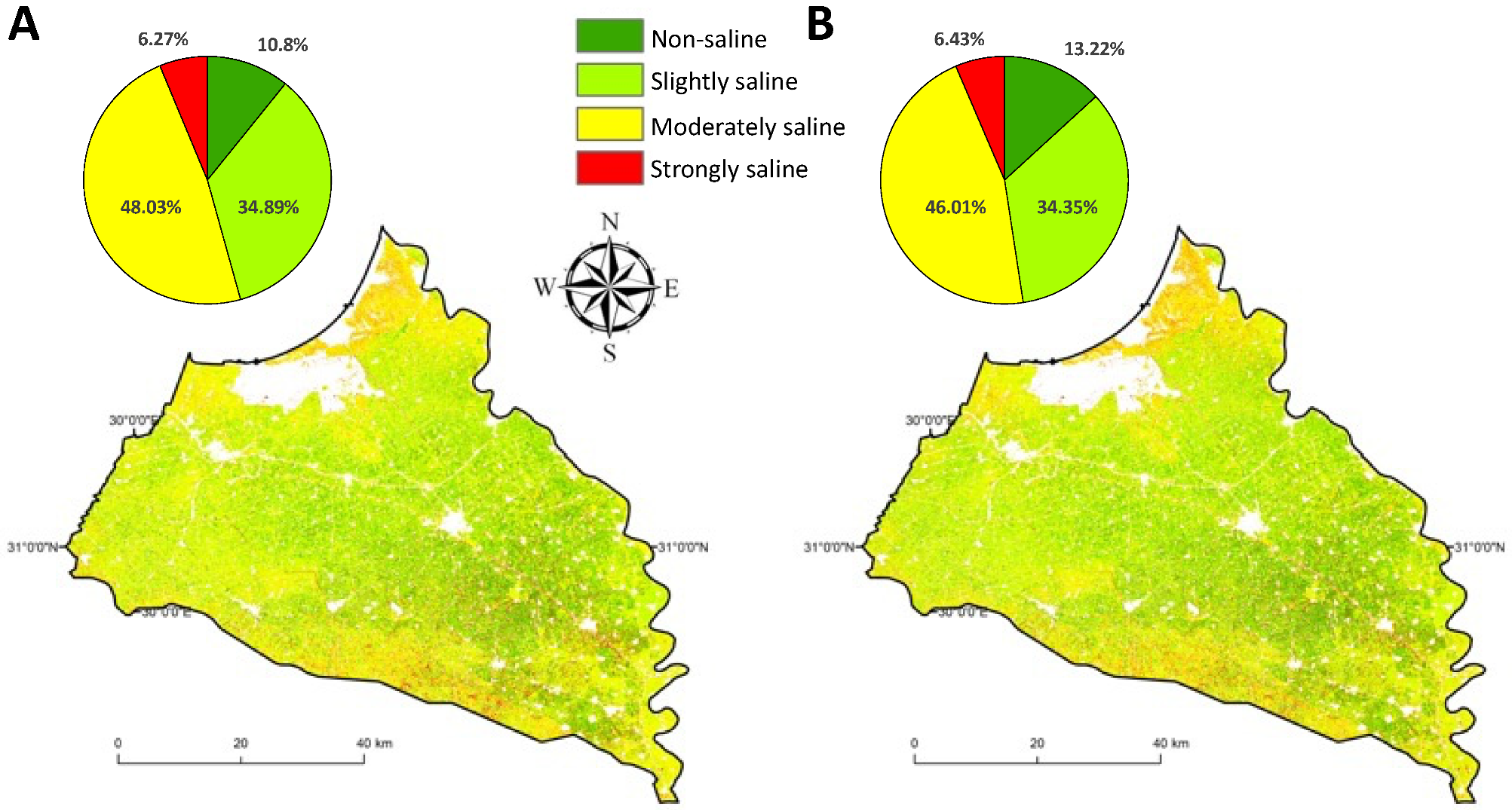
The embedded method was unblemished compared with the previously mentioned two methods, which were analogous to the extent of congruence in the outputs, but what was very clear was the superiority of the first method in the small percentage of overlap between urban areas and water bodies with saline lands. As is shown in Figure 7, the results show the extent of the spread of saline lands in the study area. They, thus, indicate the importance of finding an optimal solution to track saline lands and check the extent of the increase and decrease in areas to build an optimal strategy to solve the salinity problem by avoiding the processes of its formation and, thus, limiting it and working on choosing appropriate management methods to work on soil conservation.
The optimal method showed a superior ability to reach the saline lands instantly, thereby overcoming the problem of vegetation cover, as well as scattered and dense buildings. Also, the bare lands in the northern and southern regions helped reach the saline lands with high accuracy to identify the spectrum characteristics with the fallow areas easily.

4. Discussion

In this research, the analysis showed that the best-performing algorithms that predict soil salinity using the feature selection approach were the RF (regression learner) with BPNN, entropy, f-Test, lasso, LR, Pearson, RF, Spearman, and SVR. The lowest performance was the LR and BPNN; these comparisons were based on the statistical assessment of the RMSE, R2, and R2-adj (see Figure 4). The ML algorithms’ robustness resulted from the importance of the variables from Sentinel 1 and Sentinel 2. The feature selection approach discovered the variables that significantly impacted detecting soil salinity in the case study. They were six (6) bands from Sentinel-2 (band3, band4, band5, band6, band7, and band12), six (6) spectral indices (SAVI, MSAVI, MNDWI, MCARI, GNDVI, and DVI), and six (6) SAR bands and derivatives (VV, Mean_VV, Contrast_VH, Dissimilarity_VH, Mean_VH, and Standard_Deviation_VH). Therefore, as was consistent with what has been listed from the results, the areas of the best method (BPNN method with a RF learner) used according to the statistical analysis and land inventory in the field were as follows: 3.27% for Strongly saline > 8 dS/m and 51.63% of the total area for Moderately saline 4–8 dS/m.
The chosen model was, according to the most accurate spatial distribution of the areas affected by salinity, capable of differentiating between the results and problems resulting from all the models proposed in the previous studies in terms of the inability to differentiate between saline lands and urban areas, as well as overlap with bodies of water and wetlands. This selection was built according to the statistical investigations of the results, and, accordingly, the investigations were built for the field distribution of saline lands. On this basis, the comparison between the methods is clear, as is shown in Figure 4.
The salinity-affected soils were impeding the growth of most crops due to the high percentage of dissolved salts. These soils are considered productive croplands; however, the drought impacts and other abiotic stressors limit land productivity and soil health. In this research, the salt-affected soils were widely spread in the northern regions of the study area. The total areas of each method are shown in Figure 5, Figure 6 and Figure 7, which depend entirely on surface irrigation.
A further finding from the soil salinity classification mapping approach is that most severely and excessively salinized soils were distributed in the northern region near the lake. As a result of severe tidal influence, wind erosion, marine sedimentation, and supratidal environment in the late Quaternary, it was suggested that the high saline soils and sabkhas in this region were developed owing to the flattening of Pleistocene sand dunes. Shamal winds (northerly winds) eroded inland dunes down to the groundwater table level, while interdune voids simultaneously filled up during sea incursion to result in carbonate sedimentation. Most of the non-saline soils were found in the southern inland region.
Irrigation water management is the foremost factor in agricultural intensification and horizontal expansion, which constitutes an essential pillar in agricultural development in Egypt. The results showed that the distribution of salt-affected soils was highly dependent on environmental factors such as climate, geology, geochemistry, and hydrological conditions. The composition of the different types of salt-affected lands in the irrigated areas is directly related to the concentration of chloride, sulfate, and bicarbonate that prevail. The seawater has an additional impact on the nearby soils, and salty lakes accelerate the salinity of the soil solution. Also, magnesium chloride and sulfate salts are the main salinity sources in the Edko Lake.
Soil degradation processes in the study area are affected by several factors such as soil depth, exposure time, regularity of impacts, and groundwater fluctuation, and, usually, these soils are rich in gypsum veins that arise under conditions of deep groundwater, while the alkaline type forms in areas that suffer from high groundwater levels. The main reason for the emergence of salinity in that area is the predominance of sodium chloride salts, and irrigation with saline water with a salinity of 2500 ppm significantly drains the water. Alkaline soils in the study area are characterized by destructive natural properties such as poor ventilation, permeability, and leaching, which are directly related to the dominance of sodium cations on the exchange bench and the presence of magnesium silicate precipitated during the formation of alkaline soils. The soils rich in gypsum veins are characterized by low water permeability due to deaf layers under the layers rich in gypsum veins at different depths. Additionally, when these soils are exposed to enough soil moisture, these layers are dismantled, which turn into deaf layers by drought. The crop rotation system in the study region where salinity-affected soils are includes rice/cotton in the summer and wheat/alfalfa in the winter. All these crops have a degree of salinity tolerance to some extent. The sugar beet crop is also cultivated in that area, and it is a salinity-resistant crop that feeds the sugar factory in the northern Delta region.
The used dataset contained relatively higher information dimensions, including vegetation type and vitality, surface reflectance, surface texture (different scales), terrain variables that indirectly represent hydrological changes, parent materials, and so on. Furthermore, the results also show that the selected inputs were obviously adequate and useful information from the complex variable datasets in this study. In areas covered by vegetation, several studies have shown that vegetation vitality (which can be indirectly reflected by the vegetation index) can mitigate the extent to which soil is affected by salinization in areas with high proportions of bare soil. Peng et al. [95] proved that soil reflectance increased with increased electrical conductivity in the coastal to SWIR1 band. This was the basis for constructing a soil salinity index on bare land. Therefore, the performances of selected parameters were outstanding in the study area.

5. Conclusions

Soil salinity poses a major threat to land resources in the region, but some methods work to mitigate the effects of this problem or reverse it completely. To this end, it is necessary to scientifically diagnose the problem to develop economically viable measures to mitigate salinity. In the absence of sufficient information, salinity mitigation measures cannot be applied. Accordingly, this project is related to diagnosing salinity using traditional and modern methods (remote sensing) using spectral analysis procedures for saline lands in the northwest Egypt Delta.
Soil salinity on the northern coast of the Nile Delta of Egypt is considered an essential challenge facing decision makers in developing effective agriculture sustainability and soil conservation policies. Hence, using advanced remote sensing technology to map soil salinity with the highest accuracy and spatial resolution is paramount in Egyptian food security and rural development.
ML and remote sensing data provide a unique opportunity to develop a robust prediction approach. The selected subset of variables by RF and base learners, such as LR, SVR, RF and BPNN, which were assessed using RMSE for modeling performance, were highly efficient in soil salinity prediction. Clayey soils were the primary component in abundance in the study area due to the Nile Delta formation; also, the study found that the amount of silt had decreased in the north of the Edko Lake, which encouraged the soil salinity increase due to the Mediterranean Sea and saltwater intrusion. Thus, all of this resulted in forming the area of lands affected by salt adjacent to the coastline along the north of the study area. Using the proposed methodology, these lands have become easy to track and predict for their salinity hazard.
As a result of this research’s findings, seven recommendations were proposed 1—Reclamation of the pristine lands affected by salts with high ground and saline water levels, such as the lands of the bottom of Lake Edko; 2—Reclamation of saline lands with low productivity or virgin land with a low groundwater level, such as lands parallel to the coastline in the study area; 3—Reclamation of waterlogged lands in the north and east of the area around Lake Edko; 4—Use chemical enhancers such as (a) soluble calcium salts such as gypsum and calcium chloride, (b) acidic substances such as sulfuric acid, iron sulphate, aluminum sulphate, lime, sulphur, pyrite, and (c) calcium salts with a low solubility product (limestone); 5—Improving the lands that suffer from secondary salinity resulting from irrigation with water of low validity; 6—Cultivating crops that improve sod lands, such as rice, sugar beet, and pasture plants; 7—Maintaining and preserving productive agricultural lands from the emergence of secondary problems of salinity, waterlogging, and the maintenance of covered drainage networks.
Given the aggravation of the problem of alkalinity associated with the salinity of the land, it is recommended to add soil conditioners such as agricultural gypsum (at a rate of 50% of gypsum needs), lime, and municipal fertilizer at a rate of 20 m3/feddan (1 feddan = 4200 m2), in addition to mixing gypsum and lime separately with municipal fertilizer. It is also recommended to irrigate with fresh water and mixed water. It is also recommended to periodically analyze other soil properties such as cation exchange capacity (CEC), pH, nitrogen, and phosphorus. It is recommended with these treatments to grow rice and wheat crops under highly alkaline soil conditions.
The study succeeded in drawing a map of soil characteristics and salinity to use soil resources sustainably, as well as extrapolating the results and publishing the salinity map, which will contribute to linking land uses with the spread of soil salinity. Also, future research avenues may entail expanding the proposed approach to encompass other regions impacted by soil salinization and examining the effect of diverse crop types on soil salinity levels. Furthermore, additional research could investigate the influence of climate change on soil salinity and strategies to manage these changes in agricultural environments. There is also a need to develop a cost-effective, user-friendly tool that incorporates this approach to facilitate farmers in predicting soil salinity levels in their fields and implementing suitable management techniques. As for policy formulation, governmental bodies could allocate resources toward advancing and implementing remote sensing technologies and ML models for soil salinity prediction in agricultural areas. Incentives could be offered to farmers who adopt sustainable management practices to mitigate soil salinity levels. Governments could also promote education and awareness programs to educate farmers about soil salinity management strategies and the significance of avoiding soil salinization. By adopting these measures, policymakers can help enhance food security and agricultural sustainability in regions impacted by soil salinity, such as Egypt.

Author Contributions

Conceptualization, S.A.M., M.M.M., M.R.M., M.A.E.A. and N.B.; methodology, S.A.M., M.M.M., M.R.M. and M.A.E.A.; software, S.A.M., M.M.M. and M.R.M.; validation, S.A.M., M.M.M., M.R.M., M.A.E.A. and N.B.; formal analysis, S.A.M., M.M.M., M.R.M., M.A.E.A. and N.B.; investigation, S.A.M., M.M.M., M.R.M. and M.A.E.A.; resources, S.A.M., M.M.M., M.R.M. and M.A.E.A.; data curation, S.A.M., M.M.M., M.R.M., M.A.E.A. and N.B.; writing—original draft preparation, S.A.M., M.M.M., M.R.M., M.A.E.A. and N.B.; writing—review and editing, S.A.M., M.M.M., M.R.M., M.A.E.A. and N.B.; visualization, S.A.M., M.M.M., M.R.M., M.A.E.A. and N.B.; supervision, S.A.M., M.M.M., M.R.M., M.A.E.A. and N.B.; project administration, S.A.M., M.M.M., M.R.M., M.A.E.A. and N.B.; funding acquisition, S.A.M., M.M.M., M.R.M., M.A.E.A. and N.B.; All authors have read and agreed to the published version of the manuscript.

Funding

This research received no external funding.

Acknowledgments

We thank the academic editor and reviewers for their constructive comments to improve the manuscript’s quality.

Conflicts of Interest

The authors declare no conflict of interest.

References

  1. AbdelRahman, M.A.E.; Metwaly, M.M.; Afifi, A.A.; D’Antonio, P.; Scopa, A. Assessment of Soil Fertility Status under Soil Degradation Rate Using Geomatics in West Nile Delta. Land 2022, 11, 1256. [Google Scholar] [CrossRef]
  2. AbdelRahman, M.A.E.; Engel, B.; Eid, M.S.M.; Aboelsoud, H.M. A new index to assess soil sustainability based on temporal changes of soil measurements using geomatics—An example from El-Sharkia, Egypt. All Earth 2022, 34, 147–166. [Google Scholar] [CrossRef]
  3. AbdelRahman, M.A.E.; Farg, E.; Saleh, A.M.; Sayed, M.; Abutaleb, K.; Arafat, S.M.; Elsharkawy, M.M. Mapping of soils and land-related environmental attributes in modern agriculture systems using geomatics. Sustain. Water Resour. Manag. 2022, 8, 116. [Google Scholar] [CrossRef]
  4. Aboelsoud, H.M.; AbdelRahman, M.A.E.; Kheir, A.M.S.; Eid, M.S.M.; Ammar, K.A.; Khalifa, T.H.; Scopa, A. Quantitative Estimation of Saline-Soil Amelioration Using Remote-Sensing Indices in Arid Land for Better Management. Land 2022, 11, 1041. [Google Scholar] [CrossRef]
  5. AbdelRahman, M.A.E.; Afifi, A.A.; D’Antonio, P.; Gabr, S.S.; Scopa, A. Detecting and Mapping Salt-Affected Soil with Arid Integrated Indices in Feature Space Using Multi-Temporal Landsat Imagery. Remote Sens. 2022, 14, 2599. [Google Scholar] [CrossRef]
  6. Ibrahim, M. Modeling Soil Salinity and Mapping Using Spectral Remote Sensing Data in the Arid and Semi-arid Region. Int. J. Remote Sens. Appl. 2016, 6, 76. [Google Scholar] [CrossRef]
  7. Mohamed, N.N. Management of salt-affected soils in the Nile Delta. In The Nile Delta; Negm, A., Ed.; The Handbook of Environmental Chemistry; Springer: Cham, Switzerland, 2016; Volume 55, pp. 265–295. [Google Scholar] [CrossRef]
  8. Hammam, A.; Mohamed, E. Mapping soil salinity in the East Nile Delta using several methodological approaches of salinity assessment. Egypt J. Remote Sens. Space Sci. 2020, 23, 125–131. [Google Scholar] [CrossRef]
  9. Alqasemi, A.S.; Ibrahim, M.; Al-Quraishi, A.M.F.; Saibi, H.; Al-Fugara, A.; Kaplan, G. Detection and modeling of soil salinity variations in arid lands using remote sensing data. Open Geosci. 2021, 13, 443–453. [Google Scholar] [CrossRef]
  10. Ma, G.; Ding, J.; Han, L.; Zhang, Z.; Ran, S. Digital mapping of soil salinization based on Sentinel-1 and Sentinel-2 data combined with machine learning algorithms. Reg. Sustain. 2021, 2, 177–188. [Google Scholar] [CrossRef]
  11. Mulder, V.; de Bruin, S.; Schaepman, M.; Mayr, T. The use of remote sensing in soil and terrain mapping—A review. Geoderma 2011, 162, 1–19. [Google Scholar] [CrossRef]
  12. Allbed, A.; Kumar, L.; Aldakheel, Y.Y. Assessing soil salinity using soil salinity and vegetation indices derived from IKONOS high-spatial resolution imageries: Applications in a date palm dominated region. Geoderma 2014, 230–231, 1–8. [Google Scholar] [CrossRef]
  13. Nguyen, T.G.; Tran, N.A.; Vu, P.L.; Nguyen, Q.-H.; Nguyen, H.D.; Bui, Q.-T. Salinity intrusion prediction using remote sensing and machine learning in data-limited regions: A case study in Vietnam’s Mekong Delta. Geoderma Reg. 2021, 27, e00424. [Google Scholar] [CrossRef]
  14. Elnaggar, A.A.; Noller, J.S. Application of Remote-sensing Data and Decision-Tree Analysis to Mapping Salt-Affected Soils over Large Areas. Remote Sens. 2009, 2, 151–165. [Google Scholar] [CrossRef] [Green Version]
  15. Davis, E.; Wang, C.; Dow, K. Comparing Sentinel-2 MSI and Landsat 8 OLI in soil salinity detection: A case study of agricultural lands in coastal North Carolina. Int. J. Remote Sens. 2019, 40, 6134–6153. [Google Scholar] [CrossRef]
  16. Delavar, M.A.; Naderi, A.; Ghorbani, Y.; Mehrpouyan, A.; Bakhshi, A. Soil salinity mapping by remote sensing south of Urmia Lake, Iran. Geoderma Reg. 2020, 22, e00317. [Google Scholar] [CrossRef]
  17. Erkin, N.; Zhu, L.; Gu, H.; Tusiyiti, A. Method for predicting soil salinity concentrations in croplands based on machine learning and remote sensing techniques. J. Appl. Remote Sens. 2019, 13, 034520. [Google Scholar] [CrossRef]
  18. Zheng, Z.; Zhang, F.; Ma, F.; Chai, X.; Zhu, Z.; Shi, J.; Zhang, S. Spatiotemporal changes in soil salinity in a drip-irrigated field. Geoderma 2009, 149, 243–248. [Google Scholar] [CrossRef]
  19. Gholizadeh, A.; Žižala, D.; Saberioon, M.; Borůvka, L. Soil organic carbon and texture retrieving and mapping using proximal, airborne and Sentinel-2 spectral imaging. Remote Sens. Environ. 2018, 218, 89–103. [Google Scholar] [CrossRef]
  20. Hengl, T.; De Jesus, J.M.; Heuvelink, G.B.M.; Gonzalez, M.R.; Kilibarda, M.; Blagotić, A.; Shangguan, W.; Wright, M.N.; Geng, X.; Bauer-Marschallinger, B.; et al. SoilGrids250m: Global gridded soil information based on machine learning. PLoS ONE 2017, 12, e0169748. [Google Scholar] [CrossRef] [Green Version]
  21. Ivushkin, K.; Bartholomeus, H.; Bregt, A.K.; Pulatov, A.; Kempen, B.; de Sousa, L. Global mapping of soil salinity change. Remote Sens. Environ. 2019, 231, 111260. [Google Scholar] [CrossRef]
  22. Zhang, Z.; Ding, J.; Zhu, C.; Wang, J.; Ma, G.; Ge, X.; Li, Z.; Han, L. Strategies for the efficient estimation of soil organic matter in salt-affected soils through Vis-NIR spectroscopy: Optimal band combination algorithm and spectral degradation. Geoderma 2020, 382, 114729. [Google Scholar] [CrossRef]
  23. Kalambukattu, J.G.; Kumar, S.; Raj, R.A. Digital soil mapping in a Himalayan watershed using remote sensing and terrain parameters employing artificial neural network model. Environ. Earth Sci. 2018, 77, 203. [Google Scholar] [CrossRef]
  24. Zhou, T.; Geng, Y.; Chen, J.; Pan, J.; Haase, D.; Lausch, A. High-resolution digital mapping of soil organic carbon and soil total nitrogen using DEM derivatives, Sentinel-1 and Sentinel-2 data based on machine learning algorithms. Sci. Total Environ. 2020, 729, 138244. [Google Scholar] [CrossRef]
  25. Roelofsen, H.D.; van Bodegom, P.M.; Kooistra, L.; van Amerongen, J.J.; Witte, J.-P.M. An evaluation of remote sensing derived soil pH and average spring groundwater table for ecological assessments. Int. J. Appl. Earth Obs. Geoinform. 2015, 43, 149–159. [Google Scholar] [CrossRef]
  26. Dong, W.; Wu, T.; Luo, J.; Sun, Y.; Xia, L. Land parcel-based digital soil mapping of soil nutrient properties in an alluvial-diluvia plain agricultural area in China. Geoderma 2019, 340, 234–248. [Google Scholar] [CrossRef]
  27. Shen, Q.; Wang, Y.; Wang, X.; Liu, X.; Zhang, X.; Zhang, S. Comparing interpolation methods to predict soil total phosphorus in the Mollisol area of Northeast China. Catena 2018, 174, 59–72. [Google Scholar] [CrossRef]
  28. Elhag, M. Evaluation of Different Soil Salinity Mapping Using Remote Sensing Techniques in Arid Ecosystems, Saudi Arabia. J. Sens. 2016, 2016, 7596175. [Google Scholar] [CrossRef] [Green Version]
  29. Bian, L.; Wang, J.; Liu, J.; Han, B. Spatiotemporal Changes of Soil Salinization in the Yellow River Delta of China from 2015 to 2019. Sustainability 2021, 13, 822. [Google Scholar] [CrossRef]
  30. Wu, W.; Mhaimeed, A.S.; Al-Shafie, W.M.; Ziadat, F.; Dhehibi, B.; Nangia, V.; De Pauw, E. Mapping soil salinity changes using remote sensing in Central Iraq. Geoderma Reg. 2014, 2–3, 21–31. [Google Scholar] [CrossRef]
  31. Arnous, M.O.; El-Rayes, A.; Green, D.R. Hydrosalinity and environmental land degradation assessment of the East Nile Delta region, Egypt. J. Coast. Conserv. 2015, 19, 491–513. [Google Scholar] [CrossRef]
  32. Elhaddad, A.; Garcia, L. Detecting soil salinity levels in agricultural lands using satellite imagery. In Proceedings of the Ameri-can Society for Photogrammetry and Remote Sensing Annual Conference, Reno, NV, USA, 1–5 May 2006. [Google Scholar]
  33. Setia, R.; Lewis, M.; Marschner, P.; Segaran, R.R.; Summers, D.; Chittleborough, D. Severity of salinity accurately detected and classified on a paddock scale with high resolution multispectral satellite imagery. Land Degrad. Dev. 2013, 24, 375–384. [Google Scholar] [CrossRef]
  34. Chen, L.; Xing, M.; He, B.; Wang, J.; Shang, J.; Huang, X.; Xu, M. Estimating Soil Moisture Over Winter Wheat Fields During Growing Season Using Machine-Learning Methods. IEEE J. Sel. Top. Appl. Earth Obs. Remote Sens. 2021, 14, 3706–3718. [Google Scholar] [CrossRef]
  35. Wang, J.; Peng, J.; Li, H.; Yin, C.; Liu, W.; Wang, T.; Zhang, H. Soil Salinity Mapping Using Machine Learning Algorithms with the Sentinel-2 MSI in Arid Areas, China. Remote Sens. 2021, 13, 305. [Google Scholar] [CrossRef]
  36. Aubert, M.; Baghdadi, N.; Zribi, M.; Douaoui, A.; Loumagne, C.; Baup, F.; El Hajj, M.; Garrigues, S. Analysis of TerraSAR-X data sensitivity to bare soil moisture, roughness, composition and soil crust. Remote Sens. Environ. 2011, 115, 1801–1810. [Google Scholar] [CrossRef] [Green Version]
  37. Mohamed, E.S.; Ali, A.; El-Shirbeny, M.; Abutaleb, K.; Shaddad, S.M. Mapping soil moisture and their correlation with crop pattern using remotely sensed data in arid region. Egypt J. Remote Sens. Space Sci. 2020, 23, 347–353. [Google Scholar] [CrossRef]
  38. Zhang, Z.; Ding, J.; Wang, J.; Ge, X. Prediction of soil organic matter in northwestern China using fractional-order derivative spectroscopy and modified normalized difference indices. Catena 2019, 185, 104257. [Google Scholar] [CrossRef]
  39. Periasamy, S.; Ravi, K.P. A novel approach to quantify soil salinity by simulating the dielectric loss of SAR in three-dimensional density space. Remote Sens. Environ. 2020, 251, 112059. [Google Scholar] [CrossRef]
  40. Wang, N.; Xue, J.; Peng, J.; Biswas, A.; He, Y.; Shi, Z. Integrating Remote Sensing and Landscape Characteristics to Estimate Soil Salinity Using Machine Learning Methods: A Case Study from Southern Xinjiang, China. Remote Sens. 2020, 12, 4118. [Google Scholar] [CrossRef]
  41. De Bernardis, C.; Vicente-Guijalba, F.; Martinez-Marin, T.; Lopez-Sanchez, J.M. Contribution to Real-Time Estimation of Crop Phenological States in a Dynamical Framework Based on NDVI Time Series: Data Fusion with SAR and Temperature. IEEE J. Sel. Top. Appl. Earth Obs. Remote Sens. 2016, 9, 3512–3523. [Google Scholar] [CrossRef] [Green Version]
  42. Farahmand, N.; Sadeghi, V. Estimating Soil Salinity in the Dried Lake Bed of Urmia Lake Using Optical Sentinel-2 Images and Nonlinear Regression Models. J. Indian Soc. Remote Sens. 2020, 48, 675–687. [Google Scholar] [CrossRef]
  43. Sahbeni, G. A PLSR model to predict soil salinity using Sentinel-2 MSI data. Open Geosci. 2021, 13, 977–987. [Google Scholar] [CrossRef]
  44. Ravi, K.P.; Periasamy, S. Systematic discrimination of irrigation and upheaval associated salinity using multitemporal SAR data. Sci. Total Environ. 2021, 790, 148148. [Google Scholar] [CrossRef]
  45. Rudiyanto; Minasny, B.; Setiawan, B.I.; Saptomo, S.K.; McBratney, A.B. Open digital mapping as a cost-effective method for mapping peat thickness and assessing the carbon stock of tropical peatlands. Geoderma 2018, 313, 25–40. [Google Scholar] [CrossRef]
  46. Tripathi, A.; Tiwari, R.K. Synergetic utilization of sentinel-1 SAR and sentinel-2 optical remote sensing data for surface soil moisture estimation for Rupnagar, Punjab, India. Geocarto Int. 2020, 37, 2215–2236. [Google Scholar] [CrossRef]
  47. Hoa, P.V.; Giang, N.V.; Binh, N.A.; Hai, L.V.H.; Pham, T.-D.; Hasanlou, M.; Bui, D.T. Soil Salinity Mapping Using SAR Sentinel-1 Data and Advanced Machine Learning Algorithms: A Case Study at Ben Tre Province of the Mekong River Delta (Vietnam). Remote Sens. 2019, 11, 128. [Google Scholar] [CrossRef] [Green Version]
  48. Pittman, R.C. Improvement of Soil Property Mapping in Northern Ontario’s Great Clay Belt Using Multi-Source Remotely Sensed Data; YorkSpace: Toronto, ON, Canada, 2020. [Google Scholar]
  49. Song, T.; Wang, Z.; Xie, P.; Han, N.; Jiang, J.; Xu, D. A Novel Dual Path Gated Recurrent Unit Model for Sea Surface Salinity Prediction. J. Atmos. Ocean. Technol. 2020, 37, 317–325. [Google Scholar] [CrossRef]
  50. Hosseini, M.; Bahrami, H.; Khormali, F.; Khavazi, K.; Mokhtassi-Bidgoli, A. Artificial Intelligence Statistical Analysis of Soil Respiration Improves Predictions Compared to Regression Methods. J. Soil Sci. Plant Nutr. 2021, 21, 2242–2251. [Google Scholar] [CrossRef]
  51. Schulz, K.; Hänsch, R.; Sörgel, U. Machine learning methods for remote sensing applications: An overview. In Proceedings of the Volume 10790 SPIE Remote Sensing, Berlin, Germany, 10–13 September 2018; Volume 10790, p. 1079002. [Google Scholar] [CrossRef]
  52. Were, K.; Bui, D.T.; Dick, Ø.B.; Singh, B.R. A comparative assessment of support vector regression, artificial neural networks, and random forests for predicting and mapping soil organic carbon stocks across an Afromontane landscape. Ecol. Indic. 2015, 52, 394–403. [Google Scholar] [CrossRef]
  53. Achieng, K.O. Modelling of soil moisture retention curve using machine learning techniques: Artificial and deep neural net-works vs support vector regression models. Comput. Geosci. 2019, 133, 104320. [Google Scholar] [CrossRef]
  54. Sahour, H.; Gholami, V.; Vazifedan, M. A comparative analysis of statistical and machine learning techniques for mapping the spatial distribution of groundwater salinity in a coastal aquifer. J. Hydrol. 2020, 591, 125321. [Google Scholar] [CrossRef]
  55. Bokde, N.D.; Ali, Z.H.; Al-Hadidi, M.T.; Farooque, A.A.; Jamei, M.; Al Maliki, A.A.; Beyaztas, B.H.; Faris, H.; Yaseen, Z.M. Total Dissolved Salt Prediction Using Neurocomputing Models: Case Study of Gypsum Soil Within Iraq Region. IEEE Access 2021, 9, 53617–53635. [Google Scholar] [CrossRef]
  56. Muller, S.J.; Van Niekerk, A. An evaluation of supervised classifiers for indirectly detecting salt-affected areas at irrigation scheme level. Int. J. Appl. Earth Obs. Geoinf. 2016, 49, 138–150. [Google Scholar] [CrossRef]
  57. Alamdar, S.; Ghazban, F.; Zarei, A. Efficiency of Machine Learning Algorithms in Soil Salinity Detection Using LAND-SAT-8 Oli Imagery. ISPRS Annals of the Photogrammetry. Remote Sens. Spat. Inf. Sci. 2023, 10, 49–55. [Google Scholar]
  58. Xiao, C.; Ji, Q.; Chen, J.; Zhang, F.; Li, Y.; Fan, J.; Hou, X.; Yan, F.; Wang, H. Prediction of soil salinity parameters using machine learning models in an arid region of northwest China. Comput. Electron. Agric. 2023, 204, 107512. [Google Scholar] [CrossRef]
  59. Mzid, N.; Boussadia, O.; Albrizio, R.; Stellacci, A.M.; Braham, M.; Todorovic, M. Salinity Properties Retrieval from Senti-nel-2 Satellite Data and Machine Learning Algorithms. Agronomy 2023, 13, 716. [Google Scholar] [CrossRef]
  60. Kaya, F.; Schillaci, C.; Keshavarzi, A.; Başayiğit, L. Predictive Mapping of Electrical Conductivity and Assessment of Soil Salinity in a Western Türkiye Alluvial Plain. Land 2022, 11, 2148. [Google Scholar] [CrossRef]
  61. Taghizadeh-Mehrjardi, R.; Schmidt, K.; Toomanian, N.; Heung, B.; Behrens, T.; Mosavi, A.; Band, S.S.; Amirian-Chakan, A.; Fathabadi, A.; Scholten, T. Improving the spatial prediction of soil salinity in arid regions using wavelet transformation and support vector regression models. Geoderma 2020, 383, 114793. [Google Scholar] [CrossRef]
  62. Wang, Z.; Zhang, F.; Zhang, X.; Chan, N.W.; Kung, H.-T.; Ariken, M.; Zhou, X.; Wang, Y. Regional suitability prediction of soil salinization based on remote-sensing derivatives and optimal spectral index. Sci. Total Environ. 2021, 775, 145807. [Google Scholar] [CrossRef]
  63. Rafik, A.; Ibouh, H.; Fels, A.E.A.E.; Eddahby, L.; Mezzane, D.; Bousfoul, M.; Amazirh, A.; Ouhamdouch, S.; Bahir, M.; Gourfi, A.; et al. Soil Salinity Detection and Mapping in an Environment under Water Stress between 1984 and 2018 (Case of the Largest Oasis in Africa-Morocco). Remote Sens. 2022, 14, 1606. [Google Scholar] [CrossRef]
  64. Jiang, X.; Duan, H.; Liao, J.; Guo, P.; Huang, C.; Xue, X. Estimation of Soil Salinization by Machine Learning Algo-rithms in Different Arid Regions of Northwest China. Remote Sens. 2022, 14, 347. [Google Scholar] [CrossRef]
  65. Merembayev, T.; Amirgaliyev, Y.; Saurov, S.; Wójcik, W. Soil Salinity Classification Using Machine Learning Algo-rithms and Radar Data in the Case from the South of Kazakhstan. J. Ecol. Eng. 2022, 23, 61–67. [Google Scholar] [CrossRef]
  66. Estévez, V.; Beucher, A.; Mattbäck, S.; Boman, A.; Auri, J.; Björk, K.-M.; Österholm, P. Machine learning techniques for acid sulfate soil mapping in southeastern Finland. Geoderma 2021, 406, 115446. [Google Scholar] [CrossRef]
  67. Taghizadeh-Mehrjardi, R.; Hamzehpour, N.; Hassanzadeh, M.; Heung, B.; Goydaragh, M.G.; Schmidt, K.; Scholten, T. Enhancing the accuracy of machine learning models using the super learner technique in digital soil mapping. Geoderma 2021, 399, 115108. [Google Scholar] [CrossRef]
  68. Nabiollahi, K.; Taghizadeh-Mehrjardi, R.; Shahabi, A.; Heung, B.; Amirian-Chakan, A.; Davari, M.; Scholten, T. Assessing agricultural salt-affected land using digital soil mapping and hybridized random forests. Geoderma 2020, 385, 114858. [Google Scholar] [CrossRef]
  69. Gharaibeh, M.A.; Albalasmeh, A.A.; Pratt, C.; El Hanandeh, A. Estimation of exchangeable sodium percentage from sodium adsorption ratio of salt-affected soils using traditional and dilution extracts, saturation percentage, electrical conductivity, and generalized regression neural networks. Catena 2021, 205, 105466. [Google Scholar] [CrossRef]
  70. Paz, A.M.; Castanheira, N.; Farzamian, M.; Paz, M.C.; Gonçalves, M.C.; Santos, F.A.M.; Triantafilis, J. Prediction of soil sa-linity and sodicity using electromagnetic conductivity imaging. Geoderma 2020, 361, 114086. [Google Scholar] [CrossRef]
  71. El Bilali, A.; Taleb, A.; Nafii, A.; Alabjah, B.; Mazigh, N. Prediction of sodium adsorption ratio and chloride concentration in a coastal aquifer under seawater intrusion using machine learning models. Environ. Technol. Innov. 2021, 23, 101641. [Google Scholar] [CrossRef]
  72. El Bilali, A.; Taleb, A.; Brouziyne, Y. Groundwater quality forecasting using machine learning algorithms for irrigation purposes. Agric. Water Manag. 2020, 245, 106625. [Google Scholar] [CrossRef]
  73. Wang, F.; Yang, S.; Yang, W.; Yang, X.; Jianli, D. Comparison of machine learning algorithms for soil salinity pre-dictions in three dryland oases located in Xinjiang Uyghur Autonomous Region (XJUAR) of China. Eur. J. Remote Sens. 2019, 52, 256–276. [Google Scholar] [CrossRef] [Green Version]
  74. Wei, Q.; Nurmemet, I.; Gao, M.; Xie, B. Inversion of Soil Salinity Using Multisource Remote Sensing Data and Parti-cle Swarm Machine Learning Models in Keriya Oasis, Northwestern China. Remote Sens. 2022, 14, 512. [Google Scholar] [CrossRef]
  75. Abdellatif, A.D.; El Ghonamey, Y.K.; Shoman, M.M. The use of geographic information systems for monitoring some soil properties: Case study Damanhur District, El-Beheira Governorate—Egypt. Ann. Agric. Sci. 2017, 55, 979–988. Available online: http://aasj.bu.edu.eg/index.php (accessed on 12 August 2021).
  76. Aboukila, E.; Abdelaty, E. Assessment of saturated soil paste salinity from 1:2.5 and 1:5 soil-water extracts for coarse tex-tured soils. Alex. Sci. Exch. J. 2017, 38, 722–732. [Google Scholar]
  77. Afifi, A.A.; Darwish, K.M. Detection and impact of land encroachment in El-Beheira governorate, Egypt. Model. Earth Syst. Environ. 2018, 4, 517–526. [Google Scholar] [CrossRef]
  78. Staff, U. Diagnosis and Improvement of Saline and Alkali Soils; Handbook 60; US Department of Agriculture, United States Salinity Laboratory (USSL): Washington, DC, USA, 1954. [Google Scholar]
  79. Abrol, I.; Yadav, J.S.P.; Massoud, F.I. Salt-Affected Soils and Their Management; Food and Agriculture Organization: Washington, DC, USA, 1988. [Google Scholar]
  80. Drusch, M.; Del Bello, U.; Carlier, S.; Colin, O.; Fernandez, V.; Gascon, F.; Hoersch, B.; Isola, C.; Laberinti, P.; Martimort, P.; et al. Sentinel-2: ESA’s Optical High-Resolution Mission for GMES Operational Services. Remote Sens. Environ. 2012, 120, 25–36. [Google Scholar] [CrossRef]
  81. Spoto, F.; Sy, O.; Laberinti, P.; Martimort, P.; Fernandez, V.; Colin, O.; Hoersch, B.; Meygret, A. Overview of Sentinel-2. In Proceedings of the IEEE International Geoscience and Remote Sensing Symposium, Munich, Germany, 22–27 July 2012; pp. 1707–1710. [Google Scholar] [CrossRef]
  82. Rossi, M.; Chiarito, E.; Cigna, F.; Cuozzo, G.; Fontanelli, G.; Paloscia, S.; Santi, E.; Tapete, D.; Notarnicola, C. Multisensor SAR and optical estimation of grassland above-ground biomass and LAI: A case study for the Mazia valley in South Tyrol. In Proceedings of the EGU General Assembly 2021, online, 19–30 April 2021; Volume EGU21-11932. [Google Scholar] [CrossRef]
  83. Haryanto, T.; Pratama, A.; Suhartanto, H.; Murni, A.; Kusmardi, K.; Pidanic, J. Multipatch-GLCM for Texture Feature Extraction on Classification of the Colon Histopathology Images using Deep Neural Network with GPU Acceleration. J. Comput. Sci. 2020, 16, 280–294. [Google Scholar] [CrossRef] [Green Version]
  84. Corrales, D.C.; Schoving, C.; Raynal, H.; Debaeke, P.; Journet, E.-P.; Constantin, J. A surrogate model based on feature selection techniques and regression learners to improve soybean yield prediction in southern France. Comput. Electron. Agric. 2022, 192, 106578. [Google Scholar] [CrossRef]
  85. Pearson, K. The fundamental problem of practical statistics. Biometrika 1920, 13, 1–16. [Google Scholar] [CrossRef]
  86. Spearman, C. “General Intelligence” Objectively Determined and Measured. In Studies in Individual Differences: The Search for Intelligence; Jenkins, J.J., Paterson, D.G., Eds.; Appleton-Century-Crofts: New York, NY, USA, 1961; Volume 15, pp. 59–73. [Google Scholar] [CrossRef]
  87. Largeron, C.; Christophe, M.; Mathias, G. Entropy based feature selection for text categorization. In Proceedings of the 2011 ACM Symposium on Applied Computing, Taichung, Taiwan, 21–24 March 2011. [Google Scholar]
  88. Kroehl, M.E. On the Use of Lasso Regression for Mediation Analysis with Application to Microbiota Data; University of Colorado Denver, Anschutz Medical Campus: Denver, CO, USA, 2014. [Google Scholar]
  89. Tang, J.; Alelyani, S.; Liu, H. Feature selection for classification: A review. In Data Classification: Algorithms and Applications; CRC Press: Boca Raton, FL, USA, 2014; Volume 37, pp. 37–64. [Google Scholar] [CrossRef]
  90. Guyon, I.; Elisseeff, A. An introduction to variable and feature selection. J. Mach. Learn. Res. 2003, 3, 1157–1182. [Google Scholar]
  91. Kuhn, M.; Johnson, K. Feature Engineering and Selection: A Practical Approach for Predictive Models; CRC Press: Boca Raton, FL, USA, 2019. [Google Scholar] [CrossRef]
  92. Breiman, L. Random forests. Mach. Learn. 2001, 45, 5–32. [Google Scholar] [CrossRef] [Green Version]
  93. Tibshirani, R. Regression Shrinkage and Selection Via the Lasso. J. R. Stat. Soc. Ser. B 1996, 58, 267–288. [Google Scholar] [CrossRef]
  94. Liaw, A.; Wiener, M. Classification and regression by randomForest. R News 2002, 2, 18–22. [Google Scholar]
  95. Peng, J.; Biswas, A.; Jiang, Q.; Zhao, R.; Hu, J.; Hu, B.; Shi, Z. Estimating soil salinity from remote sensing and terrain data in southern Xinjiang Province, China. Geoderma 2018, 337, 1309–1319. [Google Scholar] [CrossRef]
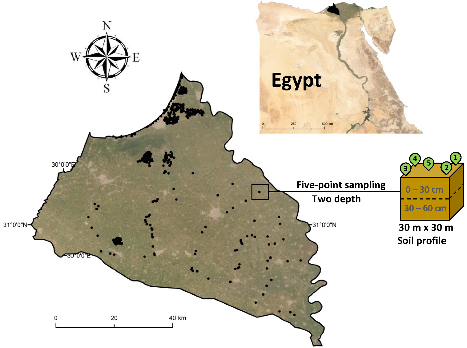
Figure 1. The case study area is located on the northwestern side of the Nile Delta of Egypt; black points are the location of soil samples that were used in the ML training and testing.
Remotesensing 15 01751 g001
Figure 2. A workflow illustration describes the analysis steps using various sources of remote sensing data inputs and ground truthing (soil sampling).
Remotesensing 15 01751 g002
Figure 3. The selected variables by filter methods of entropy, F-tests univariate feature ranking, Pearson, and Spearman.
Remotesensing 15 01751 g003
Figure 4. Regression learners training results with a subset of variables selected by feature selection methods; feature selection approaches were (i) recursive feature elimination (RFE), which included LR, RF, SVR, and BPNN; (ii) filter included entropy, Pearson, Spearman, and f-Test; and (iii) embedded included Lasso and RF; (A) coefficient of determination (R2), (B) Adjusted coefficient of determination (adj-R2), and (C) root mean square error (RMSE).
Remotesensing 15 01751 g004
Figure 5. The predicted soil salinity spatial distributions and the total of classified salinity share areas (%) at four (4) filter methods, (A) entropy method with RF learner; (B) Spearman method with RF learner; (C) Pearson method with RF learner; and (D) f-test method with RF learner.
Remotesensing 15 01751 g005
Figure 6. The predicted soil salinity spatial distribution and the total of classified salinity share areas (%) at four (4) wrapper methods, (A) BPNN method with RF learner; (B) LM method with RF learner; (C) RF method with RF learner; and (D) SVR method with RF learner.
Remotesensing 15 01751 g006
Figure 7. The predicted soil salinity spatial distribution and the total of classified salinity share areas (%) at two (2) embedded methods, (A) LASSO method with RF learner, and (B) RF method with RF learner.
Remotesensing 15 01751 g007
Table 1. Soil salinity classification and crop growth based on EC [78,79].
Salinity ClassSoil Salinity (dS/m)Effect on Crop Plants
Non-saline <2Negligible salinity effects.
Slightly saline 2–4Yields of sensitive crops maybe affected.
Moderately saline 4–8Yields of many crops are affected.
Strongly saline 8–16Only tolerant crops will survive.
Very strongly saline>16Only a few tolerant crops will survive.
Table 2. The stacked pre-processed raster variables of Sentinel-1 and Sentinel-2 that were used in ML training for mapping soil salinity in the study area.
DescriptionsSelected Variable
Sentinel-2, Band (b) selectionb2, b3, b4, b5, b6, b7, b8, b8A, b11 and b12.
Sentinel-2, IndicesWDVI, TNDVI, SAVI, NDWI, NDVI, MSAVI, MSAVI2, MNDWI, MCARI, IPVI, GNDVI, DVI, CI, BI and BI2.
Sentinal-1, sigma nought (δ0) dbVV and VH.
V V_ GLCMContrast_VV, Dissimilarity_VV, Homogeneity_VV, AngularSecondMoment_VV, Energy_VV, Entropy_VV,
MaximumProbability_VV, Correlation_VV, Mean_VV and StandardDviation_VV.
VH_ GLCMContrast_VH, Dissimilarity_VH, Homogeneity_VH, AngularSecondMoment_VH, Energy_VH, Entropy_VH,
MaximumProbability_VH, Correlation_VH, Mean_VH and StandardDeviation_VH.
Table 3. The recursive feature elimination base learners of LR, SVR, RF, LASSO, and BPNN.
LearnerSubsetted VariablesNo. of Subsetted VariablesRMSE
LR
  • band3, band6, band8, band8A, band11.
  • TNDVI, SAVI, NDVI, MSAVI, MSAVI2, MCARI, DVI, BI2,
  • VV, VH.
  • Contrast_VV, Dissimilarity_VV, Homogeneity_VV, Correlation_VV, Mean_VV, Standard_Deviation_VV.
  • Contrast_VH, Dissimilarity_VH, Angular_Second_Moment_VH, Energy_VH, Entropy_VH, Maximum_Probability_VH, Correlation_VH, Standard_Deviation_VH.
290.48174263
RF
  • band3, band4, band5, band7, band8, band12.
  • MNDWI, MCARI, SAVI, WDVI, BI2, NDVI.
  • Mean_VV, Homogeneity_VV, Maximum_Probability_VV, Angular_Second_Moment_VV, Energy_VV, Correlation_VV.
  • Mean_VH, Homogeneity_VH, Angular_Second_Moment_VH, Entropy_VH, Standard_Deviation_VH, Dissimilarity_VH.
240.52825744
SVR
  • band6, band7, band11.
  • BI2, WDVI, MNDWI, NDVI, DVI, CI, GNDVI.
  • VV.
  • Mean_VV.
  • Mean_VH, Dissimilarity_VH.
140.55513133
BPNN
  • band3, band4, band5, band6, band7, band12.
  • SAVI, MSAVI, MNDWI, MCARI, GNDVI, DVI.
  • VV.
  • Mean_VV.
  • Contrast_VH, Dissimilarity_VH, Mean_VH, Standard_Deviation_VH.
180.302719033
Table 4. The Feature selection and variables statistical assessment using embedded methods for soil salinity predictions.
LearnerSubsetted VariablesNumber of Subsetted VariablesRMSE
RFWDVI, TNDVI, SAVI, NDWI, NDVI, MSAVI, MSAVI2, IPVI, GNDVI, DVI, CI.
VV, VH
Mean_VV.
Mean_VH.
150.52825744
LASSOband3, band6, band8, band8A, band11, band12,
TNDVI, MNDWI, CI, BI2,
VV.
Contrast_VV, Dissimilarity_VV, Homogeneity_VV, Angular_Second_Moment_VV, Correlation_VV, Mean_VV.
Contrast_VH, Dissimilarity_VH, Homogeneity_VH, Angular_Second_Moment_VH, Maximum_Probability_VH, Correlation_VH, Angular_Second_Moment_VH, Maximum_Probability_VH, Correlation_VH.
230.5093330
Disclaimer/Publisher’s Note: The statements, opinions and data contained in all publications are solely those of the individual author(s) and contributor(s) and not of MDPI and/or the editor(s). MDPI and/or the editor(s) disclaim responsibility for any injury to people or property resulting from any ideas, methods, instructions or products referred to in the content.