Abstract
A stable and reliable cloud detection algorithm is an important step of optical satellite data preprocessing. Existing threshold methods are mostly based on classifying spectral features of isolated individual pixels and do not contain or incorporate the spatial information. This often leads to misclassifications of bright surfaces, such as human-made structures or snow/ice. Multi-temporal methods can alleviate this problem, but cloud-free images of the scene are difficult to obtain. To deal with this issue, we extended four deep-learning Convolutional Neural Network (CNN) models to improve the global cloud detection accuracy for Landsat imagery. The inputs are simplified as all discrete spectral channels from visible to short wave infrared wavelengths through radiometric calibration, and the United States Geological Survey (USGS) global Landsat 8 Biome cloud-cover assessment dataset is randomly divided for model training and validation independently. Experiments demonstrate that the cloud mask of the extended U-net model (i.e., UNmask) yields the best performance among all the models in estimating the cloud amounts (cloud amount difference, CAD = −0.35%) and capturing the cloud distributions (overall accuracy = 94.9%) for Landsat 8 imagery compared with the real validation masks; in particular, it runs fast and only takes about 41 ± 5.5 s for each scene. Our model can also actually detect broken and thin clouds over both dark and bright surfaces (e.g., urban and barren). Last, the UNmask model trained for Landsat 8 imagery is successfully applied in cloud detections for the Sentinel-2 imagery (overall accuracy = 90.1%) via transfer learning. These prove the great potential of our model in future applications such as remote sensing satellite data preprocessing.
1. Introduction
Clouds can affect the Earth’s radiation balance through absorption and scattering [1], and then affect the atmospheric environment and climate change [2]. However, for passive remote sensing, especially quantitative remote sensing retrieval, clouds are troublesome noises that need to be accurately identified and masked before extracting the land-related (e.g., land use classification, urban building extraction et al.) and atmospheric (e.g., aerosol or gas retrieval) parameters [3,4,5]. Clouds are everywhere, covering more than half of the globe each year, especially in tropical areas [6,7,8]. In addition, both the shapes and amounts of clouds are changing over time, leading to diverse mixed pixels with the underlying surfaces, significantly increasing the detection difficulties [5].
To address this issue, a series of classical cloud detection algorithms have been proposed successively over the years. The most popular one is the fixed threshold approach, which is simple and easy to operate, such as those developed for the International Satellite Cloud Climatology Project (ISCCP) [9,10,11], Clouds from the Advanced Very High Resolution Radiometer (AVHRR) (CLAVR) [12], and AVHRR Processing scheme Over cLouds, Land and Ocean (APOLLO) [13,14]. Besides them, a lot of efforts have been made to help improve cloud detection, especially those clouds over bright surfaces, e.g., Irish adopted multiple spectral indices and band ratios to enhance the difference between clouds and bright surfaces [15], and then established an Automatic Cloud Cover Assessment (ACCA) system [16]. Hazy Optimized Transform (HOT) was designed to detect haze apart from clouds [17,18], and a whiteness index to exclude cloudy pixels by considering the different reflectance changes in the visible band compared to other surface types [19]. Hegarat-Mascle and Andre introduced the green and Short Wave Infrared (SWIR) channels along with Markov Random Field (MRF) to detect different types of clouds [20]. Zhu and Woodcock proposed the Fmask algorithm by setting up a series of spectral tests that integrated the advantages of previous different threshold methods to identify clouds for Landsat imagery [21]. Sun et al. developed a dynamic threshold algorithm upon radiative transfer simulation by constructing a prior surface reflectance database to improve cloud detection by minimizing the influence of mixed pixels [4]. Zhai et al. calculated and combined the spectral indices and cloud and cloud shadow indices to identify clouds for multispectral and hyperspectral optical sensors [22].
Despite unique advantages, threshold methods still suffer from great challenges, especially for those sensors with high spatial resolutions and few spectral channels, making it difficult to find a proper threshold to separate clouds from the complex underlying surfaces [16,23,24]. They also face difficulties in bright areas, such as bare land, snow, and ice areas, due to the similarity in reflectance from visible to near-infrared bands. Temperature-based tests also often fail with inversion effects in high-latitude areas [25]. For special areas such as vegetation and desert, additional thresholds varying with the geometric position should be considered and designed [13]. These surface conditions make the detection logic of the threshold methods more complex [16]. Therefore, “clear restoral tests” are needed to avoid misclassification [26] and testing areas of ice and snow also adds uncertainty to the results [27].
In recent years, machine learning (ML) has made great progress in improving cloud detection for sensors with fewer channels due to its strong data mining capability from a large number of input potential features [28]. The fundamental reason for the performance improvement is the ability to optimize the extracted features in the loop [29]. The specific step is to find the optimal classifier through a series of nonlinear transformations of the input data. An increasing number of cloud mask studies have been performed by adopting different ML approaches, e.g., support vector machine (SVM) [30], neural network (NN) [31], decision tree [32], and random forest [33]. However, most ML methods work in pixel-by-pixel classification mode, which cannot consider the context and global information of clouds. In contrast, deep learning (DL) models can combine spectral and spatial information simultaneously and have been widely used in the fields of Computer Vision (CV) and medicine, such as face recognition [34,35], segmenting and tracking on 3D video sequences [36], and extracting and curating individual subplots [37]. DL is also particularly suitable for remote sensing classification tasks. Convolutional Neural Network (CNN) is the most widely used in remote sensing classification [38,39] and object detection [40,41]. CNN models can extract different features, which have been preliminarily applied to cloud detection, e.g., Goff et al. combined the Simple Linear Iterative Clustering (SLIC) algorithm and deep Convolutional Neural Network (CNN) to identify clouds for SPOT imagery [42]. Zi et al. designed a double-branch PCA Network (PCANet) utilized by SLIC and Conditional Random Field (CRF) to recognize clouds for Landsat 8 imagery [43], deep pyramid network [44], SegNet [45], U-net [29,46], and Multi-scale Convolutional Feature Fusion (MSCFF) [47]. The CNN model has a strong generalization ability and is not easy to overfit [48]. Although the CNN model can achieve high accuracy, training the CNN model requires a large number of pixel-level classification labels, and the acquisition of these labels is very time-consuming and laborious. To solve this problem, a generative adversarial network (GAN) can be used, which only needs block labels emerged [49]. GAN is a weakly supervised classification method, including two parts: generative model and discriminative model. The generation model can generate image data consistent with the distribution of input data, and the discrimination model can determine the category of image. GAN has been successfully applied in image conversion [50,51], and has also been adopted for many remote sensing applications [52,53,54]. For cloud detection, the generative model can generate simulated cloudless images, then obtain cloud detection results through the difference with cloud images, and finally, use a small number of pixel-level labels for fine tuning [55]. Wu et al. introduced the self-attention mechanism into GAN(SAGAN) to extract this difference [56]. Zou et al. added a cloud matting network to learn and train the fake cloud images GAN generated. However, GAN generally has problems, such as training difficulty and mode collapse [57], which mean that GAN has not been applied on a large scale in remote sensing. On the other hand, images can be seen as two-dimensional sequences with location information. Based on this idea, some Natural Language Processing (NLP) models are applied to CV, such as transformer. Vision Transformer (ViT) consists of embedding, an encoder, and an MLP head. The embedding layer can transform the image into a token sequence, then encodes the token sequence and last outputs the probability vector of the image classification [58]. When the training data are sufficient, the model performance of ViT will exceed that of CNN and can obtain a better transfer effect in downstream tasks. To better adapt to semantic segmentation tasks and reduce the amount of computation, Swim Transformer designs a structure similar to CNN to gradually reduce the feature map resolution and limits the global self-attention to a certain area compared with ViT. Finally, results are very good under 15 million images training. Furthermore, in order to better identify objects with large size and different directions in remote sensing images, Wang et al. used the MillionAID dataset to pretrain remote sensing backbones, proving that it is practical in the downstream tasks of remote sensing [59], and developed a transformer model specifically applied to remote sensing [60]. However, the transformer models need lots of data for training, and require high hardware requirements, which is still in the development stage.
When the satellite has not been launched, or the band range of the satellite is narrow, such as GF-1 or Proba-V satellite, it is difficult to design a cloud detection algorithm and there is a lack of sufficient verification data. In this context, using the wealth of information contained in the existing labeled datasets, it is possible to transfer previous knowledge about the problem between similar satellites. Mateo-García et al. proved that the cloud detection model based on deep learning could be transferred between satellites with similar spectral and spatial information [61]. Li et al. used Landsat 8 data to train the generating adversarial network (GAN), which has good transferability to Sentinel-2 images [62]. Since the CNN model is still the most widely used deep learning model, the objective of this research is to increase both the accuracy and efficiency in cloud detection for Landsat 8 imagery by adopting a variety of derivative-developed models based on the original CNN model, including the Fully Convolutional Networks (FCN) [63], U-net [64], SegNet [65], together with DeepLabv3+ [66] models. Here, we trained each model using the global cloud cover assessment database provided by the United States Geological Survey (USGS) and qualitatively comprehensively evaluated, compared, and discussed the performance, advantages, and uncertainties of the different models in cloud detection over varying surfaces from both qualitative and quantitative perspectives. Last, the best-performing one was successfully transferred to the latest released Sentinel-2 imageries via transfer learning.
2. Data Materials
Landsat is one satellite mission (e.g., 15–120 m, 4–11 bands) which was widely used in monitoring land change, heat island effects, and air quality. The Landsat series has launched a total of nine satellites, of which the Landsat 7 satellite was placed into orbit mode in April 2022, and Landsat 8 and 9 satellites launched in February 2013 and September 2021, respectively, and has become the primary data source for future continuous Earth observations. The Landsat 8 satellites carry two sensors, including the Operational Land Imager (OLI) and the Thermal Infrared Sensor (TIRS), and achieve global coverage every 16 days.
Sentinel-2 has two satellites called Sentinel-2A and Sentinel-2B, which launched in June 2015 and March 2017, respectively. Both carry a MultiSpectral Instrument (MSI) and cover 13 spectral channels, from visible and near-infrared to short-wave infrared, at different spatial resolutions. Sentinel-2 data are the only data with three bands in the red-edge range, which is very effective for monitoring vegetation health information [67]. Different from Landsat 8 and 9 data, Sentinel-2 data have a very diverse set of bands, showing large differences from visible to near-infrared channels (Figure 1), and thus are selected to test the applicability of transfer learning. Table 1 shows detailed information about Landsat and Sentinel imagery.

Figure 1.
Comparison in spectral response functions between Landsat 8 and Sentinel-2A satellites.

Table 1.
Detailed information about the Landsat 8 and Sentinel 2 satellites.
Landsat 8 Biome Cloud Mask Validation database (U.S. Geological Survey, Reston, VA, USA, 2016) were selected to establish the cloud detection model for Landsat 8 imagery. It includes 96 global scenes covering all surface types, including barren, water, wetlands, forest, grass/crops, shrubland, urban, and snow/ice [68]. Here, clouds and non-clouds of the scenes over different underlying surfaces were selected using the stratified sampling method and used for training (48 scenes) and validation (48 scenes) data (Figure 2). The Sentinel-2 Cloud Mask Catalogue dataset was employed, which consists of 513 subscenes (259 Sentinel-2A images and 254 Sentinel-2B images) with 1022 × 1022 pixels evenly distributed throughout the world [69]; they were employed and used to evaluate the performance of transfer learning for Sentinel-2 imagery.

Figure 2.
Geolocations of global Landsat 8 Biome training (marked in red colors) and validation (marked in pink colors) images. Background map is MODIS land use cover product in 2019.
3. Models and Methods
3.1. Convolutional Neural Network
CNN is a model that acquires the ability to learn by making reasonable assumptions about images (such as local correlations) [70], which is similar to artificial neural networks. In the field of image classification and recognition, the input is an image with the size of m × n × k, where m, n, and k are the height, width, and number of the image channels, respectively. The output is a vector with the dimension of c, where c is the number of classification categories. Each element in the vector represents the probability of the corresponding category. Differently, in the image segmentation task, the input and output embrace the same height and width. The CNN model usually experiences two steps, e.g., (1) it runs the downsampling continuously and collects the image information of various scales using the convolutional layer and pooling layer; (2) the fully connected layer is applied to integrate the information for the classified output. The extensive application of the specific CNN models appreciates the usage of these two working steps in the image classification and recognition field.
The convolutional layer is similar to the traditional filters such as the mean filter and Gaussian filter:
where i and j present the position of pixels, I is the input image or feature map, and K is the m × n × l kernel. The number of kernels, d, is determined by the channels of the output feature maps. It is selected manually when constructing the network architecture. Another layer is named the pooling layer, including the max pooling, and mean pooling refers to the downsampling towards each area. The downsampling can be operated to exploit a wider range of features, reduce the input size of the next layer, decline the amount of calculation, and diminish the number of parameters. In addition to the above two layers, other layers can be incorporated together in some typical CNN models, such as VGG-16. Figure 3 illustrates the structure of VGG-16, which employs not only the convolutional layer and pooling layer but also the fully connected layer. However, only the convolution layer and pooling layer are most used in the field of image segmentation.

Figure 3.
The VGG-16 architecture.
3.1.1. FCN
The FCN model is the precursor which extends the end-to-end and pixels-to-pixels CNN to the image semantic segmentation [63]. The FCN architecture schematic is presented in the FCN model, and the fully connected layer is substituted into the convolutional layer to input images regardless of their size (Figure 4a). Then, the size of the feature map is gradually restored by skip structure and deconvolution layer. The skip connections combine the feature map undergoing the convolution and pooling operations with the corresponding upsampling data to cover the lost spatial information and restore the image details. Almost all CNN models of image segmentation apply this structure. According to the stride of the deconvolution layer, the FCN model can be divided into FCN-8s, FCN-16s, and FCN-32s, etc. Theoretically, more detailed spatial information contributes to a better classification result. Therefore, the FCN-2s were selected to represent the FCN model.
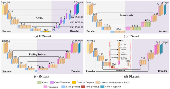
Figure 4.
Framework for (a) FCNmask, (b) UNmask, (c) SNmask, and (d) DLmask, respectively.
3.1.2. U-Net
Based on the thought of the FCN model, the U-net model is developed to improve its basic structure [64] (Figure 4b). Several differences can be summarized as follows: (1) The U-net model is completely symmetrical. Its decoder is processed with the convolutional layer, which can better seize the detailed information. Diversely, the FCN model has sole upsampling layers in the decoder. (2) In the U-net model, each channel of the images is concatenated by the skip connection’s structure, and the number of channels is raised. The FCN model is solely the summation of the corresponding pixels.
The encoder consists of 3 × 3 convolutions, each followed by a Rectified Linear Correction Unit (ReLU) and a 2 × 2 max pooling operation with downsampling with stride 2. Each step in the decoder consists of upsampling the feature map and concatenating it with the corresponding feature map from the encoder. U-net combines deep and shallow image information through skip structure, and in the upsampling part, the contextual information is sent to higher-resolution layers.
3.1.3. SegNet
Similarly, the SegNet model also exhibits a completely symmetrical structure [65] (Figure 4c), which is highlighted by the fact that this model saves the index values of the max pooling. After each pooling operation, the relative position of the maximum value of the element, namely the index value in the pool, is saved by a 2 × 2 matrix. In the decoder part, each encoder corresponds to a decoder. The index value pre-served in the encoder is applied in the decoder. Notably, each 2 × 2 matrix loses three weights which cannot be recovered after the pooling operations. The size of the feature map is zoomed in twice, but the position of the largest element in the pooling can be gained in the upsampling layer. Then, the maximum value of the input feature map is placed according to the index. The rest positions are padded with zero, and their weight is zero correspondingly. In order to fill in the missing content, the convolutional layer is employed in the SegNet model. Overall, training and learning are not required in this upsampling, and the number of parameters can be cut down effectively.
3.1.4. DeepLab
DeepLab models introduce atrous convolution, which can increase the receptive fields while the size of the feature map is fixed. Despite the increment of the receptive fields on the premise of unchanging the size of the feature map, utilizing the atrous convolution once to extract multi-scale target information is limited. The information of small-scale feature maps cannot be reflected by that of large-scale maps, and the adoption of the atrous convolution to exploit all feature maps is very redundant. Therefore, the atrous convolution is often employed accompanied by the convolutional and pooling layers, which can diminish the number of the pooling and upsampling layers, and the information losses can be cut down. In the DeepLabv1 [71], some convolutional layers are substituted by the atrous convolution based on the VGG-16. DeepLabv2 [72] features the addition of the Atrous Spatial Pyramid Pooling (ASPP), which can gain more layers of diverse dilated rates to enhance the ability to recognize the same objects of different sizes. As depicted in Figure 4d, the DeepLabv3+ [66] applies the encoder and decoder structure, and the ASPP is inserted into the decoder, which is the most accurate DeepLab model at present.
In this study, based on the initial frameworks of these traditional CNN models, more changes are made, e.g., the use of multiple spectral discrete channels with additional normalization and newly added cropping layers to block remote sensing images, leading to four extended models for Landsat remote sensing images, named FCNmask, UNmask, SNmask, and DLmask, respectively.
To describe the complexity and running speed of the CNN models, the parameters amount and floating-point operations per second (FLOPs) can be used (Table 2). The complexity of the model is expressed by the parameter amount. In contrast, the reasoning speed is replaced by FLOPs. It should be noted that due to various factors, such as computer hardware, the number of FLOPs cannot accurately reflect the actual speed [73].
Table 2.
The parameters amount and FLOPs for CNN models. 1 M = 106, 1 G = 109.
3.2. Model Training and Validation
3.2.1. Model Training
The model training experiences three steps, including data normalization, image clipping, and optimizer and initialization method settings. We converted the DN values into top-of-atmosphere (TOA) reflectance for data normalization. The size of patches and overlap was maintained at the baseline conditions of 256 × 256 and 100 separately for training data. These patches were used for data augmentation, and there is a 50% probability of horizontal or vertical flips. The total iterations were about 6000, and the batch size was 8. The Adam optimizer was employed for training. The activation functions were ReLU, and batch normalization was set at a momentum of 0.9. Xavier’s normal initialization method was used for all the convolutional layers. To avoid overfitting problems, dropout probability and L2-regularization were both fixed at 0.5 in training models. We trained the efficiency of the DL cloud detection model based on the computer with Intel Core i7-10875H, 16 GB RAM, and Nvidia GTX 2060, using Keras 2.3.1 and TensorFlow 2.1.0. Figure 5 shows the performance of different models during training.

Figure 5.
The optimization curves of accuracy for different models.
Notably, although various measures were taken during the training process, it is evident in Figure 6 that the overfitting phenomenon still exists on the Sentinel-2 dataset. In order to address this problem, an early stop strategy was adopted, and the epoch equal to 5 was selected for the investigation.

Figure 6.
The training and validation accuracy on the Landsat 8 and Sentinel 2 datasets for the UNmask model.
3.2.2. Model Validation
Here, the cloud amount difference (CAD) is used by calculating the difference between the predicted and the true cloud masks [4]. Moreover, three typical evaluation indices, i.e., Accuracy, Recall, and Precision, are selected to represent the overall accuracy, omission error, and commission error of the model clarifications, respectively. They are calculated (Equations (2)–(5)) through the confusion matrix using four quantities: true positives (TP), false negatives (FN), true negatives (TN), and false positives (FP). In the cloud detection task, the positive class is clouds, while the negative class is non-clouds. Last, the balanced F score (F1-score), defined as the harmonic average of Precision and Recall rates, is also adopted to measure the performance of classification.
McNemar’s test statistic is used to estimate whether two models are significantly different [74]. Statistics χ2 depends on the chi-square distribution, where b is the model 1 correct prediction and model 2 wrong prediction, and c is the model 1 wrong prediction and model 2 correct prediction. The larger the χ2, the greater the difference between the two models.
3.2.3. Transfer Learning
Theoretically, different sensors need their own data samples for model training; however, manually labeling and sketching a large number of data samples for any sensor takes huge time and effects. Under such background, the idea of transfer learning is proposed [75], that is, to find a balance between two assumptions: (1) the training set is adequate to represent the potential data distribution, (2) the test data originate the same distribution. Transfer learning is also applicable to cloud classification among different sensors with similar designs in spectral channels, e.g., Landsat 8 and Sentinel-2 (Figure 1), assuming that the available training samples for the former can be applied to the latter.
For transfer training, we labeled data from the source domain and unlabeled data from the target domain. Considering the DL model for cloud detection has already been trained for Landsat 8 imagery, first, we used the Landsat 8 data to train the model, then converted the Sentinel-2 data into Landsat 8 data; last, we obtained the Sentinel-2 result. Note that although these two satellite sensors are similar, there are still spectral differences that needed be corrected first. Here, we adopted the spectral convolution method [76] via the spectral response functions (SRF) to eliminate such differences since the spectral overlap between signals in two domains exists:
where indicates the coefficient of conversion for band I of Sentinel-2. is the Sentinel-2 spectral response function for the band i. is the Landsat 8 spectral response function for the band j. bandimin and bandimax are the minimum and maximum wavelengths where is greater than zero.
4. Results and Discussion
4.1. Landsat 8 Cloud Detection Results
Figure 7 illustrates the typical examples and the corresponding cloud distributions detected by four involved DL models under diverse underlying surfaces. The cloud detection results are basically consistent with the true cloud distributions; specifically, clouds over densely vegetated areas can be accurately classified for all models of their large differences in reflectance (Figure 7a–e). Furthermore, good classification results are also observed in other dark surfaces, such as the ocean (Figure 7a), coastal waters (especially the land–sea junction) (Figure 7b), and inland water (Figure 7c). As the surface brightens, most DL models still can identify well different types of clouds over, e.g., the urban areas, especially broken clouds near or above the buildings (Figure 7e), as well as the barren areas (Figure 7f), especially the thin clouds over the desert (pointed by orange arrows), showing few omissions and misclassifications. Despite overall good results, some differences in details exist among the models due to the differences in algorithm designs, e.g., it is easier for the FCNmask model to miss small and broken clouds than others.
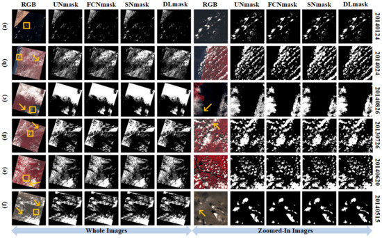
Figure 7.
Examples of full-scene and zoom-in standard-false-color (RGB: 4-3-2) images and cloud detection results from (a–f) dark to bright surfaces for Landsat 8 imagery using the UNmask, FCNmask, SNmask, and DLmask, respectively. The right-side annotations indicate the acquisition time (yyyymmdd, where yyyy = year, mm = month, dd = day).
Figure 8 illustrates the performance of different CNN-derived DL models in detecting clouds on varying bright surfaces with great challenges due to their similar spectral characteristics compared to clouds. For the clear-sky surfaces, most models rarely misclassify bright surface-type pixels into clouds over artificial constructions (Figure 8a), minerals and rocks (Figure 8b), Gobi and deserts (Figure 8c,d), as well as high-altitude mountains (Figure 8e) and polar regions (Figure 8f) covered by temporary and permanent snow and ice (Figure 8e,f), showing low commission errors (pointed by red arrows). By contrast, for cloudy regions, large differences are seen among these models, e.g., in general, UNmask can more accurately capture both the shape and edge of the clouds, which is more consistent in the spatial distribution with the real image, especially for thin and broken cloudy scenes.

Figure 8.
Same as Figure 7, but the bright surfaces: (a) urban, (b–d) bare and desert, (e–f) ice and snow, where orange and red arrows point to cloudy and clear-sky surfaces.
SNmask shows a similar performance compared to UNmask in most situations, showing few cloud omissions and misidentifications. This benefits from the preserved index value of the max pooling [65]. FCNmask can easily miss the broken clouds in the images due to the limitations of the deconvolution layer used, which will lose some extremely high values [77]. DLmask misses the most clouds over the bright surfaces, especially for the ice and snow surfaces (Figure 8f), because the atrous convolution for the model core has kernel gaps, where only part of the pixels are used for calculation, resulting in a loss of information continuity. In addition, the gained uncorrelated remote spatial information hinders the detection process, while clouds are most locally related [78].
4.2. Quantitative Accuracy Evaluation
4.2.1. Overall Performance and Operating Efficiency
First, we validate the predicted cloud amount by different CNN-derived models against the real cloud amount (Figure 9). Overall, the percentages of the cloud cover calculated by these models are basically consistent with those of the USGS manual generations (e.g., slope = 0.92−0.96, and R2 = 0.9−0.97). Among these models, the DLmask model shows the worst performance in estimating the cloud amount with the lowest correlation and smallest slope, showing the largest MAE value. In general, the FCNmask and SNmask models show comparable performance with similar evaluation indices. By contrast, the UNmask model is the most accurate one with the strongest slope, highest R2, and smallest MAE (~2.2%) values, which can be of great importance for future Landsat image screening and selection. It should be noted that, overall, all the models tend to underestimate the cloud amount (i.e., CAD < 0), especially for the FCNmask model (CAD = −0.67%), which is mainly attributed to the easy omission of small and broken clouds.

Figure 9.
Comparison in cloud amount between Landsat 8 Biome validation dataset and different CNN models: (a) UNmask, (b) FCNmask, (c) SNmask, and (d) DLmask.
Next, we evaluate the overall accuracy of different DL models in cloud classification (Table 3) and discuss their performance on different surface types (Figure 10). All four models have good evaluation indices exceeding 90%. Nevertheless, the performance of the four models is quite different according to McNemar’s test statistics χ2 (Table 4). Under the circumstances, the F1-score and overall accuracy indices of the UNmask model are equal to 94.1% and 94.9%, respectively, which are superior to the other three models. The UNmask model and FCNmask model are biased by the Biome datasets, leading to the imbalance between Recall and Precision index and a sub-optimal F1-score. Notably, in terms of Recall and Precision metrics, the Recall value of the FCNmask model is much higher than Precision because of the fixed threshold, which is more likely to misidentify clouds as non-clouds. In general, the UNmask model shows the best performance with all the highest evaluation indices among these CNN-derived models.
Table 3.
Statistics describing the evaluation results using confuse matrix for different models.

Figure 10.
Model performance in cloud detection for Landsat 8 imagery over different land-use types in terms of (a) Accuracy, (b) Recall, (c) Precision, and (d) F1-score.
Table 4.
McNamara’s test statistics χ2 describing the evaluation results for different models.
All surface types can be divided into three groups: dark surface (water and wetlands), vegetated surfaces (forest, grass/crops, shrubland), and bright surface (urban, barren, and snow/ice). For dark surfaces, all indicators are very balanced. The overall accuracy and F1-score indices surpass 95%, and the Recall and Precision of the four models are close, illustrating that there are almost no obvious misclassification and omission errors. The excellent performance is attributed to the distinctive spectral differences between dark surfaces with low surface reflectance and high-reflecting clouds. It is noteworthy that the Precision is less than the Recall for the DLmask model, indicating that some clouds may be missed.
In the vegetated areas, the overall accuracy index is greater than 93% for all models. For all vegetated surface types, the UNmask model is superior to others for all indicators. With respect to the forest surface type, grass/crops surface type, and shrubland surface type, the overall accuracy is 93.6%, 97.3%, and 94.5%, and the F1-score is 94.2%, 96.8%, and 93.5%, respectively. Notably, for forest and shrubland, the Recall values of the four models are much higher than the Precision values, demonstrating that many clouds are missed detected.
For bright surfaces, the performance of the UNmask model ranks in the first position. Urban surface embraces the best performance for all the models. The F1-score and overall accuracy are up to 97.5% and 97.2%, respectively, under the simulation of the UNmask model. The ignorable difference demonstrates that these models are robust without obvious cloud omissions and misidentifications, which can be attributed to two aspects: clouds are primarily distributed in dark surfaces such as vegetated and lake areas, which are easier for detecting clouds; these models grasp the spectral characteristics and differences by fully training datasets consisting of cloud pixels and clear sky pixels from different surfaces. As for the barren surface types, the Recall is higher than the Precision, indicating that clouds are often missed. However, an opposite phenomenon is observed over snow/ice surfaces. In summary, the UNmask model shows the best performance among different surface types from Figure 10.
4.2.2. Model Comparison and Efficiency Analysis
Here, we use the same validation source Landsat 8 biome reference masks to compare with some algorithms (Table 5). It is noteworthy that the reference images used are not the same, which may lead to unfair accuracy comparison. The results indicate that the UNmask algorithm performs better than traditional threshold-based models, such as the Landsat 8 Surface Reflectance Code (LaSRC) algorithm, the ACCA, Artificial Thermal (AT)-ACCA, and Fixed Temperature (FT)-ACCA algorithms, the C implementation of Function of Mask (CFmask) algorithm [45,68], the CDAL8 algorithm [24], and the FMask algorithm [29,47,79]. UNmask is an improvement on our previously developed RFmask model [33] due to a higher capacity for deep learning; in addition, it is superior or comparable to other developed ML or DL algorithms such as the See5 algorithm [68], SegNet [45], and MSCFF [47]. In general, our Unmask model outperforms most models developed in previous studies; in particular, its advantages of rapid automation and transfer learning have broad prospects for future applications.
Table 5.
Comparison in cloud detection with previous studies using the same Landsat 8 Biome cloud validation mask.
The data preprocessing includes data load, band combination, and radiometric calibration, taking a total of about 12.0 ± 1.6 s, and the main time-consuming steps of this process are the layer stack. It is noteworthy that the prediction time is independent of the model type, costing 25.6 ± 3.4 s. The cloud detection results are saved as GeoTiff files, which use 3.4 ± 1.0 s. The above results are based on a single-threaded implementation. A multi-threaded implementation that simultaneously loads/saves and processes data will reduce the total processing time, making it close to the predicted time. The total time is 41 ± 5.5 s, which is much faster than pixel-by-pixel classification, indicating that it has obvious application prospects.
4.2.3. Impacts of Threshold Setting on Cloud Detection
Last, the influence of varying thresholds on the cloud detection results is also analyzed. The Recall swiftly rises, and the Precision marginally declines when the threshold is low (Figure 11a). As the threshold is augmented, the increase in the Recall and the decrease in the Precision are basically the same. Then, the Precision reduces rapidly, and Recall increases slowly when the threshold is high. These unique tendencies reflect that to find an appropriate threshold, a trade-off between Recall and Precision should be involved. Considering that the F1-score is a harmonic mean between the Recall and Precision, the F1-score accompanied by the overall accuracy is specified to investigate the effect of the thresholds.
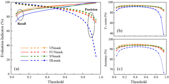
Figure 11.
Effects of varying thresholds on different CNN models using Landsat 8 Biome dataset in terms of (a) Recall and Precision, (b) F1-score, (c) Accuracy.
The impact of different thresholds on the F1-score is shown in Figure 11b. In general, the F1-score exhibits a trend of rising first and then depreciating. Comparatively, the evolution of the UNmask, FCNmask, and SNmask model changes more smoothly due to the slow variation of the Recall and Precision, while the DLmask is opposite completely. The overall accuracy behaves similarly to the F1-score, as observed in Figure 11c. The tendency of the increasing first and then decreasing of the F1-score and overall accuracy highlights that an optimal threshold exists. For these models, a threshold in the range of 0.2–0.7 is recommended. For the DLmask model, a threshold less than 0.6 is considered suitable. Within this range, the optimal threshold can be found from the intersection of the Recall and Precision curves in Figure 11a. The optimal threshold is close to 0.4 for the UNmask and FCNmask models and is close to 0.5 for the SNmask and DLmask models.
4.3. Transfer Learning Cloud Detection for Sentinel 2 Imagery
4.3.1. Overall Performance and Operating Efficiency
Additionally, UNmask was applied to the cloud detection for Sentinel 2 through transfer learning, and it performs well over dark surfaces, such as the ocean (Figure 12a), the boundary between land and sea (Figure 12b), and most of the thin and broken clouds can be correctly detected. Additionally, the model shows superior performance in vegetated areas (Figure 12c–e). For the bright surfaces, the distribution of detected clouds agrees well with the original image over urban buildings (pointed out by red arrows in Figure 12d). Moreover, expected cloud detection results are also observed in the bare rock and bare land (Figure 12e,f), even in the presence of mountain snow (Figure 12b indicated by red arrows). For Sentinel-2, the overall accuracy, F1-score, Recall, and Precision are 90.1%, 90.2%, 89.1%, and 91.4%, respectively. Nevertheless, this is acceptable compared with the huge time and energy consumption caused by reconstructing or retraining the model, especially largely limited to the available cloud validation mask data for different satellite sensors.
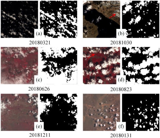
Figure 12.
Examples of standard-false-colour (RGB: 8-4-3) images and cloud detection results from (a–f) dark to bright surfaces for Sentinel 2 imagery. The acquisition time is below the image (yyyymmdd, where yyyy = year, mm = month, dd = day).
4.3.2. Model Comparison
We also used Fmask 4.0 algorithm [80] and the GAN-CDM-6 model [62] to predict the results of the Sentinel-2 Cloud Mask Catalogue dataset, and the results are listed in Table 6. From the perspective of model performance, the GAN-CDM-6 model has the highest indicators (Accuracy = 92.5%, F1 = 92.9%), followed by UNmask and the lower Fmask 4.0 algorithm. Although the GAN-CDM-6 model has the advantage of higher accuracy than Unmask model and only requires block labels, the complexity of the training model is higher, indicating that the GAN-CDM-6 model convergence is time-consuming and difficult (FLOPs = 201.66 G, Iterations = 1,000,000). In contrast, the UNmask model can achieve an accuracy (Accuracy = 90.1%, F1 = 90.2%) close to that of the GAN-CDM-6 model, and the difficulty of model training is also low (FLOPs = 28.11 G, Iterations = 6000), which is more conducive to practical application.
Table 6.
Average accuracy, FLOPs, and Iterations indicators of different methods on 512 images in Sentinel-2 Cloud Mask Catalogue dataset for Fmask 4.0, UNmask, and GAN-CDM-6 models.
5. Conclusions
Traditional threshold cloud detection methods mainly use spectral properties and hardly consider the spatial autocorrelation of target objects, especially for those satellites (e.g., Landsat) with high spatial resolution but few channels, significantly increasing the difficulties in detecting thin and broken clouds, particularly those over the bright surfaces. Therefore, this study employed four typical CNN-derived DL models, i.e., FCNmask, UNmask, SNmask, and DLmask, which are based on various convolution kernels, pooling, and skip connections to extract more different scale spatial features and to improve cloud detection for Landsat 8 imagery. The USGS Landsat 8 Biome Cloud Validation Masks covering diverse underlying surfaces were collected to train and validate the models. The top-of-atmosphere reflectance from visible to short-wave infrared wavelengths after radiometric calibration was used as the model input. Last, we also investigated whether the reconstructed cloud detection model for Landsat 8 imagery can be transferred, learned, and applied to Sentinel-2.
Experiments demonstrate that the estimated cloud amount has a good linear relationship with the validation cloud masks, especially the UNmask model (R2 = 0.97) with the smallest estimation uncertainties (i.e., MAE = 2.2%). This model also can most accurately identify the cloud distribution with an overall accuracy of 94.9% and an F1-score of 94.1% for Landsat 8 imagery. In general, the UNmask model has good adaptability over different underlying surfaces, with the best performance over urban areas (overall accuracy = 97.5%, and F1-score = 97.2%). In addition, the model also works well on brighter surfaces such as barren and snow/ice surfaces, e.g., overall accuracy = 94.6% and 89.3%, and F1-score = 93.4% and 82.0%, respectively. Furthermore, the efficiency test shows that the model is fast, which only takes a total of 41 ± 5.5 s on average to finish one-scene cloud detection. Finally, we transferred the UNmask model to the Sentinel-2 imagery and found that it has good classify accuracy (e.g., CAD = 5.85%, overall accuracy = 90.1%) and efficiency in both dark and bright surfaces, which further illustrates the robustness of our model and its great significance for quantitative application ability in the future.
Although the deep CNN model has significant advantages, some improvement methods can be considered for Landsat cloud detection. The digital elevation model and global surface coverage map can be included as the additional bands by layer stack, which can design appropriate thresholds for different surface types and altitudes to improve the performance of the model. Moreover, new architectures can be designed to improve cloud detection by considering the image texture and shape information.
Author Contributions
Conceptualization, J.W.; methodology, S.P.; software, S.P.; validation, S.P., Y.T. and Y.M.; formal analysis, J.W. and S.P.; investigation, S.P., Y.T. and Y.M.; resources, S.P.; data curation, S.P. and Y.T.; writing—original draft preparation, S.P.; writing—review and editing, J.W.; visualization, Y.T. and Y.M.; supervision, L.S.; project administration, L.S.; funding acquisition, L.S. All authors have read and agreed to the published version of the manuscript.
Funding
This research was funded by the Introduction plan of high-end foreign experts (Grant No. G2021025006L) and the National Natural Science Foundation of China (Grant No. 42271412).
Data Availability Statement
Landsat 8 Biome Cloud Mask Validation database (U.S. Geological Survey, 2016, available at https://landsat.usgs.gov/landsat-8-cloud-cover-assessment-validation-data (accessed on 1 January 2023). The Sentinel-2 Cloud Mask Catalogue dataset (available at https://zenodo.org/record/4172871#.YYI4BmBByUk (accessed on 1 January 2023)).
Conflicts of Interest
The authors declare no conflict of interest.
References
- Harshvardhan; Randall, D.A.; Corsetti, T.G. Earth Radiation Budget and Cloudiness Simulations with a General Circulation Model. J. Atmos. Sci. 1989, 46, 1922–1942. [Google Scholar] [CrossRef]
- Ramanathan, V.; Cess, R.D.; Harrison, E.F.; Minnis, P.; Barkstrom, B.R.; Ahmad, E.; Hartmann, D. Cloud-Radiative Forcing and Climate: Results from the Earth Radiation Budget Experiment. Science 1989, 243, 57–63. [Google Scholar] [CrossRef] [PubMed]
- Sun, L.; Wei, J.; Wang, J.; Mi, X.T.; Guo, Y.M.; Lv, Y.; Yang, Y.K.; Gan, P.; Zhou, X.Y.; Jia, C.; et al. A Universal Dynamic Threshold Cloud Detection Algorithm (UDTCDA) supported by a prior surface reflectance database. J. Geophys. Res. Atmos. 2016, 121, 7172–7196. [Google Scholar] [CrossRef]
- Wei, J.; Huang, B.; Sun, L.; Zhang, Z.; Wang, L.; Bilal, M. A simple and universal aerosol retrieval algorithm for Landsat series images over complex surfaces. J. Geophys. Res. -Atmos. 2017, 122, 13338–13355. [Google Scholar] [CrossRef]
- Wei, J.; Li, Z.; Wang, J.; Li, C.; Gupta, P.; Cribb, M. Ground-level gaseous pollutants (NO2, SO2, and CO) in China: Daily seamless mapping and spatiotemporal variations. Atmos. Chem. Phys. 2023, 23, 1511–1532. [Google Scholar] [CrossRef]
- Asner, G.P. Cloud cover in Landsat observations of the Brazilian Amazon. Int. J. Remote Sens. 2001, 22, 3855–3862. [Google Scholar] [CrossRef]
- King, M.D.; Platnick, S.; Menzel, W.P.; Ackerman, S.A.; Hubanks, P.A. Spatial and Temporal Distribution of Clouds Observed by MODIS Onboard the Terra and Aqua Satellites. IEEE Trans. Geosci. Remote Sens. 2013, 51, 3826–3852. [Google Scholar] [CrossRef]
- Zhang, Y.C.; Rossow, W.B.; Lacis, A.A.; Oinas, V.; Mishchenko, M.I. Calculation of radiative fluxes from the surface to top of atmosphere based on ISCCP and other global data sets: Refinements of the radiative transfer model and the input data. J. Geophys. Res. -Atmos. 2004, 109, D19105. [Google Scholar] [CrossRef]
- Rossow, W.B.; Mosher, F.; Kinsella, E.; Arking, A.; Desbois, M.; Harrison, E.; Minnis, P.; Ruprecht, E.; Sèze, G.; Smith, E. ISCCP cloud analysis algorithm intercomparison. Adv. Space Res. 1985, 5, 185. [Google Scholar] [CrossRef]
- Rossow, W.B.; Schiffer, R.A. ISCCP Cloud Data Products. Bull. Am. Meteorol. Soc. 1991, 72, 2–20. [Google Scholar] [CrossRef]
- Rossow, W.B.; Garder, L.C. Cloud Detection Using Satellite Measurements of Infrared and Visible Radiances for ISCCP. J. Clim. 1993, 6, 2341–2369. [Google Scholar] [CrossRef]
- Stowe, L.L.; McClain, E.P.; Carey, R.; Pellegrino, P.; Gutman, G.G.; Davis, P.; Long, C.; Hart, S. Global distribution of cloud cover derived from NOAA/AVHRR operational satellite data. Adv. Space Res. 1991, 11, 51–54. [Google Scholar] [CrossRef]
- Saunders, R.W.; Kriebel, K.T. An improved method for detecting clear sky and cloudy radiances from AVHRR data. Int. J. Remote Sens. 1988, 9, 123–150. [Google Scholar] [CrossRef]
- Kriebel, K.T.; Saunders, R.W.; Gesell, G. Optical Properties of Clouds Derived from Fully Cloudy AVHRR Pixels. Bcitr. Phys. Atmosph. 1989, 62, 165–171. [Google Scholar]
- Irish, R. Landsat 7 automatic cloud cover assessment. Proc. SPIE Int. Soc. Opt. Eng. 2000, 4049, 348–355. [Google Scholar] [CrossRef]
- Irish, R.R.; Barker, J.L.; Goward, S.N.; Arvidson, T. Characterization of the Landsat-7 ETM+ automated cloud-cover assessment (ACCA) algorithm. Photogramm. Eng. Remote Sens. 2006, 72, 1179–1188. [Google Scholar] [CrossRef]
- Zhang, Y.; Guindon, B. Quantitative assessment of a haze suppression methodology for satellite imagery: Effect on land cover classification performance. IEEE Trans. Geosci. Remote Sens. 2003, 41, 1082–1089. [Google Scholar] [CrossRef]
- Zhang, Y.; Guindon, B.; Cihlar, J. An image transform to characterize and compensate for spatial variations in thin cloud contamination of Landsat images. Remote Sens. Environ. 2002, 82, 173–187. [Google Scholar] [CrossRef]
- Gomez-Chova, L.; Camps-Valls, G.; Calpe-Maravilla, J.; Guanter, L.; Moreno, J. Cloud-screening algorithm for ENVISAT/MERIS multispectral images. IEEE Trans. Geosci. Remote Sens. 2007, 45, 4105–4118. [Google Scholar] [CrossRef]
- Le Hegarat-Mascle, S.; Andre, C. Use of Markov Random Fields for automatic cloud/shadow detection on high resolution optical images. ISPRS J. Photogramm. Remote Sens. 2009, 64, 351–366. [Google Scholar] [CrossRef]
- Zhu, Z.; Woodcock, C.E. Object-based cloud and cloud shadow detection in Landsat imagery. Remote Sens. Environ. 2012, 118, 83–94. [Google Scholar] [CrossRef]
- Zhai, H.; Zhang, H.Y.; Zhang, L.P.; Li, P.X. Cloud/shadow detection based on spectral indices for multi/hyperspectral optical remote sensing imagery. ISPRS J. Photogramm. Remote Sens. 2018, 144, 235–253. [Google Scholar] [CrossRef]
- Frantz, D.; Hass, E.; Uhl, A.; Stoffels, J.; Hill, J. Improvement of the Fmask algorithm for Sentinel-2 images: Separating clouds from bright surfaces based on parallax effects. Remote Sens. Environ. 2018, 215, 471–481. [Google Scholar] [CrossRef]
- Oishi, Y.; Ishida, H.; Nakamura, R. A new Landsat 8 cloud discrimination algorithm using thresholding tests. Int. J. Remote Sens. 2018, 39, 1–21. [Google Scholar] [CrossRef]
- Chen, N.; Li, W.; Gatebe, C.; Tanikawa, T.; Hori, M.; Shimada, R.; Aoki, T.; Stamnes, K. New neural network cloud mask algorithm based on radiative transfer simulations. Remote Sens. Environ. 2018, 219, 62–71. [Google Scholar] [CrossRef]
- Ackerman, S.A.; Strabala, K.I.; Menzel, W.P.; Frey, R.A.; Moeller, C.C.; Gumley, L.E. Discriminating clear sky from clouds with MODIS. J. Geophys. Res. Atmos. 1998, 103, 32141–32157. [Google Scholar] [CrossRef]
- Wang, X.; Xie, H.; Liang, T. Evaluation of MODIS snow cover and cloud mask and its application in Northern Xinjiang, China. Remote Sens. Environ. 2008, 112, 1497–1513. [Google Scholar] [CrossRef]
- Wei, J.; Li, Z.; Lyapustin, A.; Sun, L.; Peng, Y.; Xue, W.; Su, T.; Cribb, M. Reconstructing 1-km-resolution high-quality PM2.5 data records from 2000 to 2018 in China: Spatiotemporal variations and policy implications. Remote Sens. Environ. 2021, 252, 112136. [Google Scholar] [CrossRef]
- Jeppesen, J.H.; Jacobsen, R.H.; Inceoglu, F.; Toftegaard, T.S. A cloud detection algorithm for satellite imagery based on deep learning. Remote Sens. Environ. 2019, 229, 247–259. [Google Scholar] [CrossRef]
- Sui, Y.; He, B.; Fu, T. Energy-based cloud detection in multispectral images based on the SVM technique. Int. J. Remote Sens. 2019, 40, 5530–5543. [Google Scholar] [CrossRef]
- Hughes, M.; Hayes, D. Automated Detection of Cloud and Cloud Shadow in Single-Date Landsat Imagery Using Neural Networks and Spatial Post-Processing. Remote Sens. 2014, 6, 4907–4926. [Google Scholar] [CrossRef]
- Ghasemian, N.; Akhoondzadeh, M. Introducing two Random Forest based methods for cloud detection in remote sensing images. Adv. Space Res. 2018, 62, 288–303. [Google Scholar] [CrossRef]
- Wei, J.; Huang, W.; Li, Z.; Sun, L.; Zhu, X.; Yuan, Q.; Liu, L.; Cribb, M. Cloud detection for Landsat imagery by combining the random forest and superpixels extracted via energy-driven sampling segmentation approaches. Remote Sens. Environ. 2020, 248, 112005. [Google Scholar] [CrossRef]
- Jin, B.; Cruz, L.; Gonçalves, N. Deep Facial Diagnosis: Deep Transfer Learning From Face Recognition to Facial Diagnosis. IEEE Access 2020, 8, 123649–123661. [Google Scholar] [CrossRef]
- Jin, B.; Cruz, L.; Gonçalves, N. Pseudo RGB-D Face Recognition. IEEE Sens. J. 2022, 22, 21780–21794. [Google Scholar] [CrossRef]
- Zhao, M.; Liu, Q.; Jha, A.; Deng, R.; Yao, T.; Mahadevan-Jansen, A.; Tyska, M.; Millis, B.; Huo, Y. VoxelEmbed: 3D Instance Segmentation and Tracking with Voxel Embedding Based Deep Learning. Mach. Learn. Med. Imaging 2021, 12966, 437–446. [Google Scholar]
- Yao, T.; Qu, C.; Liu, Q.; Deng, R.; Tian, Y.; Xu, J.; Jha, A.; Bao, S.; Zhao, M.; Fogo, A.; et al. Compound Figure Separation of Biomedical Images with Side Loss. Deep. Gener. Model. Data Augment. Label. Imperfections 2021, 13003, 173–183. [Google Scholar]
- Huang, B.; Zhao, B.; Song, Y. Urban land-use mapping using a deep convolutional neural network with high spatial resolution multispectral remote sensing imagery. Remote Sens. Environ. 2018, 214, 73–86. [Google Scholar] [CrossRef]
- Reichstein, M.; Camps-Valls, G.; Stevens, B.; Jung, M.; Denzler, J.; Carvalhais, N.; Prabhat. Deep learning and process understanding for data-driven Earth system science. Nature 2019, 566, 195–204. [Google Scholar] [CrossRef]
- Cheng, G.; Zhou, P.; Han, J. Learning Rotation-Invariant Convolutional Neural Networks for Object Detection in VHR Optical Remote Sensing Images. IEEE Trans. Geosci. Remote Sens. 2016, 54, 7405–7415. [Google Scholar] [CrossRef]
- Deng, Z.; Sun, H.; Zhou, S.; Zhao, J.; Lei, L.; Zou, H. Multi-scale object detection in remote sensing imagery with convolutional neural networks. ISPRS J. Photogramm. Remote Sens. 2018, 145, 3–22. [Google Scholar] [CrossRef]
- Goff, M.L.; Tourneret, J.-Y.; Wendt, H.; Ortner, M.; Spigai, M. Deep Learning for Cloud Detection; International Conference of Pattern Recognition Systems (ICPRS): Madrid, Spain, 2017; pp. 1–6. [Google Scholar]
- Zi, Y.; Xie, F.; Jiang, Z. A Cloud Detection Method for Landsat 8 Images Based on PCANet. Remote Sens. 2018, 10, 877. [Google Scholar] [CrossRef]
- Ozkan, S.; Efendioglu, M.; Demirpolat, C. Cloud detection from RGB color remote sensing images with deep pyramid networks. In Proceedings of the 38th IEEE International Geoscience and Remote Sensing Symposium (IGARSS), Valencia, Spain, 22–27 July 2018; pp. 6939–6942. [Google Scholar]
- Chai, D.; Newsam, S.; Zhang, H.K.K.; Qiu, Y.; Huang, J.F. Cloud and cloud shadow detection in Landsat imagery based on deep convolutional neural networks. Remote Sens. Environ. 2019, 225, 307–316. [Google Scholar] [CrossRef]
- Wieland, M.; Li, Y.; Martinis, S. Multi-sensor cloud and cloud shadow segmentation with a convolutional neural network. Remote Sens. Environ. 2019, 230, 111203. [Google Scholar] [CrossRef]
- Li, Z.W.; Shen, H.F.; Cheng, Q.; Liu, Y.H.; You, S.C.; He, Z.Y. Deep learning based cloud detection for medium and high resolution remote sensing images of different sensors. ISPRS J. Photogramm. Remote Sens. 2019, 150, 197–212. [Google Scholar] [CrossRef]
- Zheng, Q.; Yang, M.; Yang, J.; Zhang, Q.; Zhang, X. Improvement of Generalization Ability of Deep CNN via Implicit Regularization in Two-Stage Training Process. IEEE Access 2018, 6, 15844–15869. [Google Scholar] [CrossRef]
- Goodfellow, I.J.; Pouget-Abadie, J.; Mirza, M.; Xu, B.; Warde-Farley, D.; Ozair, S.; Courville, A.C.; Bengio, Y. Generative Adversarial Nets. In Proceedings of the International Conference on Neural Information Processing Systems (NIPS), Montreal, QC, Canada, 8–13 December 2014; pp. 2672–2680. [Google Scholar]
- Isola, P.; Zhu, J.Y.; Zhou, T.; Efros, A.A. Image-to-Image Translation with Conditional Adversarial Networks. In Proceedings of the 2017 IEEE Conference on Computer Vision and Pattern Recognition (CVPR), Honolulu, HI, USA, 21–26 July 2017; pp. 5967–5976. [Google Scholar]
- Shao, X.; Zhang, W. SPatchGAN: A Statistical Feature Based Discriminator for Unsupervised Image-to-Image Translation. In Proceedings of the IEEE/CVF International Conference on Computer Vision (ICCV), Montreal, QC, Canada, 10–17 October 2021; pp. 6526–6535. [Google Scholar]
- Lin, D.; Fu, K.; Wang, Y.; Xu, G.; Sun, X. MARTA GANs: Unsupervised Representation Learning for Remote Sensing Image Classification. IEEE Geosci. Remote Sens. Lett. 2017, 14, 2092–2096. [Google Scholar] [CrossRef]
- Castro, J.; Nigri Happ, P.; Feitosa, R.; Oliveira, D. Synthesis of Multispectral Optical Images From SAR/Optical Multitemporal Data Using Conditional Generative Adversarial Networks. IEEE Geosci. Remote Sens. Lett. 2019, 16, 1220–1224. [Google Scholar] [CrossRef]
- Li, J.; Wu, Z.; Hu, Z.; Zhang, J.; Li, M.; Mo, L.; Molinier, M. Thin cloud removal in optical remote sensing images based on generative adversarial networks and physical model of cloud distortion. ISPRS J. Photogramm. Remote Sens. 2020, 166, 373–389. [Google Scholar] [CrossRef]
- Nyborg, J.; Assent, I. Weakly-Supervised Cloud Detection with Fixed-Point GANs. In Proceedings of the 2021 IEEE International Conference on Big Data (Big Data), Orlando, FL, USA, 15–18 December 2021; pp. 4191–4198. [Google Scholar]
- Wu, Z.; Li, J.; Wang, Y.; Hu, Z.; Molinier, M. Self-Attentive Generative Adversarial Network for Cloud Detection in High Resolution Remote Sensing Images. IEEE Geosci. Remote Sens. Lett. 2020, 17, 1792–1796. [Google Scholar] [CrossRef]
- Arjovsky, M.; Bottou, L. Towards Principled Methods for Training Generative Adversarial Networks. Stat 2017, 1050. [Google Scholar] [CrossRef]
- Dosovitskiy, A.; Beyer, L.; Kolesnikov, A.; Weissenborn, D.; Zhai, X.; Unterthiner, T.; Dehghani, M.; Minderer, M.; Heigold, G.; Gelly, S.; et al. An Image is Worth 16x16 Words: Transformers for Image Recognition at Scale. In Proceedings of the International Conference on Learning Representations (ICLR), Vienna, Austria, 4 May 2021; pp. 1–21. [Google Scholar]
- Wang, D.; Zhang, J.; Du, B.; Xia, G.S.; Tao, D. An Empirical Study of Remote Sensing Pretraining. IEEE Trans. Geosci. Remote Sens. 2022. [Google Scholar] [CrossRef]
- Wang, D.; Zhang, Q.; Xu, Y.; Zhang, J.; Du, B.; Tao, D.; Zhang, L. Advancing Plain Vision Transformer Towards Remote Sensing Foundation Model. IEEE Trans. Geosci. Remote Sens. 2022. [Google Scholar] [CrossRef]
- Mateo-Garcia, G.; Laparra, V.; Lopez-Puigdollers, D.; Gomez-Chova, L. Transferring deep learning models for cloud detection between Landsat-8 and Proba-V. ISPRS J. Photogramm. Remote Sens. 2020, 160, 1–17. [Google Scholar] [CrossRef]
- Li, J.; Wu, Z.; Sheng, Q.; Wang, B.; Hu, Z.; Zheng, S.; Camps-Valls, G.; Molinier, M. A hybrid generative adversarial network for weakly-supervised cloud detection in multispectral images. Remote Sens. Environ. 2022, 280, 113197. [Google Scholar] [CrossRef]
- Long, J.; Shelhamer, E.; Darrell, T. Fully convolutional networks for semantic segmentation. In Proceedings of the 2015 IEEE Conference on Computer Vision and Pattern Recognition (CVPR), Boston, MA, USA, 7–12 June 2015; pp. 3431–3440. [Google Scholar]
- Ronneberger, O.; Fischer, P.; Brox, T. U-Net: Convolutional Networks for Biomedical Image Segmentation. In Medical Image Computing and Computer-Assisted Intervention (MICCAI); Medical Image Computing and Computer-Assisted Intervention (MICCAI): Cham, Switzerland, 2015; pp. 234–241. [Google Scholar]
- Badrinarayanan, V.; Kendall, A.; Cipolla, R. SegNet: A Deep Convolutional Encoder-Decoder Architecture for Image Segmentation. IEEE Trans. Pattern Anal. Mach. Intell. 2017, 39, 2481–2495. [Google Scholar] [CrossRef]
- Chen, L.C.E.; Zhu, Y.K.; Papandreou, G.; Schroff, F.; Adam, H. Encoder-Decoder with Atrous Separable Convolution for Semantic Image Segmentation. In Proceedings of the 15th European Conference on Computer Vision (ECCV), Munich, Germany, 8–14 September 2018; pp. 833–851. [Google Scholar]
- Fernández-Manso, A.; Fernández-Manso, O.; Quintano, C. SENTINEL-2A red-edge spectral indices suitability for discriminating burn severity. Int. J. Appl. Earth Obs. Geoinf. 2016, 50, 170–175. [Google Scholar] [CrossRef]
- Foga, S.; Scaramuzza, P.L.; Guo, S.; Zhu, Z.; Dilley, R.D.; Beckmann, T.; Schmidt, G.L.; Dwyer, J.L.; Hughes, M.J.; Laue, B. Cloud detection algorithm comparison and validation for operational Landsat data products. Remote Sens. Environ. 2017, 194, 379–390. [Google Scholar] [CrossRef]
- Francis, A.; Mrziglod, J.; Sidiropoulos, P.; Muller, J.-P. Sentinel-2 Cloud Mask Catalogue. Zenodo 2020. [Google Scholar] [CrossRef]
- Krizhevsky, A.; Sutskever, I.; Hinton, G.E. ImageNet Classification with Deep Convolutional Neural Networks. Commun. Acm 2017, 60, 84–90. [Google Scholar] [CrossRef]
- Chen, L.-C.; Papandreou, G.; Kokkinos, I.; Murphy, K.P.; Yuille, A.L. Semantic Image Segmentation with Deep Convolutional Nets and Fully Connected CRFs. arXiv 2014, arXiv:1412.7062. [Google Scholar]
- Chen, L.C.; Papandreou, G.; Kokkinos, I.; Murphy, K.; Yuille, A.L. DeepLab: Semantic Image Segmentation with Deep Convolutional Nets, Atrous Convolution, and Fully Connected CRFs. IEEE Trans. Pattern Anal. Mach. Intell. 2018, 40, 834–848. [Google Scholar] [CrossRef] [PubMed]
- Ding, X.; Zhang, X.; Ma, N.; Han, J.; Ding, G.; Sun, J. RepVGG: Making VGG-style ConvNets Great Again. In Proceedings of the 2021 IEEE/CVF Conference on Computer Vision and Pattern Recognition (CVPR), Nashville, TN, USA, 20–25 June 2021; pp. 13728–13737. [Google Scholar]
- Edwards, A.L. Note on the “correction for continuity” in testing the significance of the difference between correlated proportions. Psychometrika 1948, 13, 185–187. [Google Scholar] [CrossRef] [PubMed]
- Pan, S.J.; Yang, Q. A Survey on Transfer Learning. IEEE Trans. Knowl. Data Eng. 2010, 22, 1345–1359. [Google Scholar] [CrossRef]
- Steven, M.D.; Malthus, T.J.; Baret, F.; Xu, H.; Chopping, M.J. Intercalibration of vegetation indices from different sensor systems. Remote Sens. Environ. 2003, 88, 412–422. [Google Scholar] [CrossRef]
- Odena, A.; Dumoulin, V.; Olah, C. Deconvolution and Checkerboard Artifacts. Distill 2016. [Google Scholar] [CrossRef]
- Wang, P.; Chen, P.; Yuan, Y.; Liu, D.; Huang, Z.; Hou, X.; Cottrell, G. Understanding Convolution for Semantic Segmentation. In Proceedings of the 2018 IEEE Winter Conference on Applications of Computer Vision (WACV), Lake Tahoe, NV, USA, 12–15 March 2018; pp. 1451–1460. [Google Scholar]
- Zhu, Z.; Wang, S.X.; Woodcock, C.E. Improvement and expansion of the Fmask algorithm: Cloud, cloud shadow, and snow detection for Landsats 4–7, 8, and Sentinel 2 images. Remote Sens. Environ. 2015, 159, 269–277. [Google Scholar] [CrossRef]
- Qiu, S.; Zhu, Z.; He, B. Fmask 4.0: Improved cloud and cloud shadow detection in Landsats 4–8 and Sentinel-2 imagery. Remote Sens. Environ. 2019, 231, 111205. [Google Scholar] [CrossRef]
Disclaimer/Publisher’s Note: The statements, opinions and data contained in all publications are solely those of the individual author(s) and contributor(s) and not of MDPI and/or the editor(s). MDPI and/or the editor(s) disclaim responsibility for any injury to people or property resulting from any ideas, methods, instructions or products referred to in the content. |
© 2023 by the authors. Licensee MDPI, Basel, Switzerland. This article is an open access article distributed under the terms and conditions of the Creative Commons Attribution (CC BY) license (https://creativecommons.org/licenses/by/4.0/).