A Machine Learning Approach to Derive Aerosol Properties from All-Sky Camera Imagery

Abstract

We propose a methodology to derive the aerosol optical depth (AOD) and Angstrom exponent (AE) from calibrated images of an all-sky camera. It is based on a machine learning (ML) approach that establishes a relationship between AERONET measurements of AOD and AE and different signals derived from the principal plane radiance measured by an all-sky camera at three RGB channels. Gaussian process regression (GPR) has been chosen as machine learning method and applied to four models that differ in the input choice: RGB individual signals to predict spectral AOD; red signal only to predict spectral AOD and AE; blue-to-red ratio (BRR) signals to predict spectral AOD and AE; red signals to predict spectral AOD and AE at once. The novelty of our approach mostly relies on obtaining a cloud-screened and smoothed signal that enhances the aerosol features contained in the principal plane radiance and can be applied in partially cloudy conditions. In addition, a quality assurance criterion for the prediction has been also suggested, which significantly improves our results. When applied, our results are very satisfactory for all the models and almost all predictions are close to real values within ±0.02 for AOD and ±0.2 for AE, whereas the MAE is less than 0.005. They show an excellent agreement with AERONET measurements, with correlation coefficients over 0.92. Moreover, more than 87% of our predictions lie within the AERONET uncertainties (±0.01 for AOD, ±0.1 for AE) for all the output parameters of the best model. All the models offer a high degree of numerical stability with negligible sensitivities to the training data, atmospheric conditions and instrumental issues. All this supports the strength and efficiency of our models and the potential of our predictions. The optimum performance shown by our proposed methodology indicates that a well-calibrated all-sky camera can be routinely used to accurately derive aerosol properties. Together, all this makes the all-sky cameras ideal for aerosol research and this work may represent a significant contribution to the aerosol monitoring.

1. Introduction

Climate balances are affected by various optical and energetical phenomena developed because of the presence of aerosols in the atmosphere [1]. Aerosols of natural and anthropogenic origin play significant roles in the radiative budget of the Earth, cloud and precipitation development, fertilization of ecosystems and air quality [2]. Aerosols of solid or liquid nature suspended in the atmosphere influence the propagation of the sun-light and energy exchanges throughout the atmosphere. Aerosols scatter and absorb radiation; however, the major effect is scattering that results in cooling the Earth surface. These are the so-called aerosol-radiation interactions (direct effect) [3]. In the indirect way (aerosol-cloud interactions), the aerosol particles may act as condensation nuclei for the water vapor, favoring cloud formation that again reflects the Sun’s light, which tends to cool the surface and also warm it as greenhouse gas [4]. Currently, we do not completely understand the mechanisms behind these phenomena and the magnitude of the impact of aerosols in climate remains highly uncertain [2,5]. It is difficult to evaluate the uncertainty of the radiative forcing related to these phenomena and which effect predominates compared to others [6], since the aerosol distribution, chemical composition, as well as the radiative properties, vary with location and time. For this reason, a detailed monitoring of these changes in time and space is required [1]. In this sense, long-term and worldwide coherent observations in different climate zones from ground-based aerosol networks (e.g., AERONET) and space-borne instrumentation have been developed to reduce these uncertainties. Despite ground-based and satellite aerosol retrievals still present significant differences [7,8,9]; they are merged to better constrain the atmospheric models to offer improved predictions of the aerosol properties, their transport and their impact on climate [10]. All these measurement techniques, observations and model evaluations are mainly based on physical methods that are producing large amounts of information that is being used in applications.

Artificial intelligence has been developed in the last twenty years thanks to increasing computing power [11]. In this vast area, machine learning (ML) is only one branch which can perform classification and regression tasks. The other one, named deep learning, is mainly devoted to image characterization and has been used, as an example, for cloud segmentation purposes in atmospheric research [9]. If the traditional programming paradigm provides inputs and models to a computer to obtain outputs, the machine learning paradigm is to provide inputs and outputs to a computer so that it finds out the model it is trained on (supervised machine learning). Currently, ML is being widely used in atmospheric sciences, especially when satellite imagery or remote sensing measurements are involved [11]. Different artificial intelligence methods have been extensively used in aerosol research from both sides: measurements (ground- and satellite-based) and climate modeling [12]. Therefore, ML has been used for aerosol typing and classification [5,13,14] and to improve spatial resolution of satellite measurements and the climate model outputs [15,16,17,18,19]. In recent years there has been a growing interest in using ML to improve the prediction of aerosol properties, especially AOD. For example, it has been used as the first guess to an inversion algorithm to retrieve aerosol properties [20]. In addition, different AI methods have been successfully applied to MODIS measurements, giving more accurate results than the operational algorithms and reducing the bias against AERONET down to 0.001 [16,21,22,23]. The AOD has been also satisfactorily derived by combining ground-based measurements of solar radiation and different ML techniques [24,25,26,27].

The physically based methods work as much as the atmospheric methods that follow the assumptions that support these models [28]. However, in complex situation or in boundary conditions, so frequent in the real atmosphere, these assumptions may fail and then our physical models too. On the other hand, all the power of fully learning approaches lies in the training data, since the methods do not use physical models. This can originate difficulties in generalizing the aerosol retrievals for cases where the input data falls outside the training range [16]. These limitations have been effectively overcome by using hybrid methods in which AI is used both as a first guess in aerosol inversion algorithms [20] or as a postprocessing correction to aerosol retrievals from physical models [16]. With all this considered, it seems clear that ML is an appropriate tool for aerosol research for two main reasons: On one hand, to address those problems in which our physical knowledge is still limited but for which we have enough observations [29]. On the other, to optimize the operational aerosol retrievals while avoiding the large computational costs of physical models.

All-sky cameras were originally devoted to cloud positioning and velocity determination. Mainly for this reason they are becoming common instrumentation in ground-based measurement stations worldwide. In recent years, significant instrumental improvements have been done, in terms of quality, resolution (spatial and temporal) and calibration, that make them suitable instruments for environmental research as well as for operational measurements [30]. In fact, more recently, all sky-cameras have been used to monitor solar radiation and aerosol properties using different remote sensing techniques [25,31,32].

This work is focused on deriving quality assured observations of spectral AOD and AE by combining radiometric measurements provided by an all-sky camera and a ML approach. Our method is based on a previous approach [24,25], in which images from an all-sky camera were associated with AERONET measurements of AOD and AE through a trained ANN. They took advantage of the aerosol information that is mostly contained in the radiance of the principal plane (i.e., AOD and AE as a proxy of aerosol load and type, respectively) to extract a characteristic signal to feed the ANN. Even if their results were promising, the aerosol information extracted from their signal was very limited and noisy, since they only used a unique radiance value. In trying to overcome the above-mentioned limits, we propose the use of the whole principal plane signal to assure a robust extraction of the main features associated with aerosols. In addition, we have done a careful pre-processing of the signal, including a partial cloud screening, before building our ML models, which was then completed by a quality check of the predicted data; namely, a detailed treatment of uncertainties that allow us to establish rigorous quality criterion for our observations. The latter is the most important novelty of this work, since it is strongly motivated by the idea of establishing a robust, rigorous and operational methodology for obtaining aerosol properties with an all-sky camera. With this we will have two additional advantages in the performance of an all-sky camera. On the one hand, the potential of this instrumentation to carry out atmospheric measurements (at the operational or research level) is explored, improving the number of parameters measured and their quality. On the other hand, the extended application of our methodology may contribute to increasing the spatial distribution of aerosol observations, particularly in areas that have all-sky camera measurements (e.g., solar plants) that in many cases are located in distant areas (deserts, fields) where there are no atmospheric measurement stations, as in the case of a previous study by Kazantzidis et al. (2017) [33]. All this is of great interest to atmospheric physics since it can contribute to improving aerosol monitoring, both in global coverage and in the quality and precision of the measurements.

The paper is divided in sections organized as follow: in Section 2, the instruments and data are presented along with the data preparation and the machine learning methods; in Section 3, we summarize the obtained results; in Section 4, we discussed the results; and the conclusions are finally presented in Section 5.

2. Instruments, Data and Methods

In this study, we have used data from the Burjassot AtmoSpheric Station (BASS), maintained by the Solar Radiation Group of the University of Valencia. It is a ground-based measurements station located on eastern coast of Spain, within the metropolitan area of Valencia and 10 km away from the Mediterranean Sea. The BASS measurements are focused on monitoring aerosols, clouds, and solar and atmospheric radiation through a large set of remote sensing and in situ instrumentation [34,35,36,37,38,39]. The instruments and data participate in several international measurement programs and networks such as AERONET, SkyNET, e-profile and EARLINET, and it is a part of ACTRIS research infrastructure. Only measurements from the all-sky camera and sun-photometer have been used in this study and will be described next.

We have used a SONA-201-D all-sky camera, integrated by Sieltec Canarias S.L. (San Cristóbal de La Laguna, Spain), as the main instrument in the present study. The SONA consist of a digital color body camera mounting a fisheye lens encapsulated in a thermally controlled environmental housing. The camera sensor has an RGB filter and an infrared window that provide three channel images with effective wavelengths centered at 615 ± 6 nm, 541 ± 5 nm and 480 ± 6 nm for red, green and blue, respectively. The system has been characterized in detail and is set to supply geometrically and radiometric calibrated high dynamic range (HDR) images of the whole sky, with a 180° field of view. This means that we know the radiance coming from every portion of the sky dome in terms of the viewing geometry of the camera defined by the pixel zenith, azimuth and solid angle (PZA, PAA, PSA) (Figure 1). The relative uncertainties regarding the radiometric calibration are 7% for the blue and green channels and 10% for the red channel. Moreover, the radiance for the three camera channels shows very good agreement with AERONET sky-radiance measurements. In clear sky conditions, this comparison shows correlation coefficients higher than 0.96 and relative differences smaller than 9%, 6% and 4% for the RGB channels, respectively. For the characterization of the camera and the full method used to obtain HDR calibrated images, see [30]. Therefore, our main data consist of more than one year of radiometric images, from 10 February 2020 to 31 March 2021, with a time resolution of one minute.

In addition, we have used collocated direct sun measurements from the Cimel CE-318 sun-photometer [30,39] as a reference for spectral AOD and AE. In particular, we collected the AOD at 675, 500 and 440 nm (the closest wavelengths to the camera RGB channels) and AE at 675–440 nm. We used the automatically cloud-screened level 1.5 AERONET data with 15 min of tolerance centered around the timestamp of our images. The AERONET uncertainties assigned to the AOD and AE at the wavelengths of 0.01 and 0.1, respectively [40].

We used a 4 min tolerance for the temporal coincidence in associating all-sky camera images and AERONET measurements. This tolerance might appear to limit the associated uncertainties, since no significant variations are expected in either the aerosol load or type (i.e., AOD and AE) in such a short time, but it actually acts like a data augmentation method, which is very useful in the framework of machine learning approaches.

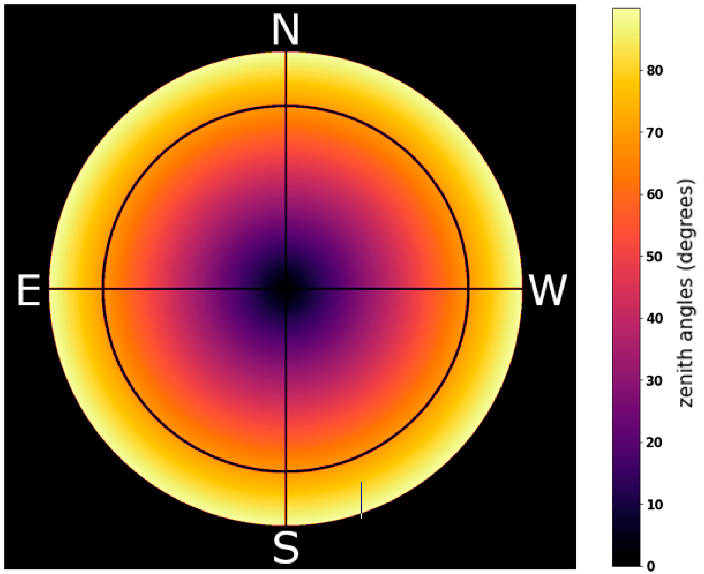
2.1. Signal Preprocessing

The machine learning task needs a well-defined characterization of the signal used as input in the model to be trained. Here, we proposed a method that uses the principal plane radiance as input signal. This choice relies on the dependency between radiance along the principal plane of the sun and the aerosol optical parameters [40,41]. This signal is mainly sensitive to the amount of aerosol and the particle size, which can be taken into account by AOD and AE, respectively. In that sense, our method is based on the method implemented by Cazorla et al. [25]. However, they used a representative single value of the principal plane radiance together with the solar zenith angle as inputs for a neural network model. In contrast, we performed a different selection of signals using the whole principal plane signal to assure a robust extraction of the main features associated with aerosols. To work with a clean, smoothed and aerosol-representative signal, we then follow a three-step process: (A) crop-off the images, (B) partial cloud screening and (C) generation of input signals.

(A)

Crop-off the images:

First, we crop-off each image to use only the viewing zenith angles less than 70° (the black inner circle in Figure 1). This allows us to avoid the presence of the surrounding buildings and other instruments deployed in BASS for larger observation angles close to the horizon. In addition, a cloud-free sky presents a radiative symmetry with respect to the principal plane. Therefore, the image is rotated so that the principal plane is a vertical line with the Sun in the south (the bottom part of the image in Figure 1). Then, we define an angular sector with the Sun as a vertex and the principal plane (being the line crossing the center of the Sun and the center of the image) as the bisector. The width of the sector is proportional to the scattering angle values (Figure 2a) that varies from 14° to 76°. We have chosen this range of scattering angle because is the maximum range shared by all solar positions reached throughout the year. This solution allows the solar zenith angle of each image to be examined independently. The minimum scattering angle (14°) has been chosen to avoid the saturated area in the circumsolar region, especially in the presence of a large aerosol load [31]. From now on, the defined angular sector will be our working area within the image. Thus, only this region is important to our cloud screening and the rest of the image can be partially or totally cloudy, with no effect on our input signal generation. This is a real advantage of our method for the selection of images in the available dataset, as specified in the next part (B).

(B)

Partial cloud screening:

For our analysis, we have used only images taken in well-defined sky conditions; namely, the part of the image defined as the working area in Section 2.1 (A) should be cloudless. To identify and select images fulfilling the cloudless condition, we used a symmetry criterion only applied within the selected working area of the images. In particular, we have used a parameter (γ_sim) based on the mirror symmetry along the principal plane of each channel. Below, we detail the procedure to obtain this and the other parameter needed in order to obtain the final Equations (1)–(4). Isolines of scattering angles within the selected angular sector (in the range 14°–76°, in steps of 2°) have been chosen and split in two branches (+; −), symmetrically to the principal plane. Then, the radiance (L_i⁺, L_i⁻) of each branch is subtracted pixel by pixel in absolute value and summed up for all the pixel-pairs (k) within each isoline of scattering angle (j) (Equation (1)). Subindex i accounts for the camera channels (i = R, G, B). Then, the sum of these differences is normalized to the averaged radiance in the portion of isoline ($\overline{L\left(i,j\right)}$). Finally, γ_sim is obtained as the average over all the isolines (Equation (2)). γ_sim takes low values for symmetric images. Overcast conditions share with totally clear-sky a high degree of symmetry and similar values of γ_sim. To differentiate both sky situations, we use an additional parameter (γ_brr) based on the blue-to-red ratio (BRR) within the angular sector under consideration. This has been evaluated firstly by calculating the BRR on each isoline, as the ratio of blue (L_B) and red (L_R) radiances (Equation (3)), and then averaging on the isoline itself. Finally, we derive γ_brr as the average over all the isolines (Equation (4)). In Equations (3) and (4), the indexes, i, j, k have the same meaning as in Equations (1) and (2).

$$\gamma \left(i,j\right)=\frac{{\sum }_{k=1}^{\frac{1}{2}{N}_j}{\left|L_i^{+}-L_i^{-}\right|}_k}{\overline{L\left(i,j\right)}}$$

(1)

$${\gamma }_{sim}\left(i\right)=\frac{{\sum }_{j=1}^M\gamma \left(i,j\right)}{M}$$

(2)

$${\gamma }_{brr}\left(j\right)=\frac{{\sum }_{k=1}^{N_j}\frac{L_B\left(k\right)}{L_R\left(k\right)}}{N_j}$$

(3)

$${\gamma }_{brr}=\frac{{\sum }_{j=1}^M{\gamma }_{brr}\left(j\right)}{M}$$

(4)

A partial clear-sky criterion can be derived from the histograms of the parameters γ_sim and γ_brr obtained from all the images in our dataset (Figure 2). The black vertical lines in the two histograms represent the clear sky threshold for the dataset: the images with high symmetry, within the part of the image considered, lie on the left of the black line (Figure 3a). This criterion allows clouds that are outside of our working area. This threshold has been chosen by dividing the histogram of the green channel (i = 2) symmetry parameter between its characteristic peak and its skewed part. On average, clear images have the blue component much stronger than the red one, unlike complete overcast condition cases. Therefore, images that fulfill the γ_sim criterion lie on the right of the black line in the histogram of γ_brr (Figure 2b). The presence of a bimodal distribution indicates a clear separation between cloud and cloud-free modes [40]. Cloud-free images within our working area correspond to values of γ_sim lower than 0.033 and γ_brr greater than 1.3 (right mode in Figure 2b). Our criterion, applied only in the region of interest within the images, allows us to have about 90,000 available images, which are 25,000 more than if the clear-sky criterion were applied to the whole image. This is because our criterion allow the presence of clouds in the image but outside the region of interest for constructing our signal. This presents a clear advantage in terms of the amount of available data, not only for building and testing our ML models but also for the number of images on which our models can be applied operationally. To note, we chose the green channel frequencies of γ_sim to determine the threshold of symmetric sectors because of the trade-off between the low sensitiveness of the blue channel to cloud presence and the high sensitiveness of red channel that decreases sensibly the number of symmetric sectors and available images. For this reason, we call this process ‘partial’ and delegate to a second step of analysis for the possibility of cleaning unwanted results (Section 3.2). Choosing images fulfilling both criterion may also imply limitations in the AOD used in our study, since most of the largest AOD values may be difficult to differentiate from clouds (zone between the two peaks). However, with these thresholds, we avoid most of the cloud contamination within our working area, and, finally, in our signal. In addition, we obtain a compromise between the number of images and the ranges of AOD and AE to be used in our ML model, which are around, 0–0.6 for AOD and 0.20–2.30 for AE.

(C)

Generation of input signals:

Once the ‘clear-sky’ images were selected, we built our smoothed signal of the principal plane from a single image in the following way: we chose the isolines of the scattering angle in the range 14°–76° with 2° steps within our working angular section (Figure 3a). The solar zenith angle is limited to 75° to assure that the first scattering angle (14°) is available in all images. Finally, we obtain a principal plane-like signal by averaging the radiance throughout each isoline of scattering angle (Figure 2c). In this way, we derive a smoothed signal compared to the noise obtained directly from the principal plane measurements (Figure 3c). Figure 3c also shows another natural choice for the principal plane-like signal. In this case we work with the whole image. Therefore, for each considered scattering angle, the signal is averaged over its whole isoline (Figure 3b). The partial clear-sky criterion were applied to the whole image and thus is referred to as a completely clear sky condition. This method of retrieving a signal from the camera was previously tested for ML prediction and, unfortunately, it has not achieved the best results [42]. This is probably because the reproduction of a principal plane signal is very poor (Figure 3c) and consequently contains very low information related to aerosols. In fact, the isolines of scattering angle deviate from the symmetry observed for the radiance with respect to the principal plane. These deviations are more significant farther from the principal plane and especially within the solar aureole (low scattering angles) (Figure 3b). Therefore, the resulting signal shows also a high degree of variability as is indicated by the standard deviation associated with each scattering angle average (see the error bars in Figure 3c). Our method to extract the principal plane signal does not show any significant changes in radiance while focusing on our specified working area. As expected from the radiance symmetry close to the principal plane, our averaged signal closely replicates the principal plane radiance, reducing the noise by smoothing. In addition, the standard deviation of the signal throughout the isoline section is relatively low. It increases only for scattering angles in which our camera optics produce sharpened peaks (brightness points) along the principal plane (Figure 3c). This represents a stronger property of radiative symmetry around the principal plane: the values of calibrated radiance do not change appreciably in a section of an isoline close and symmetric with respect to the principal plane. These characteristics allow us to fully trust in our clear and smoothed signal that preserve all the aerosol features (Figure 4) necessary to be used as input for ML. In Figure 4, we can also appreciate the different behavior of the principal plane proxy developed in this section when changing aerosol scenarios. In both cases, the radiance and its slope in the proximity of the Sun aureole are the most indistinctive and varying features associated with AOD and AE changes. This sort of degeneration with AOD and AE is expected to be dealt with by our ML models.

In Figure 4 we reproduce the smoothed principal plane signals obtained in sampled cases of fixed AOD and varying AEs (a) and fixed AE and varying AODs (b). The differences in signals are evident and the ML method has to model these differences into well-separated predictions in case of a totally clear sky condition. Unfortunately, this is not a scenario permitted by our partial clear-sky criterion and therefore justifies the posteriori research of a method that at least separates, with an independent criterion, well-predicted data from the other predictions. The method proposed in this paper will be discussed in Section 3.2.

Finally, we explicitly point out that the smoothing process of radiances in the principal plane arise from the necessity of dealing with strong spots of light due to glitters on it (Figure 3c). Since only the pure principal plane signal is related to the aerosol properties that we want to predict, our aim is to reproduce the pure principal plane signal with the help of this smoothing. This is a satisfactory reason to proceed in this way, although it is certainly not the only reason.

2.2. Machine Learning Model: Gaussian Process Regression

We have chosen a Gaussian process (GP) with a Matern kernel of 3/2 as machine learning model for the regression task. A GP is, by definition, a collection (potentially infinite) of random variables such that the joint distribution of every finite subset of random variables is multivariate Gaussian. Following Rasmussen and Williams [43], we describe how to derive the probabilistic way of this approach to obtain future predictions. The starting point for the theory of GP is the Bayesian analysis of a standard linear regression. Although the Bayesian linear regression works in the weight space instead of the GP functions space, it will be demonstrated that the treatment is equivalent or, better than GP, including the Bayesian linear regression case. Thus, we start with a linear model with some Gaussian noise.

$$f\left(x\right)=x^{T}w, y=f\left(x\right)+ϵ$$

(5)

where w is the linear weight, x the input variables and ε is the Gaussian noise with normal distribution $ϵ ~ N \left(0,{\sigma }_n^2\right)$. In the Bayesian scenario, the likelihood distribution is important in deriving the posteriori distribution, so we find it in this case with the aid of the independent Gaussian noise:

$$p\left(y:X,w\right)={\prod }_{i=1}^{n}p\left(y_i:x_i,w\right)=\frac{1}{{\left(2\pi {\sigma }_n^2\right)}^{\frac{n}{2}}}\exp \left(-\frac{{\left|y-X^{T}w\right|}^2}{2{\sigma }_n^2}\right)=N\left(X^{T}w, {\sigma }_n^{2}I\right)$$

(6)

An a priori distribution for the parameters should also be discussed: we put for them a zero mean Gaussian priori with covariance matrix ${\mathsf{\Sigma }}_p$ or equivalently $w ~ N \left(0,{\mathsf{\Sigma }}_p\right)$. Therefore, final inference in the Bayesian linear model is based on the posteriori formula of Bayes:

$$p\left(w:y,X\right)=\frac{p\left(y:X,w\right)p\left(w\right)}{p\left(y:X\right)}$$

(7)

In writing in the formula only the terms containing the weights and then making the calculations, we obtain:

$$p\left(w:y,X\right) ~ N\left(\frac{A^{-1}Xy}{{\sigma }_n^2}, A^{-1}\right)$$

(8)

where $A={\sigma }_n^{-2}X{X}^T+{\mathsf{\Sigma }}_p^{-1}$. In the Bayesian way to predict a test case, it is common to average over all possible parameter’s values weighted by the posteriori probability calculated:

$$p\left(f_{*}:x_{*},X,y\right)={\int }^{ }p\left(f_{*}:x_{*},w\right)p\left(w:X,y\right)dw=N\left(\frac{x_{*}^T{A}^{-1}Xy}{{\sigma }_n^2},x_{*}^T A^{-1}{x}_{*}\right)$$

(9)

The predictive distribution is again Gaussian with mean given by the posteriori mean of weights multiplied by the test input. To overcome the limitation of linear regression, the simplest choice is that of projecting the inputs into some high dimensional space and then performing the linear regression in this space rather than in the input space itself. This is similar to the more famous supporting vector machine classifier in the case of no linear regression models. The model is still linear in parameters so is analytically tractable. Now we have:

$$f\left(x\right)=\varphi {\left(x\right)}^{T}w$$

(10)

with N as the dimension of parameters and ϕ as the mapping of input in higher dimensional space. The analysis of this case is analogous to the previous one, so we have:

$$\begin{array}{c}{f}_{*}:x_{*},X,y ~ N\left(\frac{\varphi {\left(x_{*}\right)}^T{A}^{-1}\varphi y}{{\sigma }_n^2},\varphi {\left(x_{*}\right)}^T A^{-1}\varphi \left(x_{*}\right)\right)=\hfill \\ \hspace{1em}N\left(\frac{\varphi {\left(x_{*}\right)}^T{\Sigma }_p\varphi \left(x\right){\left(K+{\sigma }_n^2\right)}^{-1}y}{{\sigma }_n^2},\varphi {\left(x_{*}\right)}^T {\Sigma }_p\varphi \left(x_{*}\right)-\varphi {\left(x_{*}\right)}^T{\Sigma }_p{\left(K+{\sigma }_n^2\right)}^{-1}\varphi {\left(x\right)}^T{\Sigma }_p\varphi \left(x_{*}\right)\right) \hfill \end{array}$$

(11)

with $\varphi =\varphi \left(x\right)$, $A={\sigma }_n^{-2}\varphi {\varphi }^T+{\mathsf{\Sigma }}_p^{-1}, K=\varphi {\left(x\right)}^T{\mathsf{\Sigma }}_p\varphi \left(x\right)$ and $f_{*}, x_{*}$ being the prediction and the features of the test data. Now, we define $K\left(x,x^{\prime }\right)=\varphi {\left(x\right)}^T{\mathsf{\Sigma }}_p\varphi \left(x^{\prime }\right)$ which is the covariance function or kernel. If the algorithm is defined in terms of inner product in the input space like the ones in the previous formulas, one can easily replace these inner products with the kernel in the higher dimensional space: this is the kernel trick, so the kernel thus becomes most important than knowing the feature space.

We now specify the Gaussian process by the mean and the covariance of the function of the ensemble:

$$m\left(x\right)=E\left[f\left(x\right)\right], k\left(x,x^{\prime }\right)=E\left[\left(f\left(x\right)-m\left(x\right)\right)\left(f\left(x^{\prime }\right)-m\left(x^{\prime }\right)\right)\right]$$

(12)

and calling the process itself:

$$f\left(x\right) ~ GP\left(m\left(x\right),k\left(x,x^{\prime }\right)\right)$$

(13)

In this functional case, the variables are the values of the function f at location x. In general, and in the case of this study, we take the mean values to be zero. We now show that an example of the Gaussian process is the Bayesian linear regression in the feature space: Thus f(x) and f(x′) are jointly Gaussian with zero mean and covariance given by the kernel. In the present study, we choose for the kernel, the Matern 3/2 with the formula:

$$K\left(x,x^{\prime }\right)={\sigma }^2\left(1+\frac{\sqrt{3}d}{\rho }\right)\exp \left(-\frac{\sqrt{3}d}{\rho }\right)$$

(14)

where d is distance between points and the σ, ρ positive parameters of the kernel that are learned in the training. The predictive final equation for the Gaussian process regression is given by the covariance correction by the Gaussian noise error as in the case of the Bayesian linear model explained before:

$$cov\left(y\right)=K\left(X,X\right)+{\sigma }_n^{2}I$$

(15)

Thus, we can write the joint distribution of observed target values and the function values at the test location:

$$\left(\begin{array}{c}y\\ f_{*}\end{array}\right) ~ N\left(0, \left[\begin{array}{cc}K\left(X,X\right)+{\sigma }_n^{2}I& K\left(X,X_{*}\right)\\ K\left(X_{*},X\right)& K\left(X_{*},X_{*}\right)\end{array}\right]\right)$$

(16)

where $K\left(X,X_{*}\right)$ denotes the $n\times n_{*}$ matrix covariance calculated for all pairs of training and test points and ${\sigma }_n^2$ denotes the variance of error noise. The key predictive equation derives from this priori as:

$$f_{*}:X,y,X_{*} ~ N\left(\overline{f_{*}}, cov\left(f_{*}\right)\right)$$

(17)

where: $\overline{f_{*}}=E\left[f_{*}:X,y,X_{*}\right]=K\left(X_{*},X\right){\left[K\left(X,X\right)+{\sigma }_n^{2}I\right]}^{-1}y$

$$cov\left(f_{*}\right)=K\left(X_{*},X_{*}\right)-K\left(X_{*},X\right){\left[K\left(X,X\right)+{\sigma }_n^{2}I\right]}^{-1}K\left(X,X_{*}\right)$$

(18)

This last formula allows the distribution to make a prediction on unseen data based on test features and the training of the model. Among the advantages of the GP, we must point out that the model predictions are interpolated from the observations, making it a very good choice for the present study where the relation between the signals and the aerosol properties has been proven. Furthermore, the prediction is probabilistic so that one can compute empirical intervals of confidence and decide on them if it is necessary to calculate a new fit in a region of interest prone to low representation of points or overfitting. A good reason to choose the GP as an algorithm of regression in our prediction task can be justified by the fact that the general random noise expected from remote sensing retrievals shows a Gaussian behavior, which is the same assumption and theory that stands behind flexible models used for generalized inversion retrievals of remote sensing aerosol measurements both for ground-based and satellite-based aerosols [44,45,46].

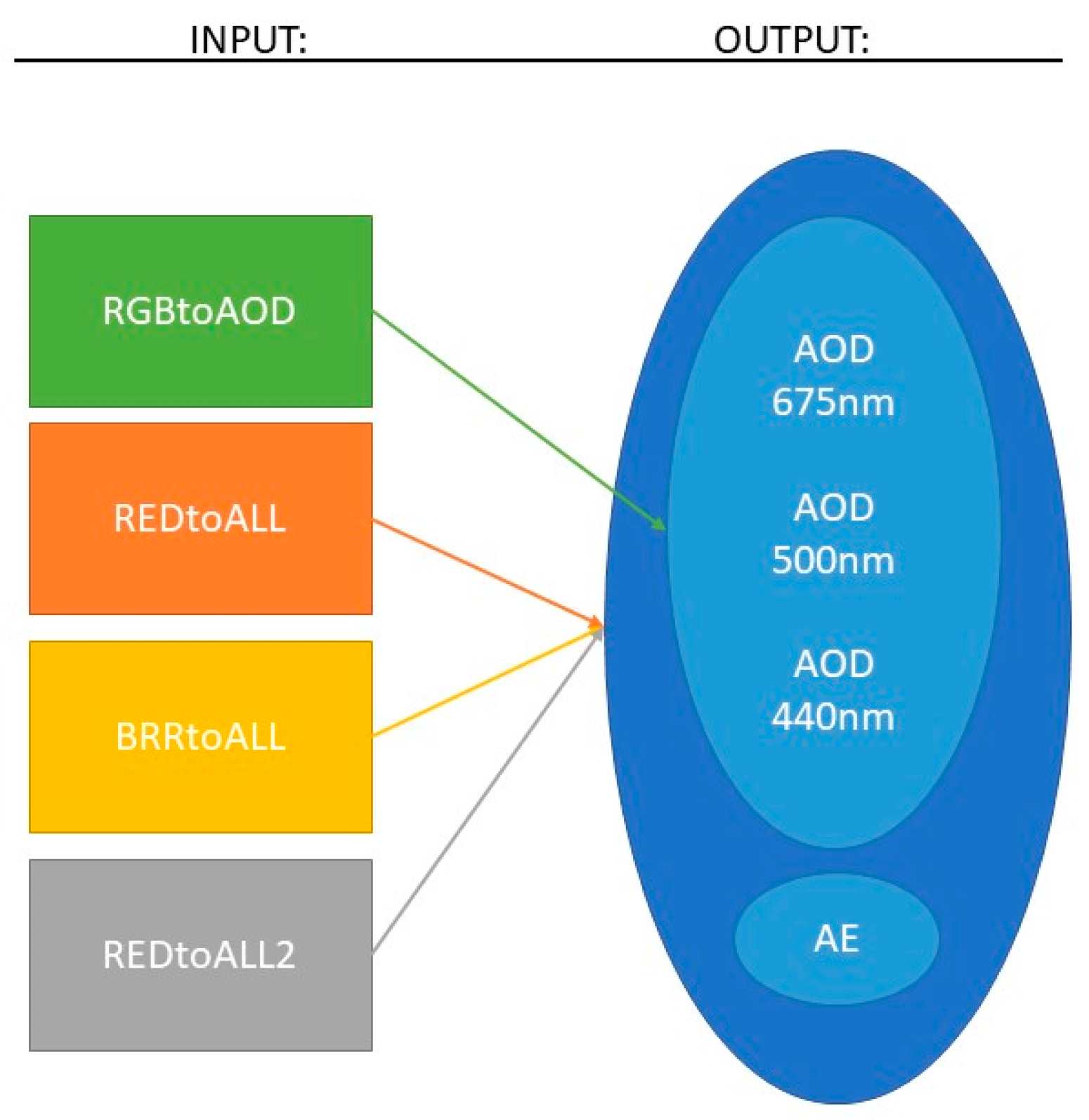
2.3. Approaches to Prediction

Four different approaches have been chosen to perform the prediction of AOD and AE (Figure 5). For the first approach, RGBtoAOD, signals from the RGB channels are individually related to AOD measured at its closest AERONET wavelength. Therefore, the principal plane-like radiance signal from the red, green and blue channels of the all-sky camera are related with the AOD measured by Cimel at 675, 500 and 440 nm wavelengths, respectively. This way, we have three ML models (one for each channel) with which only AOD predictions are possible. Secondly, for REDtoALL, only the red signals have been related to all the four outputs (three wavelengths of AOD and AE) using an equivalent number of models. In the third case, for BRRtoALL, a blue-red-ratio (BRR) signal has been built as the ratio between the blue and the red signals, and it is related to all the outputs in the four models (three wavelengths of AOD and AE). Finally, for REDtoALL2, a red signal again has been chosen to be the only input for just one multioutput model producing the four outputs simultaneously. In the four cases, a division into training and testing datasets from the complete dataset must be performed. The choice of the elements of both datasets is made in a random way, using two-thirds of the complete dataset for the training dataset and the remaining third for the validation of our models (test set). The complete dataset consist of 32,000 images, of which N = 14,000 of them are for the train dataset while the testing dataset uses N’ = 18,000 samples, according to the conditions detailed in Section 2.1. Generally speaking, one should select a fraction of the total dataset to create a test dataset from a maximum a third of it. However, in the present scenario, we would like to replicate a simulated forecasting approach that predicts aerosol features on a large number of test images and relegate to the training dataset only the number of images that allows the model to be created in a reasonable time (almost 15,000 images) without appreciable changes in terms of statistical results (verified but not showed here). We finally chose four approaches for prediction in order to better appreciate if all the channel signals are needed to predict aerosol properties at similar wavelengths or if just one channel signal (or BRR one) is sufficient for achieving good statistical results.

To assess the prediction performance of each model, we perform a regression analysis between our results and AERONET test dataset. In addition, we use different parameters in the validation analysis. The first parameter is the percentage of predictions that fall aside from AERONET measurements within its typical uncertainty, namely 0.01–0.02 for AODs and 0.1–0.2 for AE. Secondly, we use the root mean square error (RMSE) and mean absolute error (MAE) to estimate how globally close the predictions are with respect to AERONET measured values together with its correlation coefficient R². In the following, we report the formula of the metric used in the statistical evaluation of the prediction:

$$MAE=\frac{{\sum }_{i=1}^N\left|pre{d}_i-mea{s}_i\right|}{N}$$

(19)

$$RMSE=\sqrt{\frac{{\sum }_{i=1}^N{(pre{d}_i-mea{s}_i)}^2 }{N}}$$

(20)

$$R^2=1-\frac{{\sum }_1^N{\left(pre{d}_i-mea{s}_i\right)}^2}{{\sum }_1^N{\left(pre{d}_i-\overline{pred}\right)}^2}$$

(21)

3. Results

3.1. The Raw Prediction Performances

To evaluate the performance of the described models in predicting spectral AOD and AE, we carried out several tests of different single session predictions. Each of them varies among the others in the chosen data for testing and training datasets. The data for all these sessions are selected randomly following the characteristics described in Section 3.2. In comparing the results provided by these sessions with AERONET data, we conclude that no significant differences are shared between different sessions. Consequently, we decided to analyze one of them as a representative of all. Thus,

Table 1. Statistical evaluation of the performance of the single session prediction of our proposed methodology. Nu is the percentage of results within the AERONET uncertainties: 0.01–0.02 for AOD and 0.01–0.2 for AE. Results for the data quality assured selection (QA) are also reported. * Percent of predictions that fall close to AERONET values within the AERONET uncertainties (0.01–0.02 for AOD and 0.1–0.2 for AE).

Methods	Outputs	Nu * (%) (QA)	MAE (QA)	RMSE (QA)	a (QA) ± δ	b (QA) ± δ	R2 (QA)	PERC QA (%)
RGBtoAOD	AOD675	81–93 (95–99)	0.006 (0.004)	0.012 (0.005)	0.904 (0.992) ± 0.002	0.0066 (0.0005) ± 0.0001	0.96 (0.99)	70
	AOD500	73–85 (87–96)	0.010 (0.005)	0.019 (0.01)	0.883 (0.989) ± 0.002	0.0118 (0.0011) ± 0.0002	0.94 (0.99)	75
	AOD440	60–75 (73–87)	0.016 (0.004)	0.030 (0.027)	0.851 (0.951) ± 0.003	0.024 (0.006) ± 0.0004	0.88 (0.97)	74
REDtoALL	AOD675	81–93 (95–99)	0.006 (0.004)	0.012 (0.005)	0.904 (0.992) ± 0.002	0.0066 (0.0005) ± 0.0001	0.96 (0.99)	70
	AOD500	74–88 (91–98)	0.008 (0.004)	0.015 (0.008)	0.913 (0.991) ± 0.002	0.0095 (0.0009) ± 0.0002	0.96 (0.99)	68
	AOD440	70–85 (88–97)	0.010 (0.003)	0.017 (0.01)	0.914 (0.988) ± 0.002	0.0111 (0.0012) ± 0.0002	0.96 (0.99)	67
	AE	64–81 (87–96)	0.12 (0.05)	0.18 (0.09)	0.746 (0.968) ± 0.003	0.342 (0.041) ± 0.004	0.78 (0.97)	52
BRRtoALL	AOD675	77–87 (81–90)	0.008 (0.004)	0.014 (0.012)	1.009 (1.012) ± 0.002	0.0044 (0.0018) ± 0.0002	0.95 (0.97)	68
	AOD500	68–81 (73–84)	0.012 (0.005)	0.022 (0.022)	0.977 (0.993) ± 0.002	0.0099 (0.0068) ± 0.0003	0.92 (0.93)	68
	AOD440	63–78 (68–82)	0.015 (0.005)	0.028 (0.028)	0.962 (0.983) ± 0.003	0.0136 (0.0097) ± 0.0004	0.91 (0.92)	68
	AE	70–85 (86–97)	0.10 (0.05)	0.16 (0.08)	0.874 (0.981) ± 0.004	0.178 (0.026) ± 0.003	0.83 (0.98)	58
REDtoALL2	AOD675	81–93 (95–99)	0.006 (0.004)	0.012 (0.005)	0.904 (0.992) ± 0.002	0.0066 (0.0005) ± 0.0001	0.96 (0.99)	70
	AOD500	74–88 (91–98)	0.008 (0.004)	0.015 (0.008)	0.913 (0.991) ± 0.002	0.0095 (0.0009) ± 0.0002	0.96 (0.99)	68
	AOD440	70–85 (88–97)	0.010 (0.003)	0.017 (0.01)	0.914 (0.988) ± 0.002	0.0111 (0.0012) ± 0.0002	0.96 (0.99)	67
	AE	64–81 (87–96)	0.12 (0.05)	0.18 (0.09)	0.746 (0.968) ± 0.003	0.342 (0.041) ± 0.004	0.78 (0.97)	52

shows a summary of some of the statistical parameters used to evaluate the performance of our ML models in comparison with AERONET measurements. In general, our ML results for the four methods display a good accordance with AERONET measurements for AOD and AE. R² is higher than 0.88 for AOD predictions while the RMSE values are below 0.03 and 0.18 for AOD and AE, respectively. In the worst case, the 60% and 64% of the predictions of AOD and AE fall within the AERONET typical uncertainties of 0.01 and 0.1 with 75% and 81% within 0.02 and 0.2, respectively. In the best case, we reached 81% for the 675 nm AOD prediction and 70% for the AE prediction. In general, the slopes are higher than 0.96 and 0.92 for AOD and AE, respectively. In terms of the best AOD overall prediction, the REDtoALL method shows the best performance regarding the percentage of the predicted AOD within the AERONET uncertainty, with more than 81% below 0.01, which is comparable with the results of the RGBtoAOD method. We appreciate that the BRRtoALL method shows a slightly better performance on the higher values of AOD (Figure 6), which shows less outliers and tends to underestimate the measurements as in the REDtoALL case in Figure 6a. This behavior was seen in all the different predictions involving the two methods, indicating that the better performance was the BRRtoALL method in characterizing a high AOD range.

For the AE, the best results were obtained from the approach BRRtoALL, with 70% of the predictions within the AERONET uncertainty. This was expected since it accounts for the information of the blue and red channels, which are closest to the AERONET wavelengths used for the AE calculation. The use of the red signal only (REDtoALL and REDtoALL2) to predict the AE displayed good performance also, with 64% of predictions within the uncertainty of AERONET retrieval. Worth mentioning, although not shown here, is that a trial, which we performed, of generating the AE from predicted AODs has been attempted, showing similar results (within uncertainties) with respect to those provided by the ML method BRRtoALL.

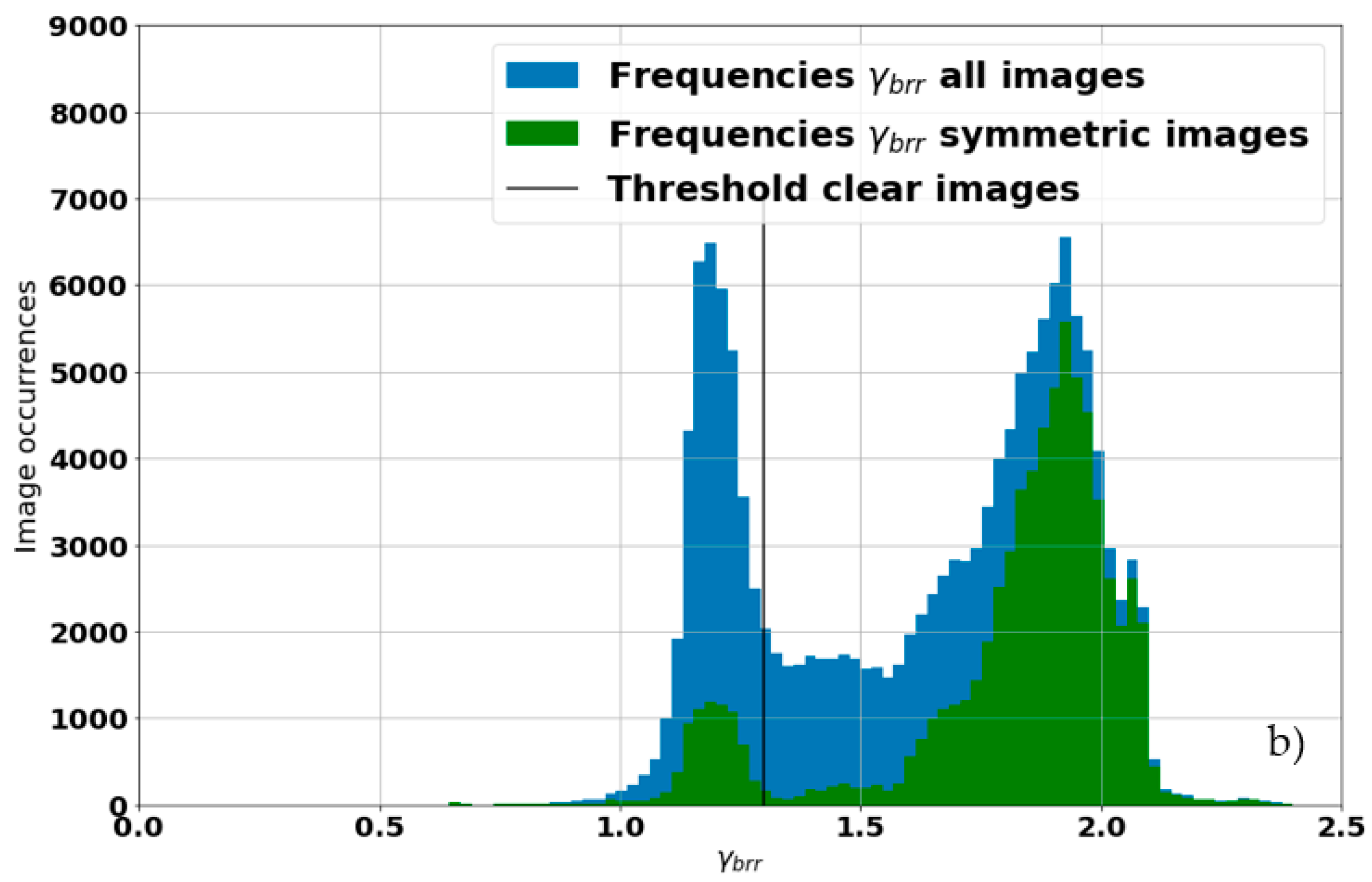
3.2. Data Quality Control

In the previous section, we have shown how the simple predictions are good but not good enough to justify a use of the camera, and this methodology, as a routine instrument for retrieving aerosol properties. This is due to the weak condition that we called partial cloud screening: the presence of not completely clear images in the test dataset and, most importantly, in the train dataset makes the prediction less accurate. Fortunately, the GP regression method returns with the predictions and also the standard deviations associated with them for the model. From this important feature of the model, we can develop an a posteriori criterion that overcomes the problems of the general method associated with the presence of clouds. This feature is also very useful where the ML method constitutes an indirect measurement, as in our approach, in which it is applied to direct measurements of radiances from an all-sky camera. We call this approach data quality control and we call predictions that pass the criterion data quality assured. Therefore, we derive a quality check of the predictions based on the standard deviation: this criterion is based on the fact that if we select the ‘good’ predictions as the ones with a standard deviation less than a fixed threshold, the overall performance of the prediction increases. Figure 7 shows a sensitivity analysis of how the percentage of the prediction within the AERONET uncertainties and the percentage of quality assured images grows with increasing thresholds of the standard deviations. This is true for all the four methods used and all the AOD or AE predictions.

Since no definite criterion can be extracted from these graphs, we proposed a statistical one. Thus, for every session of prediction, we evaluate the RMSE of this difference and applied it as a threshold for the standard deviations. With this approach, we obtained the results in Table 1 labeled as QA, and the scatterplots of the predictions associated with the quality assured selection which are in the right columns of Figure 6. At a cost of almost 30% of images rejected, we finally obtained excellent performances from the four methods. In particular, the REDtoALL method and the fastest REDtoALL2 method showed great performances that can be appreciated in the percentage of predictions within the AERONET uncertainties and the other performance evaluators. On the other hand, the difficult challenge of retrieving the AE was also successful but at the cost of 50% of rejected images in all the methods. We can associate with each prediction session an uncertainty value given by 0.02 for AOD and 0.2 for AE; in this way, almost 90% of predictions lied in the corresponding AERONET uncertainties.

3.3. Comparison with Other Machine Learning Models

The final results explore the power of our model compared with other more classical machine learning methods. Here, we will consider two of them: an artificial neural network (ANN) and a random forest (RF). The comparison of the prediction is shown in

Table 2. Statistical evaluation of the comparison between the prediction of our proposed methodology and the predictions of an ANN and a RF. * Percent of predictions that fall close to AERONET values within the AERONET uncertainties (0.01–0.02 for AOD and 0.1–0.2 for AE).

Models	Outputs	Nu * (%) (QA)	MAE (QA)	RMSE (QA)	a (QA) ± δ	b (QA) ± δ	R2 (QA)	PERC QA (%)
GP (Red to all)	AOD675	81–93 (95–99)	0.006 (0.004)	0.012 (0.005)	0.904 (0.992) ± 0.002	0.0066 (0.0005) ± 0.0001	0.96 (0.99)	70
	AOD500	74–88 (91–98)	0.008 (0.004)	0.015 (0.008)	0.913 (0.991) ± 0.002	0.0095 (0.0009) ± 0.0002	0.96 (0.99)	68
	AOD440	70–85 (88–97)	0.010 (0.003)	0.017 (0.01)	0.914 (0.988) ± 0.002	0.0111 (0.0012) ± 0.0002	0.96 (0.99)	67
	AE	64–81 (87–96)	0.12 (0.05)	0.18 (0.09)	0.746 (0.968) ± 0.003	0.342 (0.041) ± 0.004	0.78 (0.97)	52
ANN (Red to all)	AOD675	75–90	0.009	0.015	0.904 ± 0.004	0.0066 ± 0.0002	0.93
	AOD500	58–84	0.011	0.018	0.901 ± 0.001	0.0111 ± 0.0001	0.94
	AOD440	56–80	0.013	0.019	0.920 ± 0.003	0.0080 ± 0.0004	0.95
	AE	39–68	0.17	0.24	0.669 ± 0.008	0.43 ± 0.02	0.67
RF (Red to all)	AOD675	81–93	0.007	0.013	0.903 ± 0.003	0.0059 ± 0.0001	0.95
	AOD500	69–87	0.010	0.016	0.913 ± 0.003	0.0074 ± 0.0004	0.96
	AOD440	61–83	0.012	0.019	0.908 ± 0.003	0.0091 ± 0.0007	0.95
	AE	48–72	0.16	0.22	0.669 ± 0.008	0.43 ± 0.02	0.67

, where, along with the same metrics reported for the Gaussian process case, the same results of Table 1 have been reported to better highlight the comparison. For the three models reported in Table 2, the results concern only the case we named REDtoALL in the rest of the paper: only the method with the best result has been used for all the model comparisons.

From Table 2, we can appreciate that the ANN and the RF models are even worse than the GP model in the absence of the data quality selection. The only statistical metric that is comparable and performs better in some cases is the linear fit between the predicted and the actual data. However, the most important models had percentages of points predicted close enough to the actual data: MAE, RMSE and R² all perform worse for the ANN and the RF compared with our methodology. In some ways, this is not surprising because these models are ‘data-eaters’ and need more training data to show the best performances. On the other hand, a Gaussian process regressor can perform satisfactorily and even in a reasonable computing time with a number of training observations around the order of 10,000. This is a clear advantage in the present remote sensing case. Indeed, in our one and a half years of measurements, we were able to build a dataset for machine learning purposes that can be well suited for our methodology involving a Gaussian process regressor. Furthermore, with the new incoming data, the model can be readily used as a forecasting methodology, whereas in the case of ANN and RF, other data and scenarios are necessary to train those models.

4. Discussion

The excellent results obtained in our quality assured predictions mostly relied on the ability of the approach we used to build the input signal and select the proper well-predicted aerosol features, which is one of the novelties of our method. Working just within the region of the image containing the principal plane has several advantages in terms of the quality of the input signal and the number of images available to apply our methodology. Therefore, we obtain a clean and smoothed signal in the principal plane that avoids cloud contamination and is representative of the aerosol features, which is mainly sensitive to the aerosol load and size (through AOD and AE, respectively). Moreover, we can also use partially cloudy images since it is enough to have clear sky in our region of interest around the principal plane. Whatever the method used, our approach showed numerical stability in the prediction, no matter the training dataset involved in building the ML model. Furthermore, choosing a hybrid approach provides great flexibility to take advantage of all the best features of the methods. For example, if images within a range of AOD or AE are poorly represented in the dataset, the choice should be the BRRtoALL method, since it seems to have predicted better in this situation. Otherwise, if the set of available images for a site is related to a large range of AOD and AE values with enough representativeness, the choice should be the REDtoALL methods to retrieve the AOD and, for example, to choose the one that predicts all the properties at once to spend less computing time.

Usually, ML models perform better the better they are trained or as much as the target closely resembles the training data. In addition, the greatest virtue of the ML models lies in its ability to learn situations not seen in the training data if the casuistry of the training data is wide. However, they can be sensitive to different issues related to the quality, number and casuistry of the training data; intrinsic differences between input and output data, whether of an instrumental nature, spatial-temporal coincidence, or other characteristics of the observations [43]. In our case, we have analyzed some of these issues to confirm the robustness of our models, our results and ultimately the potential and scope of our predictions.

Most of the instrumental differences between Cimel and SONA (e.g., the FOV of camera single pixel, central peak wavelength and bandwidth of the RGB filters) should be managed by the ML techniques in finding the final relationship between inputs and outputs of the models. Therefore, we do not expect significant deviations in the validation of our results due to those instrumental differences. Conversely, the time shift (4 min) between the two measurements may be a non-negligible issue resulting in an intrinsic source of final uncertainties [30,47]. Our model outputs did not show any significant differences (less than 1%) when the temporal tolerance between AERONET and SONA coincident measurements varied from 1, 2, 4, 5 to 15 min. This indicates that the 4 min tolerance initially used for the temporal coincidence in relating all-sky camera images and AERONET measurements may limit the associated uncertainties, since due to in cloud-free conditions, no significant variations are expected in the aerosol load or type (i.e., AOD and AE) in such a short time. Our results do not show any sensitivity to the solar zenith angle. In addition, negligible differences among the results are observed if the solar zenith angle is used or not as input in our models. This is what we expected since the principal plane radiance curve already has information about the solar position [24,25].

Our results agree with those obtained using AI techniques applied to remote sensing retrievals, either to ground-based or satellite-based measurements [15,16,19,25,26,27]. In general, satellite retrievals of AOD and AE improve the accuracy of the physically based methods when AI techniques are used. Correlation coefficients up to 0.99 result when comparing satellite-derived results against AERONET observations [15,16,19]. Moreover, better agreement is reported for AOD than for size-related parameters (e.g., AE), which agree with our observations. Our results significantly improve those results obtained previously using all-sky cameras, either through physical methods or AI approaches [25,32]. Cazorla et al. [25] used an ANN together with a representative point of the principal plane of the image and the solar zenith angle as inputs. They achieved good results for the AOD in terms of correlation coefficients, with a minimum R² value of 0.93 and a number of predictions within the AERONET uncertainties of 81% and 80% for AOD at 675 and 440, respectively. Their results were poorer for AE predictions with only 50% of their predictions within the AERONET uncertainties. In both cases, for AOD and AE, our predictions are more accurate in comparison with AERONET, with R² over 0.96 in all cases and higher percentages of the predicted quality assured values (Table 1). This is especially relevant for the prediction of AE in which our results represent a significant improvement. Apart from the method used (ANN vs. GPR), there are significant methodological differences between the approach followed by Cazorla and ours that can help to explain the different precision of both results. On the one hand, their conclusions rely on fewer data points. Even if the number of points were enough for a statistical conclusion, they represent about one thirtieth of the dataset used in this work, and lower numbers of points can severely affect the overfitting effect. Secondly, we worked with a higher quality input signal, since it is smoothed and cloud-screened even accounting for a posteriori check. In addition, we consider a large portion of the principal plane that clearly highlights the aerosol information.

In a recent study, Román et al. [32] used almost 17,000 sky-camera calibrated images and the GRASP algorithm [45] to retrieve the AOD at the effective wavelengths of the camera (605, 536 and 467 nm). GRASP inversions are physically constrained by surface reflectance and vertical profiles of aerosol size distribution. Their results compare well with AERONET with a slightly underestimation of the AOD in the high range. The reported correlation is significantly poorer than that seen in our comparisons, with an R² of 0.88.

5. Conclusions

Four methods for retrieving aerosol properties from a well-calibrated all-sky camera have been presented. These methods used a ML approach to relate AOD and AE from AERONET measurements, with different signals based on the radiance of the principal plane, measured by an all-sky camera. A quality assurance criterion of the output based on standard deviation propagated by the Gaussian process regression was also proposed, which sensibly improved the accuracy of our results. The overall uncertainties for the predictions assigned to our models were of ±0.02 for AOD and ±0.2 for AE following the data quality selection of the predictions. All of them exhibited excellent agreement with the AERONET values, with correlation coefficients greater than 0.92. In addition, the percentage of predicted values within the AERONET uncertainties was better than 88% for the output parameters of the best model.

These excellent results shown by our predictions mostly rely on the novel approach we used to build our input signal and the a posteriori data quality selection. Combined, it provides a clean, smoothed and cloud-screened signal that is able to highlight the aerosol features contained in the principal plane radiance. We found several advantages associated with our developed methodology, since it favors working with high quality input signals even when using partially cloudy scenes. In addition, this allows for increasing the number of available images for both building and applying our models.

Several tests have been carried out to evaluate the performance of our models. All of them displayed a high degree of numerical stability with no significant dependencies on the training dataset, instrumental or temporal differences between the input and output data, or solar zenith angle. These analyses support the robustness of our models, our results, and the potential and scope of our predictions. These excellent results from our quality assured criterion allows us to be confident in our models. Therefore, the excellent performance of our proposed methodology suggests that a well-calibrated all-sky camera can be routinely used to retrieve aerosol properties with sufficient accuracy. In conclusion, the operational performance of all-sky cameras can be significantly improved thanks to our work. All this is of great interest to atmospheric physics since it contributes to improving aerosol monitoring, both in global coverage and in the quality and accuracy of the measurements.

References

1. IPCC. Climate Change 2013: The Physical Science Basis. In Contribution of Working Group I to the Fifth Assessment Report of the Intergovernmental Panel on Climate Change; Stocker, T.F., Qin, D., Plattner, G.-K., Tignor, M., Allen, S.K., Boschung, J., Nauels, A., Xia, Y., Bex, V., Midgley, P.M., Eds.; Cambridge University Press: Cambridge, UK; New York, NY, USA, 2013; p. 1535. [Google Scholar]
2. Kim, D.; Ramanathan, V. Solar radiation budget and radiative forcing due to aerosols and clouds. J. Geophys. Res. Atmos. 2008, 113, 148–227. [Google Scholar] [CrossRef] [Green Version]
3. Eddy, C. Aerosol Direct Radiative Forcing: A Review. Atmos. Aerosols Reg. Charact. Chem. Phys. 2012, 379–394. [Google Scholar] [CrossRef] [Green Version]
4. Maciel, F.V.; Diao, M.; Patnaude, R. Examination of aerosol indirect effects during cirrus cloud evolution. Atmos. Chem. Phys. 2023, 23, 1103–1129. [Google Scholar] [CrossRef]
5. Manolache, C.; Boldeanu, M.; Talianu, C.; Cucu, H. Unsupervised deep learning models for aerosol layers segmentation. In Proceedings of the 2022 14th International Conference on Communications (COMM), Chongqing, China, 10–12 June 2022; pp. 1–6. [Google Scholar] [CrossRef]
6. Haywood, J.; Boucher, O. Estimates of the direct and indirect radiative forcing due to tropospheric aerosols: A review. Rev. Geophys. 2000, 38, 513–543. [Google Scholar] [CrossRef]
7. Lohmann, U.; Feichter, J. Global indirect aerosol effects: A review. Atmos. Meas. Tech. 2005, 5, 715–737. [Google Scholar] [CrossRef] [Green Version]
8. Pilahome, O.; Ninssawan, W.; Jankondee, Y.; Janjai, S.; Kumharn, W. Long-term variations and comparison of aerosol optical properties based on MODIS and ground-based data in Thailand. Atmos. Environ. 2022, 286, 119218. [Google Scholar] [CrossRef]
9. Luong, N.D.; Hieu, B.T.; Hiep, N.H. Contrasting seasonal pattern between ground-based PM2.5 and MODIS satellite-based aerosol optical depth (AOD) at an urban site in Hanoi, Vietnam. Environ. Sci. Pollut. Res. 2021, 29, 41971–41982. [Google Scholar] [CrossRef]
10. Yu, F.; Luo, G.; Nair, A.A.; Tsigaridis, K.; Bauer, S.E. Use of machine learning to reduce uncertainties in particle number concentration and aerosol indirect radiative forcing predicted by climate models. Geophys. Res. Lett. 2022, 49, e2022GL098551. [Google Scholar] [CrossRef]
11. Xie, W.; Liu, D.; Yang, M.; Chen, S.; Wang, B.; Wang, Z.; Xia, Y.; Liu, Y.; Wang, Y.; Zhang, C. SegCloud: A novel cloud image segmentation model using a deep convolutional neural network for ground-based all-sky-view camera observation. Atmos. Meas. Tech. 2020, 13, 1953–1961. [Google Scholar] [CrossRef] [Green Version]
12. Kolios, S.; Hatzianastassiou, N. Quantitative Aerosol Optical Depth Detection during Dust Outbreaks from Meteosat Imagery Using an Artificial Neural Network Model. Remote Sens. 2019, 11, 1022. [Google Scholar] [CrossRef] [Green Version]
13. Choi, W.; Lee, H.; Park, J. A First Approach to Aerosol Classification Using Space-Borne Measurement Data: Machine Learning-Based Algorithm and Evaluation. Remote Sens. 2021, 13, 609. [Google Scholar] [CrossRef]
14. Gong, X.; Wex, H.; Müller, T.; Henning, S.; Voigtländer, J.; Wiedensohler, A.; Stratmann, F. Understanding aerosol microphysical properties from 10 years of data collected at Cabo Verde based on an unsupervised machine learning classification. Atmos. Chem. Phys. 2022, 22, 5175–5194. [Google Scholar] [CrossRef]
15. Kang, Y.; Kim, M.; Kang, E.; Cho, D.; Im, J. Improved retrievals of aerosol optical depth and fine mode fraction from GOCI geostationary satellite data using machine learning over East Asia. ISPRS J. Photogramm. Remote Sens. 2021, 183, 253–268. [Google Scholar] [CrossRef]
16. Lipponen, A.; Reinvall, J.; Väisänen, A.; Taskinen, H.; Lähivaara, T.; Sogacheva, L.; Kolmonen, P.; Lehtinen, K.; Arola, A.; Kolehmainen, V. Deep-learning-based post-process correction of the aerosol parameters in the high-resolution Sentinel-3 Level-2 Synergy product. Atmos. Meas. Tech. 2022, 15, 895–914. [Google Scholar] [CrossRef]
17. Liang, T.; Liang, S.; Zou, L.; Sun, L.; Li, B.; Lin, H.; He, T.; Tian, F. Estimation of Aerosol Optical Depth at 30 m Resolution Using Landsat Imagery and Machine Learning. Remote Sens. 2022, 14, 1053. [Google Scholar] [CrossRef]
18. Lee, J.; Shi, Y.; Cai, C.; Ciren, P.; Wang, J.; Gangopadhyay, A.; Zhang, Z. Machine Learning Based Algorithms for Global Dust Aerosol Detection from Satellite Images: Inter-Comparisons and Evaluation. Remote Sens. 2021, 13, 456. [Google Scholar] [CrossRef]
19. Li, J.; Wong, M.S.; Lee, K.H.; Nichol, J.E.; Abbas, S.; Li, H.; Wang, J. A physical knowledge-based machine learning method for near-real-time dust aerosol properties retrieval from the Himawari-8 satellite data. Atmos. Environ. 2022, 280, 119098. [Google Scholar] [CrossRef]
20. Di Noia, A.; Hasekamp, O.P.; van Harten, G.; Rietjens, J.H.H.; Smit, J.M.; Snik, F.; Henzing, J.S.; de Boer, J.; Keller, C.U.; Volten, H. Use of neural networks in ground-based aerosol retrievals from multi-angle spectropolarimetric observations. Atmos. Meas. Tech. 2015, 8, 281–299. [Google Scholar] [CrossRef] [Green Version]
21. Lary, D.J.; Remer, L.A.; MacNeill, D.; Roscoe, B.; Paradise, S. Machine Learning and Bias Correction of MODIS Aerosol Optical Depth. IEEE Geosci. Remote Sens. Lett. 2009, 6, 694–698. [Google Scholar] [CrossRef] [Green Version]
22. Albayrak, A.; Wei, J.; Petrenko, M.; Lynnes, C.; Levy, R.C. Global bias adjustment for MODIS aerosol optical thickness using neural network. J. Appl. Remote Sens. 2013, 7, 073514. [Google Scholar] [CrossRef] [Green Version]
23. Lanzaco, B.L.; Olcese, L.E.; Palancar, G.G.; Toselli, B.M. An Improved Aerosol Optical Depth Map Based onMachine-Learning and MODIS Data: Development and Application in South America. Aerosol Air Qual. Res. 2017, 17, 1523–1536. [Google Scholar] [CrossRef] [Green Version]
24. Cazorla, A.; Olmo, F.; Alados-Arboledas, L. Using a Sky Imager for aerosol characterization. Atmos. Environ. 2008, 42, 2739–2745. [Google Scholar] [CrossRef]
25. Cazorla, A.; Shields, J.E.; Karr, M.E.; Olmo, F.J.; Burden, A.; Alados-Arboledas, L. Technical Note: Determination of aerosol optical properties by a calibrated sky imager. Atmos. Chem. Phys. 2009, 9, 6417–6427. [Google Scholar] [CrossRef] [Green Version]
26. Huttunen, J.; Kokkola, H.; Mielonen, T.; Mononen, M.E.J.; Lipponen, A.; Reunanen, J.; Lindfors, A.V.; Mikkonen, S.; Lehtinen, K.E.J.; Kouremeti, N.; et al. Retrieval of aerosol optical depth from surface solar radiation measurements using machine learning algorithms, non-linear regression and a radiative transfer-based look-up table. Atmos. Chem. Phys. 2016, 16, 8181–8191. [Google Scholar] [CrossRef] [Green Version]
27. Zbizika, R.; Pakszys, P.; Zielinski, T. Deep Neural Networks for Aerosol Optical Depth Retrieval. Atmosphere 2022, 13, 101. [Google Scholar] [CrossRef]
28. Zhang, S.; Wu, J.; Fan, W.; Yang, Q.; Zhao, D. Review of aerosol optical depth retrieval using visibility data. Earth-Sci. Rev. 2020, 200, 102986. [Google Scholar] [CrossRef]
29. Lary, D.J.; Alavi, A.H.; Gandomi, A.H.; Walker, A.L. Machine learning in geosciences and remote sensing. Geosci. Front. 2016, 7, 3–10. [Google Scholar] [CrossRef] [Green Version]
30. Valdelomar, P.C.; Gómez-Amo, J.L.; Peris-Ferrús, C.; Scarlatti, F.; Utrillas, M.P. Feasibility of Ground-Based Sky-Camera HDR Imagery to Determine Solar Irradiance and Sky Radiance over Different Geometries and Sky Conditions. Remote Sens. 2021, 13, 5157. [Google Scholar] [CrossRef]
31. Román, R.; Torres, B.; Fuertes, D.; Cachorro, V.E.; Dubovik, O.; Toledano, C.; Cazorla, A.; Barreto, A.; Bosch, J.L.; Lapyonok, T.; et al. Remote sensing of lunar aureole with a sky camera: Adding information in the nocturnal retrieval of aerosol properties with GRASP code. Remote Sens. Environ. 2017, 196, 238–252. [Google Scholar] [CrossRef] [Green Version]
32. Román, R.; Antuña-Sánchez, J.C.; Cachorro, V.E.; Toledano, C.; Torres, B.; Mateos, D.; Fuertes, D.; López, C.; González, R.; Lapionok, T.; et al. Retrieval of aerosol properties using relative radiance measurements from an all-sky camera. Atmos. Meas. Tech. 2022, 15, 407–433. [Google Scholar] [CrossRef]
33. Kazantzidis, A.; Tzoumanikas, P.; Nikitidou, E.; Salamalikis, V.; Wilbert, S.; Prahl, C. Application of simple all-sky imagers for the estimation of aerosol optical depth. In AIP Conference Proceedings; AIP Publishing LLC: Melville, NY, USA, 2017; Volume 1850, p. 140012. [Google Scholar] [CrossRef] [Green Version]
34. Estellés, V.; Martínez-Lozano, J.A.; Utrillas, M.P.; Campanelli, M. Columnar aerosol properties in Valencia (Spain) by ground-based Sun photometry. J. Geophys. Res. Atmos. 2007, 112, D11201. [Google Scholar] [CrossRef] [Green Version]
35. Segura, S.; Estellés, V.; Esteve, A.; Marcos, C.; Utrillas, M.; Martínez-Lozano, J. Multiyear in-situ measurements of atmospheric aerosol absorption properties at an urban coastal site in western Mediterranean. Atmos. Environ. 2016, 129, 18–26. [Google Scholar] [CrossRef]
36. Marcos, C.R.; Gómez-Amo, J.L.; Peris, C.; Pedrós, R.; Utrillas, M.P.; Martínez-Lozano, J.A. Analysis of four years of ceilometer-derived aerosol backscatter profiles in a coastal site of the western Mediterranean. Atmos. Res. 2018, 213, 331–345. [Google Scholar] [CrossRef]
37. Gómez-Amo, J.L.; Estellés, V.; Marcos, C.; Segura, S.; Esteve, A.R.; Pedrós, R.; Utrillas, M.P.; Martínez-Lozano, J.A. Impact of dust and smoke mixing on column-integrated aerosol properties from observations during a severe wildfire episode over Valencia (Spain). Sci. Total Environ. 2017, 599–600, 2121–2134. [Google Scholar] [CrossRef] [PubMed]
38. Gómez-Amo, J.; Freile-Aranda, M.; Camarasa, J.; Estellés, V.; Utrillas, M.; Martínez-Lozano, J. Empirical estimates of the radiative impact of an unusually extreme dust and wildfire episode on the performance of a photovoltaic plant in Western Mediterranean. Appl. Energy 2018, 235, 1226–1234. [Google Scholar] [CrossRef]
39. Estellés, V.; Campanelli, M.; Smyth, T.J.; Utrillas, M.P.; Martínez-Lozano, J.A. Evaluation of the new ESR network software for the retrieval of direct sun products from CIMEL CE318 and PREDE POM01 sun-sky radiometers. Atmos. Meas. Tech. 2012, 12, 11619–11630. [Google Scholar] [CrossRef] [Green Version]
40. Holben, B.N.; Eck, T.F.; Slutsker, I.; Tanré, D.; Buis, J.P.; Setzer, A.; Vermote, E.; Reagan, J.A.; Kaufman, Y.J.; Nakajima, T.; et al. AERONET—A Federated Instrument Network and Data Archive for Aerosol Characterization. Remote Sens. Environ. 1998, 66, 1–16. [Google Scholar] [CrossRef]
41. Olmo, F.J.; Cazorla, A.; Alados-Arboledas, L.; López-Álvarez, M.A.; Hernández-Andrés, J.; Romero, J. Retrieval of the optical depth using an all-sky CCD camera. Appl. Opt. 2008, 47, H182–H189. [Google Scholar] [CrossRef]
42. Scarlatti, F.; Amo, J.G.; Catalán-Valdelomar, P.; Peris-Ferrús, C.; Utrillas, M.P. Retrieving aerosol properties using signals from an All-Sky camera and a random forest model. In Remote Sensing of Clouds and the Atmosphere XXVI; SPIE: Bellingham, WA, USA, 2021; Volume 11859, pp. 157–162. [Google Scholar] [CrossRef]
43. Rasmussen, C.E.; Williams, C.K.I. Gaussian Processes for Machine Learning; the MIT Press: Cambridge, MA, USA, 2006; ISBN 026218253X. Available online: www.GaussianProcess.org/gpml (accessed on 20 February 2023).
44. Dubovik, O.; Fuertes, D.; Litvinov, P.; Lopatin, A.; Lapyonok, T.; Doubovik, I.; Xu, F.; Ducos, F.; Chen, C.; Torres, B.; et al. A Comprehensive Description of Multi-Term LSM for Applying Multiple a Priori Constraints in Problems of Atmospheric Remote Sensing: GRASP Algorithm, Concept, and Applications. Front. Remote Sens. 2021, 2, 706851. [Google Scholar] [CrossRef]
45. Dubovik, O.; King, M.D. A flexible inversion algorithm for retrieval of aerosol optical properties from Sun and sky radiance measurements. J. Geophys. Res. 2000, 105, 148–227. [Google Scholar] [CrossRef] [Green Version]
46. Dubovik, O.; Herman, M.; Holdak, A.; Lapyonok, T.; Tanre, D.; Deuze, J.L.; Ducos, F.; Sinyuk, A.; Lopatin, A. Statistically optimized inversion algorithm for enhanced retrieval of aerosol properties from spectral multi-angle polarimetric satellite observations. Atmos. Meas. Tech. 2011, 4, 975–1018. [Google Scholar] [CrossRef] [Green Version]
47. Gómez-Amo, J.L.; Estellés, V.; di Sarra, A.; Pedrós, R.; Utrillas, M.P.; Martínez-Lozano, J.A.; González-Frias, C.; Kyrö, E.; Vilaplana, J.M. Operational considerations to improve total ozone measurements with a Microtops II ozone monitor. Atmos. Meas. Tech. 2012, 5, 759–769. [Google Scholar] [CrossRef] [Green Version]
Figure 1. Geometric characterization of the all-sky images from the SONA-201D. The color bar represents the viewing zenith angle and the viewing azimuth angle start from north in a counterclockwise sense (not shown in color here). The black inner circle indicates the 70° viewing angle.
Remotesensing 15 01676 g001
Figure 2. Histograms of symmetry parameters for red, green and blue channels and the blue-to-red ratio (BRR), a with limit for clear sky condition (black vertical lines). Dark green histograms above the blue one in (b) represent the portion of the dataset, sampled on the BRR total distribution, using the criterion of symmetry depicted in (a).
Remotesensing 15 01676 g002aRemotesensing 15 01676 g002b
Figure 3. Geometry for the selection of the most appropriate method to build the input signal in a clear sky image. (a) Scattering angles signal symmetrical to the principal plane; (b) all the scattering angles signal; and (c) principal plane-like radiance obtained through radiance averaging following three different approaches: (i) principal plane measured signal; (ii) into angular sector scattered signal; and (iii) all scatter signal. The color bar in (a,b) represents the radiance of the red channel.
Remotesensing 15 01676 g003
Figure 4. Principal plane (PP) radiances obtained for different aerosol scenarios: (a) the same AE related to two different AODs; (b) the same AOD related to two different AEs.
Remotesensing 15 01676 g004
Figure 5. Scheme of the prediction methods used in this work. RGBtoAOD: signals from all the channels of the camera are related to the AOD at the closest wavelength. REDtoALL: four models with the red channel signal as input to predict one of the four outputs at once. BRRtoALL: the blue-to-red ratio signal obtained from the blue and red channels is the input to the model that predicts one variable at once. REDtoALL2: again, a signal from the red channel is the input to an all-in-one model to retrieve the four output variables.
Remotesensing 15 01676 g005
Figure 6. Scatterplots related to the predictions of AOD and AE: REDtoALL. The central lines represent the 1:1 line, whereas the red lines represent the uncertainty of AERONET and the dark lines represent double the uncertainty.
Remotesensing 15 01676 g006
Figure 7. Plots of percentage of predictions within the AERONET uncertainties (0.01) for AOD at 675 nm in the RGBtoAOD framework (red plot) and the percentage of images selected among the test dataset (blue plot) with the threshold on x axis.
Remotesensing 15 01676 g007