Increasing the Resolution and Spectral Range of Measured Direct Irradiance Spectra for PV Applications

Abstract

The spectral distribution of the solar irradiance incident on photovoltaic (PV) modules is a key variable controlling their power production. It is required to properly simulate the production and performance of PV plants based on technologies with different spectral characteristics. Spectroradiometers can only sense the solar spectrum within a wavelength range that is usually too short compared to the actual spectral response of some PV technologies. In this work, a new methodology based on the Simple Model of the Atmospheric Radiative Transfer of Sunshine (SMARTS) spectral code is proposed to extend the spectral range of measured direct irradiance spectra and to increase the spectral resolution of such experimental measurements. Satisfactory results were obtained for both clear and hazy sky conditions at a radiometric station in southern Spain. This approach constitutes the starting point of a general methodology to obtain the instantaneous spectral irradiance incident on the plane of array of PV modules and its temporal variations, while evaluating the magnitude and variability of the abundance of atmospheric constituents with the most impact on surface irradiance, most particularly aerosols and water vapor.

1. Introduction

The efficiency and power production of photovoltaic (PV) modules depends on the spectral distribution of the incoming solar irradiance. This dependence is not the same for each of the different technologies used in existing PV cells because of their differing relative spectral response (SR). Because of this technology-specific spectral response, a PV module’s efficiency according to the manufacturer under ideal Standard Test Conditions (STCs) can be far from the real response of the module when operating under real weather conditions. Accordingly, several authors [1,2,3,4] found that the solar spectral distribution is a key parameter driving the outdoor performance of several types of PV cells. Theoretical studies have also been undertaken to analyse the impact of the incoming solar spectral distribution on the energy yield delivered by different PV technologies. Results show remarkable differences in the PV power generated, mainly when the energy production is evaluated at time scales shorter than a month [5].

In addition to the atmospheric constituents that determine the magnitude and distribution of the solar spectrum, such as aerosols or water vapor, it is now known that the amount of soiling on the PV modules can also be a factor affecting the spectral irradiance transmitted through their cover [6]. Experiments have been conducted during the last few years to analyse the impact of dust and soiling on the transmission of the incident solar radiation, both at the spectral level and over the entire waveband to which the PV cell responds. It has been found that the transmittance of soiling accumulated on PV modules shows spectral dependence, mostly affecting the shorter wavelengths (ultraviolet and visible) [7,8,9] and having a significant impact overall. For instance, large broadband transmittance reductions (up to 50%) have been reported in the literature for the soiled cover of both PV panels and flat-plate thermal collectors [10,11].

To account for the effects of the difference between the actual instantaneous incident spectrum and the ideal reference spectrum used for PV ratings at STCs, a spectral mismatch correction factor (or, for short, spectral factor, SF) needs to be determined when simulating the modules’ performance under actual conditions. Hence, SF constitutes an important variable to consider for yield analyses of any PV power plant [12,13]. From a modelling standpoint, the use of sunphotometer data, satellite retrievals of atmospheric data, and an appropriate spectral radiation model makes determination possible, albeit usually under clear-sky conditions only. Polo et al. [14] have recently generalized this approach by generating a typical meteorological year of spectral global tilted irradiance, hence creating the means to analyse the effects of spectral irradiance variations on PV performance under all sky conditions. Another possible avenue is to use gridded databases of satellite-derived spectral irradiance estimates. The results of a recent study [15] show that this approach is promising but still has significant uncertainties and is currently not applicable worldwide.

In parallel, experimental determinations of SF are difficult in practice because the wavelength range (e.g., 350 nm to 1050 nm, or at best 300 nm to 1100 nm) of the most common spectroradiometers in current use is shorter than the spectral response of some PV technologies (such as polycrystalline silicon, copper indium diselenide, lattice-matched germanium-based, or multijunction cells used in concentrating PV applications), which can be sensitive up to ≈2 μm [16,17]. 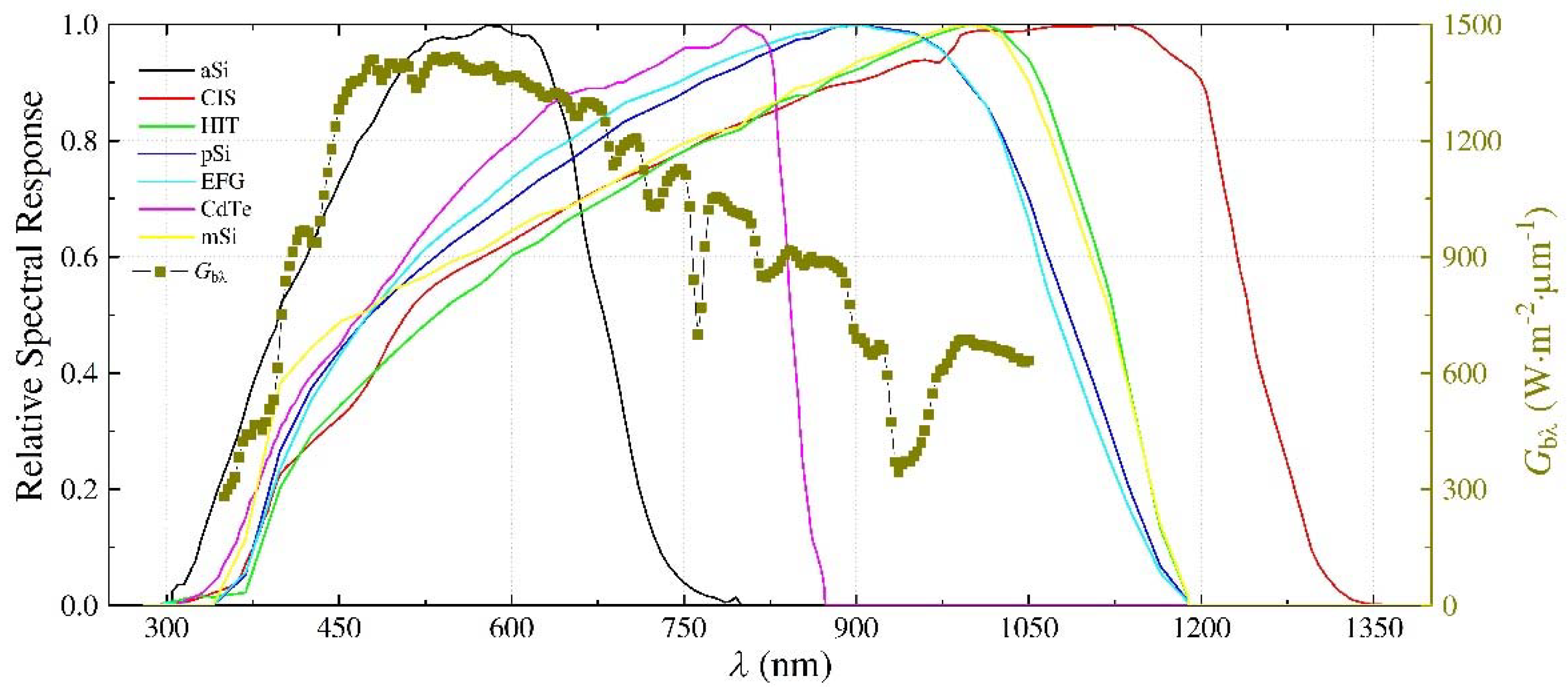Figure 1 shows the relative spectral response of seven PV technologies (as described in [5]) with wavelengths ranging from 300 nm to 1350 nm along with a common solar direct irradiance spectrum (G_bλ) measured in this work with a commercial spectroradiometer. The latter’s wavelength range is limited to 350−1050 nm and is thus not appropriate to evaluate the precise SF of most PV cells. Hence, the effect of the solar spectral distribution on the PV energy production cannot be accurately analysed with this typical instrumentation. The commercial combinations of two or more spectroradiometers do exist to achieve a much larger spectral range, as used at a small number of laboratories (see, e.g., [15]); however, the additional instrumentation is very costly, which makes it unavailable for most institutions.

Based on the above considerations, it appears that the ideal experimental avenue would require either spectroradiometers covering a wider spectral range (with the inconvenience of increasing costs) or the development of algorithms that would expand the limited spectrum sensed by usual spectroradiometers and provide a reasonable irradiance estimate over the entire shortwave spectrum. Here, the latter hybrid (measurement + model) approach is explored, using a new methodology based on the Simple Model of the Atmospheric Radiative Transfer of Sunshine (SMARTS) spectral code (version 2.9.8) [18] to achieve four complementary goals: (i) extend the wavelength range of measured direct irradiance spectra from ≈1050 nm up to 4000 nm; (ii) substantially improve the spectral resolution of the spectroradiometers (typically 7−10 nm) to 1 nm for the end product; (iii) provide accurate estimates of the clear-sky broadband irradiances incident on horizontal or tilted planes; (iv) evaluate the magnitude and variability of the abundance of various atmospheric constituents. The latter goal would normally require local (and expensive) remote-sensing instrumentation, which is rarely available at solar laboratories. Since the abundance of key atmospheric constituents, such as aerosols, water vapor, or ozone, must first be retrieved satisfactorily, this constitutes an interesting by-product in itself. In a second step, the expanded spectrum is calculated with SMARTS, using those retrievals.

The SMARTS model’s conceptual idea is to offer fast and accurate predictions of spectral irradiance on any tilted surface without the difficulties and limitations associated with the atmospheric models such as MODTRAN [19] or libRadtran [20], which require a large amount of atmospheric information that is often unavailable at the site of interest. The SMARTS model is now widely used worldwide in a large variety of applications. This is made possible by the model’s versatility and accuracy, which has been abundantly validated [21,22,23]. The model currently accommodates the case of cloudless skies only, for which it evaluates the clear-sky spectral irradiances (direct beam, circumsolar diffuse, hemispherical diffuse, and total on a prescribed receiver plane—tilted or horizontal) for specific atmospheric conditions (user specified or selected from 10 standard atmospheres), and for one-to-many points in time or solar geometries. The algorithms were developed to match the output from the sophisticated MODTRAN band models within ≈ 2 %. The algorithms are implemented in compiled FORTRAN code for various platforms and are used in conjunction with data files describing the spectral variation of surface albedo and of the absorption of atmospheric components. The spectral resolution is 0.5 nm from 280 nm to 400 nm, 1 nm from 400 nm to 1750 nm, and 10 nm from 1750 nm to 4000 nm. The version 2.9.8 used here is intended for education and research and is free for use for these intended applications.

2. Experimental Setup

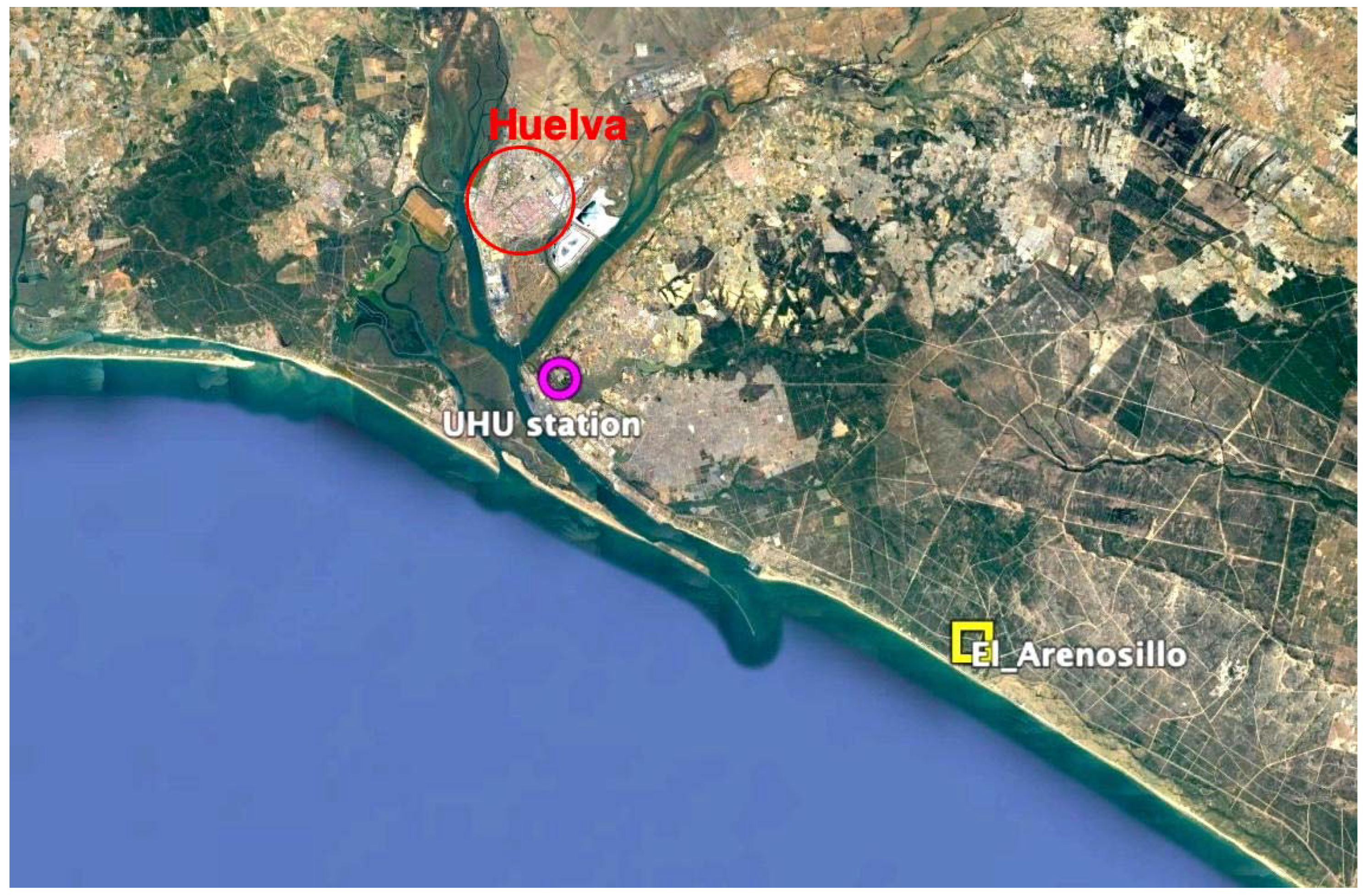
The experimental setup is located on a flat building roof of the High Technical School of Engineering on the Campus of La Rábida of the Universidad de Huelva (UHU), near Huelva (southwestern Spain), a seashore site within 5 km of the Atlantic Ocean (Figure 2). The aerosol species that are most frequent over the station region are coastal maritime, rural/continental, pollen, and desert dust [24].

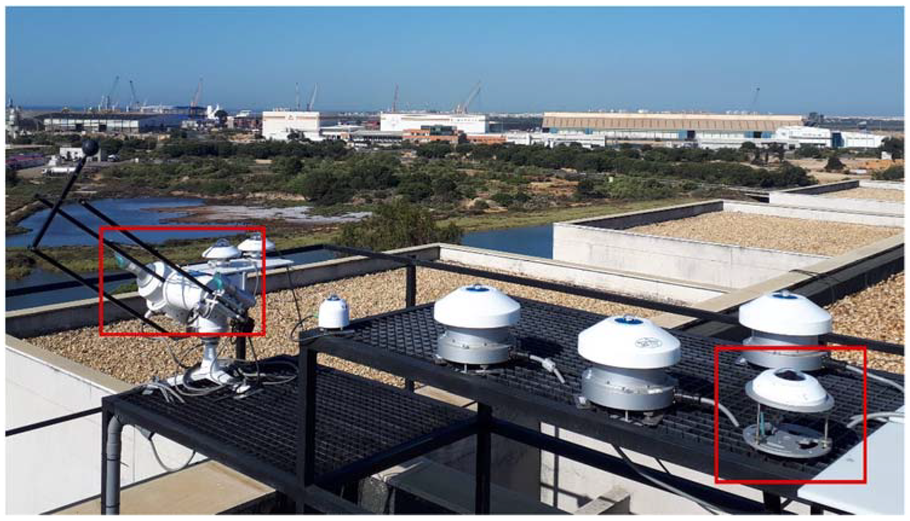
The experimental dataset consists of values of spectral beam normal irradiance (G_bλ), broadband global horizontal (G), broadband diffuse horizontal (G_d), and broadband direct normal (G_b) irradiances, as well as all-sky images and meteorological data (temperature, relative humidity, pressure, and wind speed), all of which have been collected since December 2020. G_bλ is measured at 5-min resolution using an MS-700N (EKO Instruments Co. Ltd., Tokyo, Japan) spectroradiometer equipped with a collimation tube. The instrument’s detector is a CCD array that covers the spectral range from 350 nm to 1050 nm with a wavelength interval of ≈3.3 nm, a spectral resolution of 10 nm, and a wavelength accuracy better than 0.3 nm. An EKO MS-56 pyrheliometer and two EKO MS-802 pyranometers (one of them blocking the sun by means of a shadow ball), separately sense the three essential components of solar radiation (G_b, G, and G_d, respectively). The spectral ranges that are sensed by the pyrheliometer and the pyranometers are (200−4000 nm) and (285−3000 nm, before absolute calibration), respectively. All these radiometers are mounted on an EKO STR-22G sun tracker.

The meteorological variables are measured with a WD-500 sensor manufactured by Lufft GmbH (Fellbach, Germany), and the sky images are taken using an EKO CMS ASI-16 All-Sky Imager. The latter is an automatic all-weather camera system with 180° field of view, using a 5-MP camera and a fish-eye lens with an anti-reflective, airflow protected, quartz dome. It delivers high-resolution images of the sky and clouds with a resolution of 1920 × 1920 pixels and 8-bit resolution per pixel. The horizon as seen by the ASI-16 is completely unshaded because the surroundings are at lower elevation.

Figure 3 shows the experimental setup, as installed on the flat roof of the building. The radiometric variables are sampled each second and are reported as 1-min averages. In parallel, the all-sky images and meteorological parameters are sampled every minute. All sensors are cleaned three days a week in the morning. Intercomparisons with unused radiometric sensors and several tests are carried out to guarantee the continuous quality of the broadband solar radiation measurements. The spectroradiometer is assumed to keep the original uncertainty provided by the manufacturer (<±18% for short wavelengths, improving to <±5% over the central part of the spectral range), or at least with an insignificant degradation of calibration, because the experimental period is short (less than two years, which is the calibration interval recommended by EKO).

Since one of the intermediate results derived from this work is the determination of some key aerosol optical properties (i.e., the aerosol optical depth at 500 nm, AOD₅₀₀, and the Ångström exponent, α) as well as the amount of water vapor (expressed as precipitable water, PW), the reference determinations of these variables were also obtained from a CE318 sunphotometer from Cimel (Paris, France), belonging to the AERONET network [25]. This instrument is located at the El Arenosillo Atmospheric Sounding Station (Instituto de Técnica Aeroespacial, INTA) in Mazagón (Huelva), another seashore site only ≈20 km away from the Campus of La Rábida. Figure 2 shows the location of the two stations.

Although many days of valid data are available, the present study focuses on only two cloudless days with very contrasting turbidity situations: one with a very clear sky (2021-03-24), characterized by minor aerosol load and low aerosol optical depth (AOD), and the other corresponding to hazy (highly turbid) conditions (2021-04-04). These sky conditions were selected manually by means of visual inspection of the daily evolution of solar radiation components and sky images (Figures 8 and 9). This process is time-consuming, which is why a long period of time (i.e., several months) is not included here. Nevertheless, an automatic procedure to discriminate between haze and cloudiness is currently being developed using the all-sky camera images [26]. This procedure is intended to become a reference for the selection of true cloudless sky conditions, in comparison with purely radiometric methods, which typically introduce some uncertainty [27]. In any case, a total of 20 spectra is used in this work to exemplify the procedure. Each experimental spectrum is sensed at 212 wavelengths, resulting in a total of 4240 spectral points. Nearly all of them are actively used in the retrieval procedure to extract the atmospheric properties of the moment. Hence, this amount is considered enough to ensure the reliability of the proposed methodology.

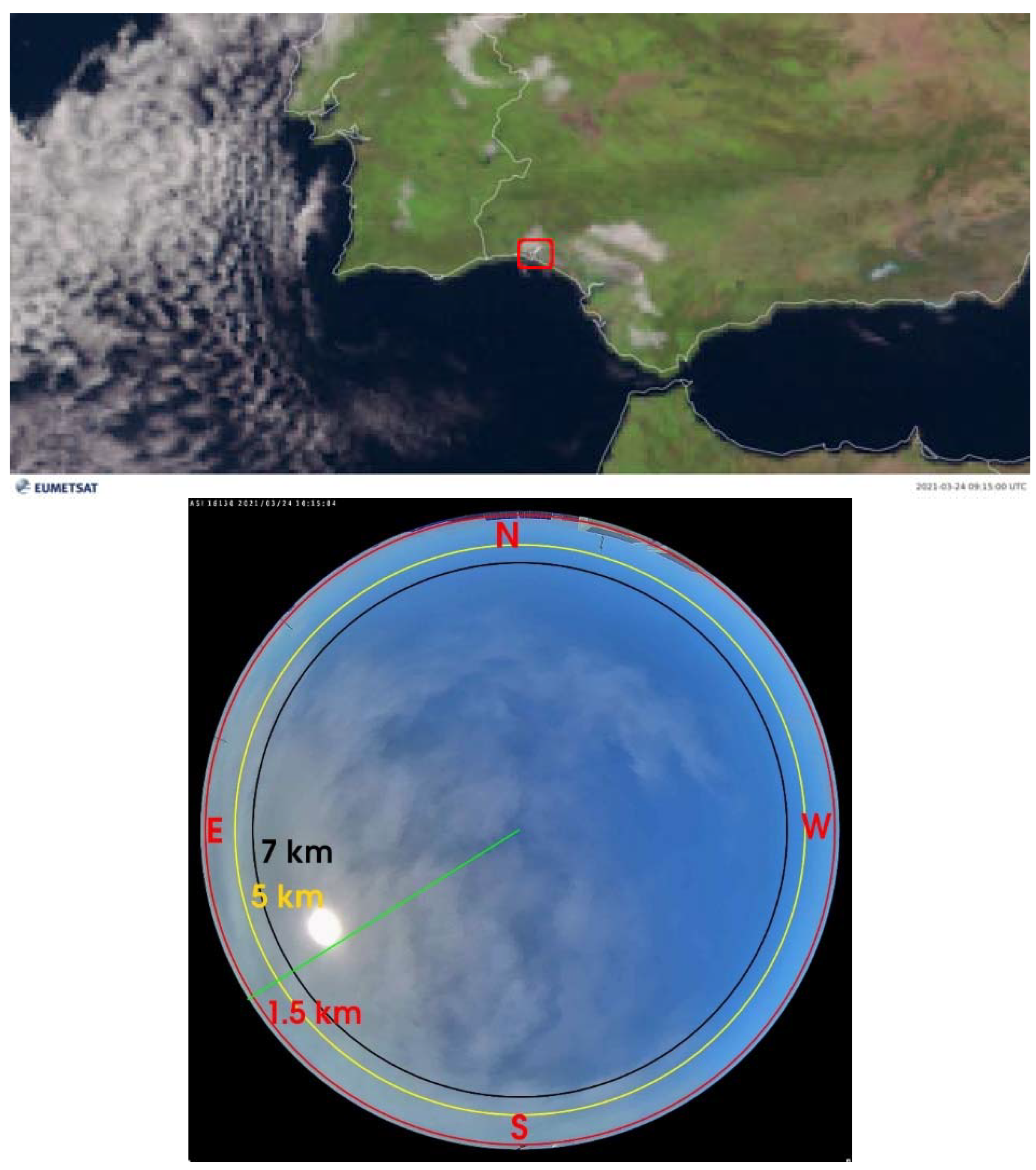
Remarkably, the atmospheric conditions that existed during the experiments at the UHU station also prevailed over the whole area of interest, including where the INTA-AERONET sunphotometer is located, as confirmed by the inspection of spaceborne imagery (such as those obtained using the EUMETSAT platform [28]) and aerosol data from MODIS. In this respect, Figure 4 (top) shows the area of interest (delimited by a red rectangle) as viewed by the Meteosat SEVIRI radiometer using an RGB natural-colour-enhanced product for one of the days selected in this work (2021-03-24) at 0915 UT. The presence of clouds is noted inside the red rectangle. The ASI-16 All-Sky Imager is also able to sense the sky over the El Arenosillo station. Figure 4 (bottom) shows a sky image corresponding to the same day and instant. Three circles are added, denoting three heights above ground (1.5 km, 5 km, and 7 km) and at a horizontal distance of 20 km from the imager. A green line marks the view direction to the El Arenosillo station. Low-level clouds over El Arenosillo would stand on the red circle at a mean height of ≈1.5 km above ground; mid-level clouds located at a mean height of ≈5 km would be seen on the yellow circle, and high-level clouds at ≈7 km would appear on the black circle. Nevertheless, the distance of clouds cannot be precisely determined from such sky images, since clouds at different horizontal distances from the All-Sky Imager with the same elevation angles are projected into the same pixel. However, if no clouds are present in the sky image, the same cloudless conditions would exist at both locations.

3. Methodology

The novel methodology proposed here attempts to obtain the specific values of the inputs to SMARTS that can, in turn, generate the modelled direct spectra that best fit their experimental counterpart. To this end, the variables to be estimated are either determined analytically or through a multistep iterative process, where they are varied incrementally between specific minimum and maximum limits until an optimum combination is found. Ultimately, for each instant when a measured spectrum is available, the modelled spectrum that is eventually selected is the one that results in the lowest root-mean-square error in comparison with its measured counterpart.

Each experimental direct spectrum is analysed to provide information about the atmospheric constituents in a way that is similar to what retrieval algorithms do for sunphotometric observations at, e.g., AERONET stations. In comparison, however, common CCD-array spectroradiometers, as with the one used here, normally have a coarser resolution (with irradiance at nearby wavelengths affecting each other) and are not calibrated against the sun; thus, they have a larger absolute uncertainty. These adverse conditions are compensated for here by using the guidance of a radiative transfer model and developing an appropriate iterative method. To be valid, the experimental spectra must be obtained under sky conditions characterized by a clear line of sight to the sun. This specific situation is comparable to what is obtained in similar remote-sensing (AERONET) retrievals after cloud screening, i.e., at level 1.5. This sky condition is much less stringent than a fully cloudless sky. Nevertheless, the latter prerequisite is actually implemented in this work for validation purposes because one way of verifying the method (see Section 4) consists of comparing the calculated and measured broadband diffuse and global irradiances, which are both very sensitive to cloudiness anywhere in the sky. For that specific purpose, the clear-sky condition is verified by visual inspection of the temporal variation of each broadband solar radiation component as well as by all-sky images. In the absence of an all-sky imager, both the cloudless and clear line-of-sight conditions can be identified a posteriori from broadband irradiance records using an advanced clear-sky detection algorithm [27].

The key inputs being incrementally varied in SMARTS, as well as their current acceptable limits, are given in

Table 1. Input values being varied in SMARTS and their range of tolerance for the fitting process.

Precipitable Water Content, PW (cm)	Ozone Content, uo (cm)	Air Quality (Trace Gases)	Ångström Exponent (α1, α2)	Turbidity (AOD500)
0.5–6.0	0.300–0.360	Pristine to Severe pollution	0.1–3.0	0.04–0.40

. Gueymard’s synthetic extraterrestrial spectrum (G_0λ) [29] is selected, corresponding to a solar constant of 1361.1 W/m². Default values are used for those inputs that do not affect the shortwave direct irradiance: CO₂ abundance (set here to 400 ppmv), aerosol’s single scattering albedo and asymmetry parameter (set to 0.9 and 0.7, respectively), and surface albedo (set to Light Soil). The pressure, temperature, and relative humidity inputs are normally measured; however, any missing value is estimated from the latitude and elevation of the site (37.20°N and 20 m a.m.s.l., respectively), along with the reference atmosphere, selected to be Mid-Latitude Summer (MLS) in the present case. The main radiatively active atmospheric quantities (AOD, α, PW, ozone, and air quality) are then derived iteratively to eventually determine the best combination of inputs, as described below.

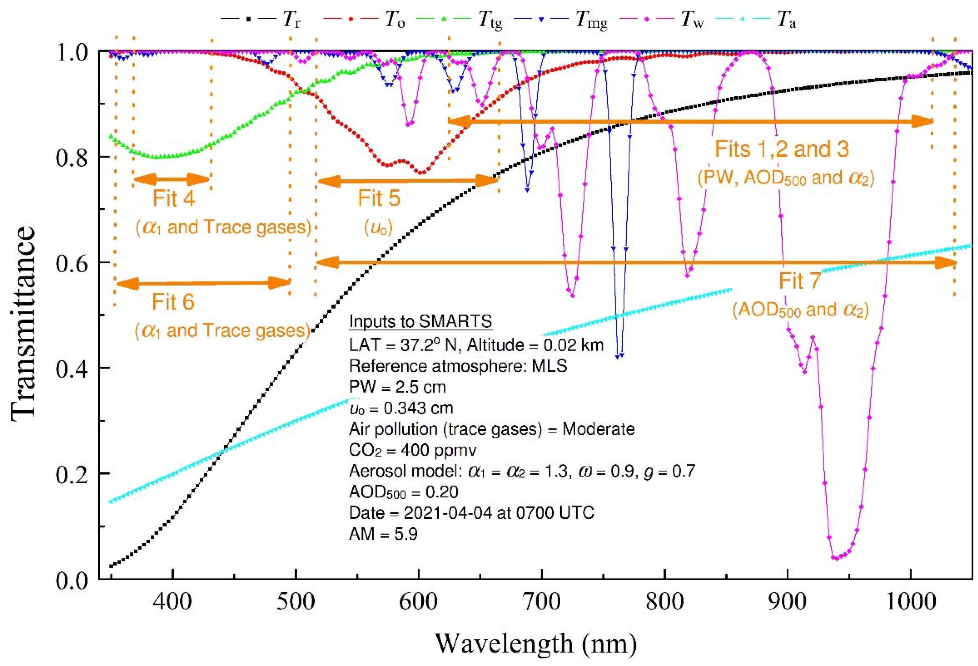
Figure 5 shows the transmittances corresponding to the atmospheric extinction processes used in SMARTS on 2021-04-04 at 0700 UTC. That specific low-sun moment (soon after sunrise) is characterized by an air mass (AM) higher than 5. This critical situation is intentionally selected here to observe the atmospheric effects on solar radiation when all extinction processes are enhanced by the longer atmospheric path. The transmittances provided by SMARTS are separately calculated for molecular (Rayleigh) scattering, T_r, ozone absorption, T_o, trace gases absorption, T_tg, mixed-gas absorption, T_mg, water vapor absorption, T_w, and aerosol scattering, T_a. The SMARTS spectral grid (2002 wavelengths between 280 nm and 4000 nm) has much finer intervals than the MS-700N grid (212 wavelengths between 350 nm and 1050 nm); moreover, the latter’s spectral resolution (≈10 nm full width at half maximum, FWHM) is much coarser than that of SMARTS. Hence, the smoothing of all SMARTS spectral outputs (through the application of an appropriate gaussian filter) is always necessary when any comparison with an experimental spectrum is made. Following this procedure, the SMARTS transmittances and spectra are progressively modified to closely match the experimental spectra provided by the spectroradiometer. A total of 212 observed spectral data points per spectrum is finally obtained between 350 nm and 1050 nm.

Figure 5 also shows several spectral bands (denoted by orange arrows) that are used as windows to calculate the best estimates for the SMARTS inputs, using an iterative fitting process consisting of 6 steps and 7 iterations, as detailed in the following subsections.

3.1. Step 1

The first step is conducted before the iterative fitting process and is intended to provide an initial and approximate value for both AOD₅₀₀ and the specific Ångström’s exponent for λ > 500 nm: α₂. The main reason for this preliminary analytic calculation is to save computer time, since an alternate iterative procedure could be excessively long (i.e., more than 10 min per spectrum) because convergence can be slow in that part of the spectrum.

Based on the data used in Figure 5, Figure 6 shows the total absorption transmittance obtained by removing the molecular and aerosol scattering, i.e., T_abs = T_Total/T_r·T_a = T_o·T_tg·T_mg·T_w. This is calculated over a very short spectral range (864.5−874.4 nm), which actually consists of only four wavelengths in the case of the MS-700N instrument: λ₁ = 864.5 nm, λ₂ = 867.8 nm, λ₃ = 871.1 nm, and λ₄ = 874.4 nm. Over that waveband (marked with a red rectangle in Figure 6), the total absorption transmittance is remarkably larger than 0.992 because the atmospheric attenuation of direct irradiance is mainly caused by molecular and aerosol scattering. Hence, for those wavelengths:

G_bλ ≈ G_0λ·T_r·T_a = G_0λ·T_r·exp(−m_a·AOD_λ),

(1)

where G_0λ is the extraterrestrial irradiance corrected for the actual sun–earth distance, m_a is the aerosol optical mass, and AOD_λ is the aerosol optical depth at wavelength λ. If measured values of G_bλ are used, all terms in the above equation are known, except for AOD_λ, since both T_r and m_a are only functions of solar position and pressure. Hence, AOD_λ can be calculated by solving Equation (1). Furthermore, based on Ångström’s equation, AOD₅₀₀ and α₂ can be evaluated if AOD_λ is known at any two wavelengths λ_a and λ_b:

$${\alpha }_2=\frac{{\lambda }_a}{{\lambda }_b}\mathrm{Ln}\left(\frac{{\mathrm{AOD}}_{\lambda a}}{{\mathrm{AOD}}_{\lambda b}}\right)$$

(2)

$${\mathrm{AOD}}_{500}={\mathrm{AOD}}_{\lambda }{\left(\frac{\lambda }{500}\right)}^{\alpha 2}$$

(3)

where wavelengths are expressed in nm. In Equation (2), better accuracy is obtained when λ_a and λ_b are spread as far as possible; hence, λ_a = 864.5 nm and λ_b = 874.4 nm. The near-centre wavelength of 867.8 nm is selected for λ. In what follows, these initial values are referred to as AOD₅₀₀(0) and α₂(0), respectively. They are ultimately refined at Step 6.

3.2. Step 2

The next step is to obtain a preliminary value for PW, and another set of estimates for AOD₅₀₀ and α₂. The spectral band selected here is 631.4−1011.6 nm, which contains 115 wavelengths in the case of the MS-700N instrument. In that range, the effect of trace gases is negligible (Figure 5). In addition, the ozone transmittance is not sensitive to small variations in total-column ozone abundance, u_o, which is initially set to the value of 0.34 cm that is used to define the reference AM1.5 spectra of STC [30]. Furthermore, the mixed-gas transmittance is well approximated with the selected reference atmosphere of Mid-Latitude Summer (MLS), along with the related inputs of latitude, elevation, date, and time. Two other SMARTS inputs, namely the Ångström exponent α₁ (defined for λ < 500 nm) and the abundance of trace gases, do not affect the current calculations and are thus defaulted to 1.3 and “light pollution”, respectively. To save computer time, the evaluation of PW, AOD₅₀₀, and α₂ is carried out by means of three consecutive fits (Fits #1, #2 and #3, as described in

Table 2. Initial values, maximum values, and increments for the estimation of three key SMARTS inputs when using iterative fits. The three consecutive fits are denoted as #1, #2, and #3.

Fit	PW (cm)			AOD500			α2
	Initial Value	Max.	Increment	Initial Value	Max.	Increment	Initial Value	Max.	Increment
#1	PW(0) = 0.5	6.0	0.5	AOD500(0)	—	—	α2(0) − 0.5	α2(0) + 0.5	0.1
#2	PW(#1) − 0.25	PW(#1) + 0.25	0.05	AOD500(0) − 0.06	AOD500(0) + 0.06	0.030	α2(#1) − 0.25	α2(0) + 0.25	0.02
#3	PW(#2) − 0.05	PW(#2) + 0.25	0.01	AOD500(0) − 0.015	AOD500(0) + 0.015	0.005	α2(#2) − 0.05	α2(0) + 0.05	0.015

and shown in Figure 5), where the corresponding intervals and maximum limits of the variables are progressively decreased. These estimates are labelled PW(#3), AOD₅₀₀(#3), and α₂(#3).

3.3. Step 3

The next unknowns to be estimated are α₁ and the trace-gases abundance. Figure 5 shows that there is a specific spectral band below 500 nm (namely, 369.9−426.8 nm), where the only attenuation is caused by aerosols and trace gases, because that of water vapor, ozone, and mixed gases is negligible. In this case, the fourth iterative fit (Fit #4 in Figure 5) is performed by varying α₁ from 0.2 to 3.0 in increments of 0.02 for each one of the four air-pollution (AP) models implemented into SMARTS. (The Huelva area is heavily industrialized and includes a chemical park with refineries, which is the biggest one in Spain; as such, local air pollution episodes are to be expected). The values obtained after the previous fit (#3) are used as inputs to Fit #4. Additionally, the ozone content is still defaulted to u_o = 0.34 cm.

3.4. Step 4

This step’s goal is to refine the ozone content through a fifth iterative fit (#5), where a short spectral band is selected (513.9 nm to 674.9 nm) and u_o is progressively increased from 0.28 cm to 0.365 cm in increments of 0.005 cm, while the others quantities are set to their previously found values: PW(#3), AOD₅₀₀(#3), α₁(#4), α₂(#3), and AP(#4).

3.5. Step 5

Once the ozone content is evaluated, the calculation of α₁ and the AP model is improved in a sixth iterative process (Fit #6), for which the selected spectral band (353.2−497.1 nm) is wider than that of Fit #4, while the number of wavelengths is increased from 18 to 44, and the spectral step is somewhat reduced. Now, α₁ is varied from α₁(#4) − 0.6 to α₁(#4) + 0.6 in increments of 0.01 for each of the four AP models.

3.6. Step 6

Finally, a last iteration (Fit #7) is performed in an attempt to improve the accuracy of the two critical aerosol parameters (AOD₅₀₀ and α₂), knowing the more realistic estimates for ozone, water vapor, and AP model obtained in previous steps. The spectral band is now 513.9−1037.4 nm and involves 158 wavelengths in the case of the MS-700N instrument. AOD₅₀₀ is varied from AOD₅₀₀(#3) − 0.01 to AOD₅₀₀(#3) + 0.01 in increments of 0.001, whereas α₂ is varied from α₂(#3) − 0.1 to α₂(#3) + 0.1 in increments of 0.01.

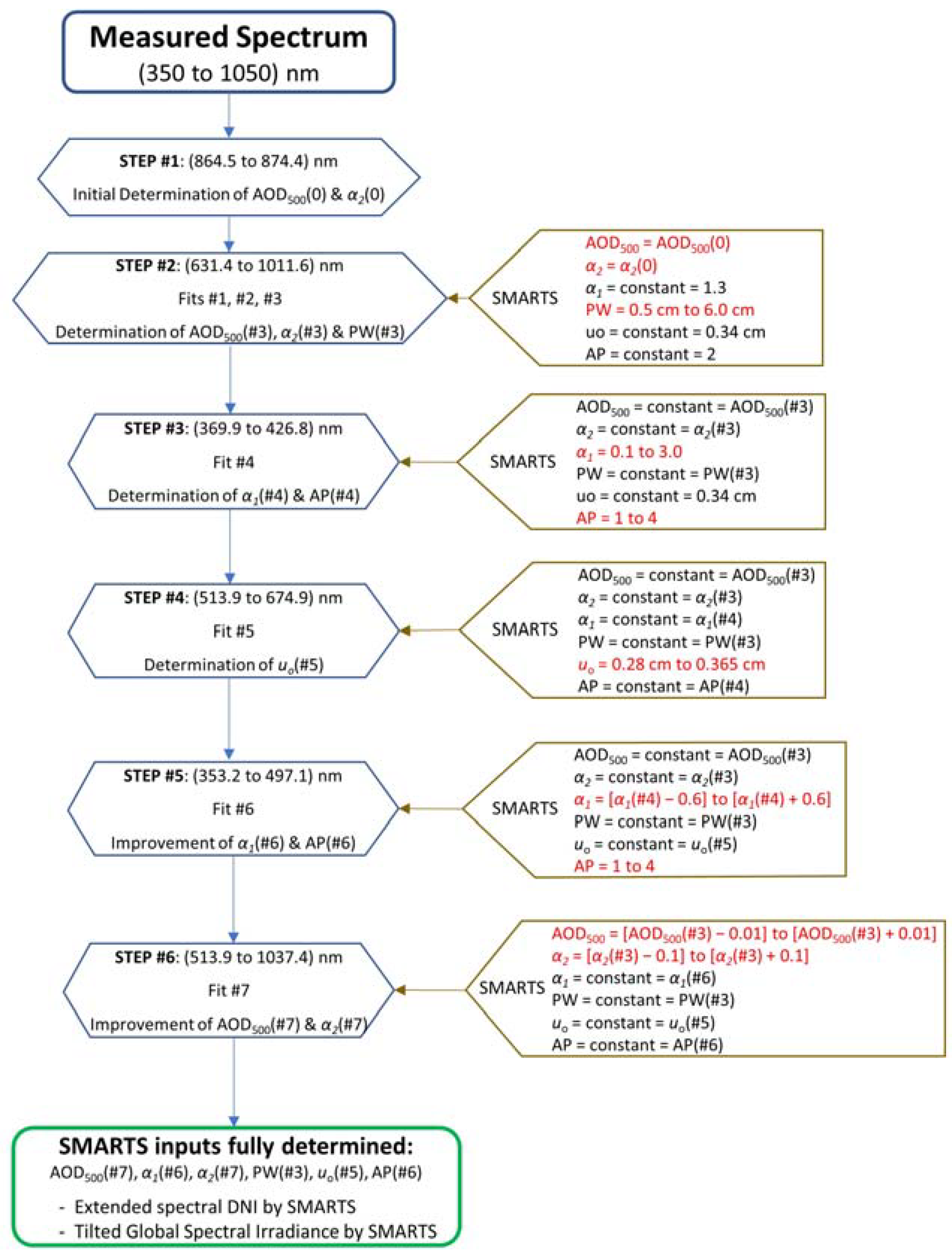
The overall input-fitting process and the successive steps are summarized in the flowchart shown in Figure 7. Remarkably, once the SMARTS inputs are properly evaluated for a given measured spectrum, it is then possible to obtain the extended (280−4000 nm) tilted global spectrum incident on a PV module, thus providing the necessary information to evaluate its output and performance.

4. Results

The procedure has been applied to a variety of situations during the whole experimental period. For the sake of brevity, only results pertaining to two contrasting atmospheric situations are detailed below. Each situation has been chosen randomly among a large pool of “very clear days” and “very hazy days”, i.e., very low and high AOD, respectively. This is key here because the direct spectrum is mostly impacted by AOD [18]. The results for all the other days that have been tested are similar to those presented here.

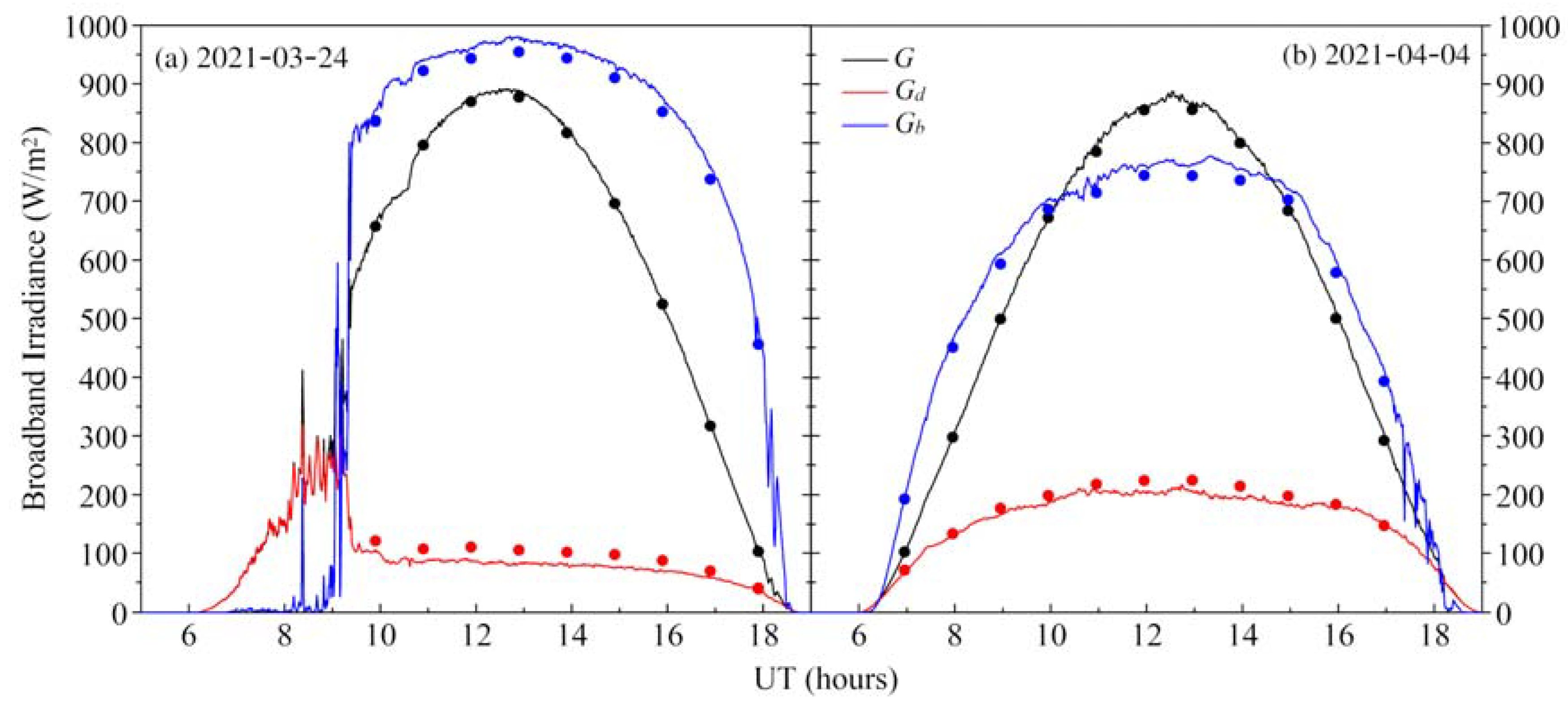
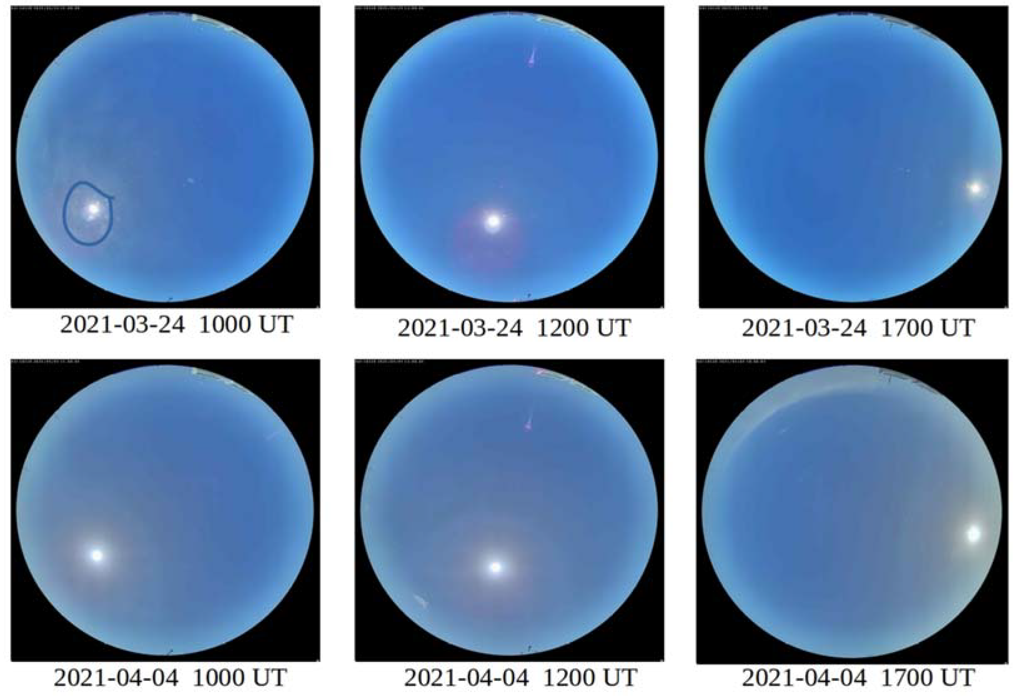
The diurnal evolution of the 1-min measured global, diffuse, and direct broadband irradiances is shown in Figure 8 for two contrasting days. It is apparent that differing atmospheric conditions existed during the cloudless parts of the two days, mostly related to changes in AOD. More precisely, the second day was hazier (i.e., had a higher AOD) than the first one, which translates into lower direct and higher diffuse irradiances. The first day was cloudy until ≈0930 UT. The cloudless periods of the two days have been selected after visual verification using the 1-min, all-sky images, as illustrated in Figure 9 for three different instants of each day. It is noted that, because of the hazier conditions, the second day’s sky colour is whiter than that of the first day. Moreover, a thin cloud (delimited by a blue line in the top left picture) was in front of the sun at 1000 UT of the first day. This was expected to lead to higher and erroneous estimates of AOD. Nevertheless, this instance was analysed for further reference.

The SMARTS-derived spectrum’s accuracy is evaluated by following the three independent procedures described below: (1) directly comparing the measured and estimated spectra; (2) comparing the measured and estimated broadband irradiances; (3) comparing the values of the estimated atmospheric parameters to those provided by a ground-based sunphotometer installed at the nearby AERONET site of El Arenosillo.

4.1. Spectrum Comparisons

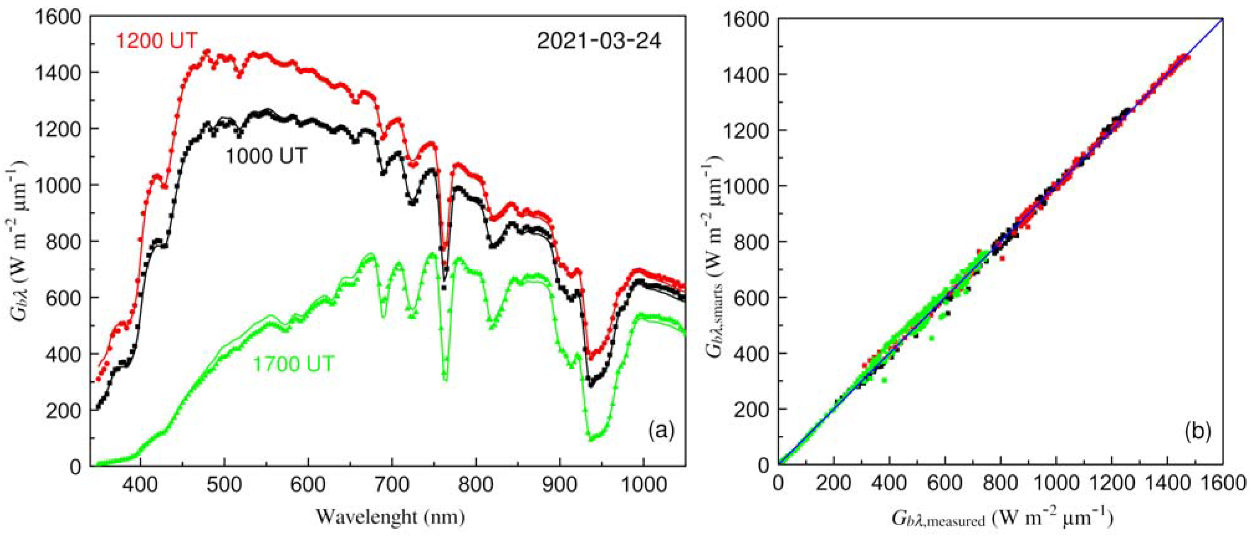
Figure 10a shows the measured direct spectrum along with the fitted spectral irradiance simulated by SMARTS for three different instants (0900, 1200, and 1700 UT) on 2021-03-24. The good agreement between the measured and modelled spectra is remarkable. To better evaluate the low deviations observed, Figure 10b provides a scatterplot of the spectral estimates versus the measured ones. Note the low scatter around the ideal straight line 1:1 of perfect fit. In fact, the root-mean-square errors (RMSEs) for almost all analysed instants are < 2 % for their 212 common wavelengths. The results found for the other day, 2021-04-04, are similar but are not shown for brevity.

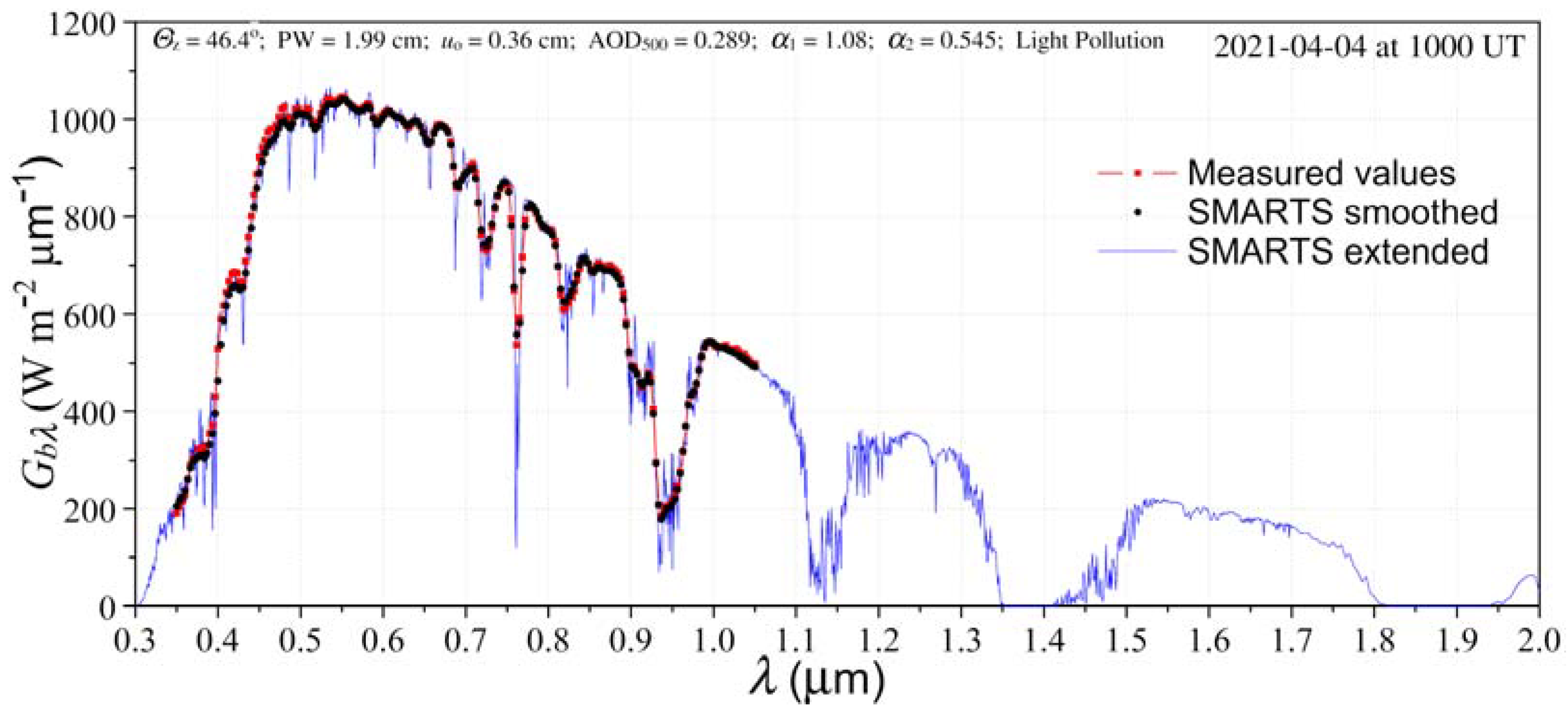
Figure 11 compares the spectral irradiance distributions from the spectroradiometer to the SMARTS-based estimates (after smoothing to match the instrument’s resolution) using the iterative procedure described above for day 2021-04-04 at 1000 UT. Again, the good agreement between these spectra is remarkable. In addition, Figure 11 also shows the SMARTS-derived spectrum at its native resolution of 0.5−5.0 nm between 280 nm and 4000 nm (2002 wavelengths). This extended version of the simulated spectrum significantly improves the resolution of the original experimental spectrum, which is a desirable feature in various applications and is necessary to accurately evaluate the corresponding broadband irradiance. Figure 7 shows such broadband values for the three irradiance components: total G, diffuse G_d, and direct G_b. Although a slight tendency to overestimate AOD seems to occur mainly in the middle part of the day (resulting in the direct and diffuse components being underestimated and overestimated, respectively), it is concluded that the agreement is more than satisfactory. This suggests that the proposed procedure is already reliable and efficient, at least for the range of atmospheric conditions investigated here.

4.2. AERONET Comparison

Although a complete analysis and comparison between the atmospheric characteristics derived in this work to those observed by a reference AERONET instrument is beyond the scope and extent of this work, a first and brief comparison between the two sets of values is discussed in this subsection for further reference.

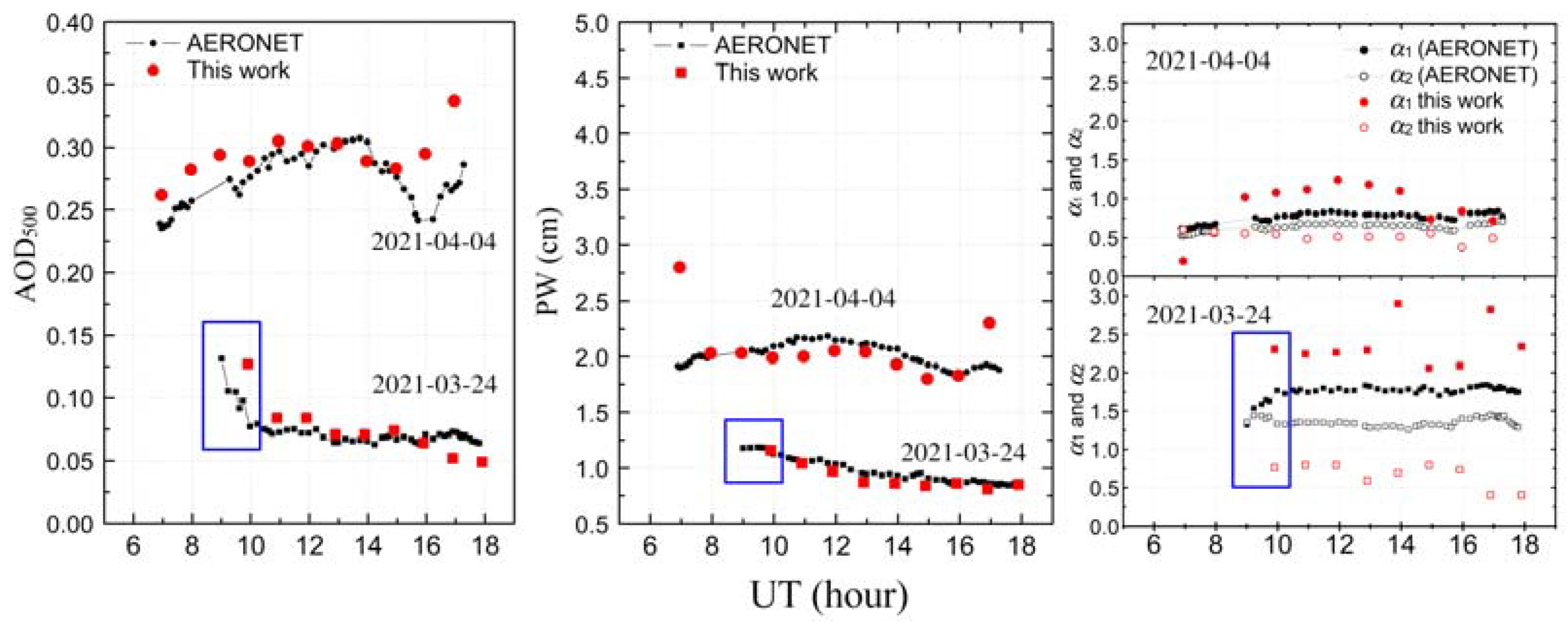
Figure 12 shows the diurnal variations of the retrieved values of PW, AOD₅₀₀, α₁, and α₂ throughout the two test days. The AOD₅₀₀ and PW estimates constitute a rather satisfactory match for the reference AERONET observations. This remarkable result is further confirmation of the adequacy of the retrieval method proposed here and suggests that a well-calibrated tracking spectroradiometer sensing the direct spectrum can be reasonably used as a substitute for a sunphotometer. Interestingly, the good agreement aforementioned for AOD₅₀₀ and PW is somewhat independent from the agreement found above for both spectral and broadband irradiances, because disparate sets of values can fortuitously be obtained if any one of the iteration processes leads to a local optimum rather than the true optimum. This adverse situation would prevent the iteration results from being similar to the AERONET retrievals, overwhelmingly considered in the literature as ‘ground-truth’ values. Hence, this AERONET-based validation constitutes a stringent way to evaluate the robustness and reliability of this new methodology.

As revealed in Figure 8 and Figure 9, some cloudiness interfered with the experiment during short periods of one test day. The method described above to retrieve the key atmospheric variables was conducted regardless, conditional to a non-zero direct irradiance. As expected, the retrieved AOD₅₀₀ was incorrectly too high since the sun’s disc is partially masked by a thin cloud, which adds its own optical depth. If such atmospheric retrievals were the main goal here, an a posteriori cloud-screening method would be necessary, such as the one routinely conducted on the AERONET raw data. Here, however, this issue is not a critical problem because the aim is to mimic the actual incident spectra on PV modules, even if affected by thin clouds.

In contrast with the good results mentioned above for AOD and PW, the Ångström exponents exhibit significant discrepancy, particularly during 2021-03-24. This appears to be related to the difficulty of obtaining a good representative value for these variables separately, possibly owing to the limited number of wavelengths for the two spectral bands. A single α value for the whole spectrum would simplify calculations and could be a better option; however, this has not been explored yet. From a different standpoint, it is also known that the determination of the Ångström parameter is difficult when AOD is low and generally prone to errors [31]. This can explain why their AERONET retrievals differ depending on the specific spectral band (and number of wavelengths) used for their derivation. Additional studies are definitely needed to improve this specific retrieval. Fortunately, though, any reasonable error here does not significantly impact the robustness of the extended spectra, as shown in Figure 11.

5. Conclusions

Low-cost spectroradiometers are currently being manufactured to monitor the spectral solar irradiance and are frequently used for PV research purposes at many solar laboratories. A usual drawback of these devices is their limited spectral range and/or relatively coarse optical resolution. These issues might hinder their usefulness in specific applications, such as the retrieval of atmospheric parameters or the study of PV spectral effects, where a wider spectral band is required because the spectral response of the PV cells under scrutiny extends beyond the range covered by the spectroradiometer.

The novel methodology proposed here offers an efficient and accurate way to extend the direct spectrum observed by spectroradiometers under clear-sky conditions. Both the spectral range and resolution of the original measured spectrum are improved using the simulations provided by the SMARTS spectral code. To that effect, an iterative procedure is developed to estimate the most important SMARTS atmospheric inputs through a succession of least-square fits. Once these SMARTS inputs are established, direct spectra ranging from 280 nm to 4000 nm and with a resolution of 0.5 nm to 5.0 nm (depending on waveband) can be simulated. This is particularly useful if spectra are needed for the other (diffuse and global) solar radiation components, or are needed for tilted surfaces, which is particularly important in the case of PV studies.

The results obtained here have also shown that, in addition to obtaining accurate spectral simulations, the new methodology is able to provide reliable estimates for the essential atmospheric quantities, such as precipitable water or aerosol optical depth at 500 nm. Ultimately, this suggests that tracking spectroradiometers sensing the direct spectrum could be used to monitor atmospheric constituents with an accuracy potentially comparable to that of sunphotometers under cloudless conditions.

Nevertheless, this procedure still needs refinements and to be further validated using data from a variety of locations, during longer periods, and with a wider range of atmospheric conditions. Optimization of the iteration algorithms will also be necessary to decrease the computation time, which is still substantial.