
Reusing Remote Sensing-Based Validation Data: Comparing Direct and Indirect Approaches for Afforestation Monitoring

 ,
,  ,
,  ,
,  , , and
Abstract
1. Introduction
2. Materials and Methods
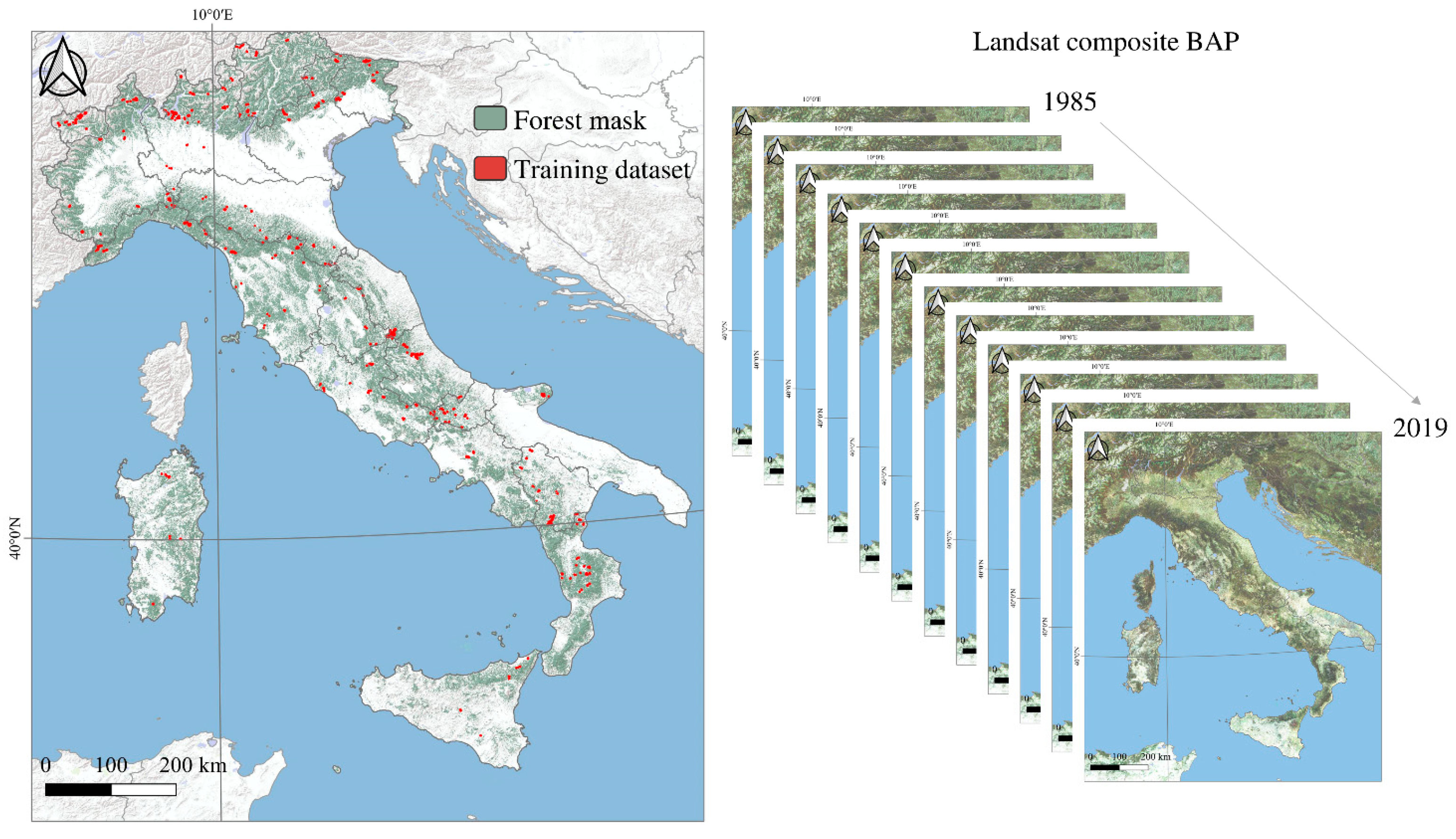
2.1. Study Area and Forest Mask
2.2. Landsat Best Available Composite Imagery
2.3. Training Dataset
- 526 polygons (A) that experienced a change from non-forest to forest in the period 1985–2020,
- 526 polygons (B) in non-forest areas that did not change between 1985 and 2020
- 526 polygons (C) in forest areas that did not change between 1985 and 2020.
3. Methods
3.1. Direct and Indirect Afforestation Map Construction
3.2. First and Second Phases of Validation Data Selection
3.3. Validation Data Adjustment Phase
3.4. Accuracy Assessment
4. Results
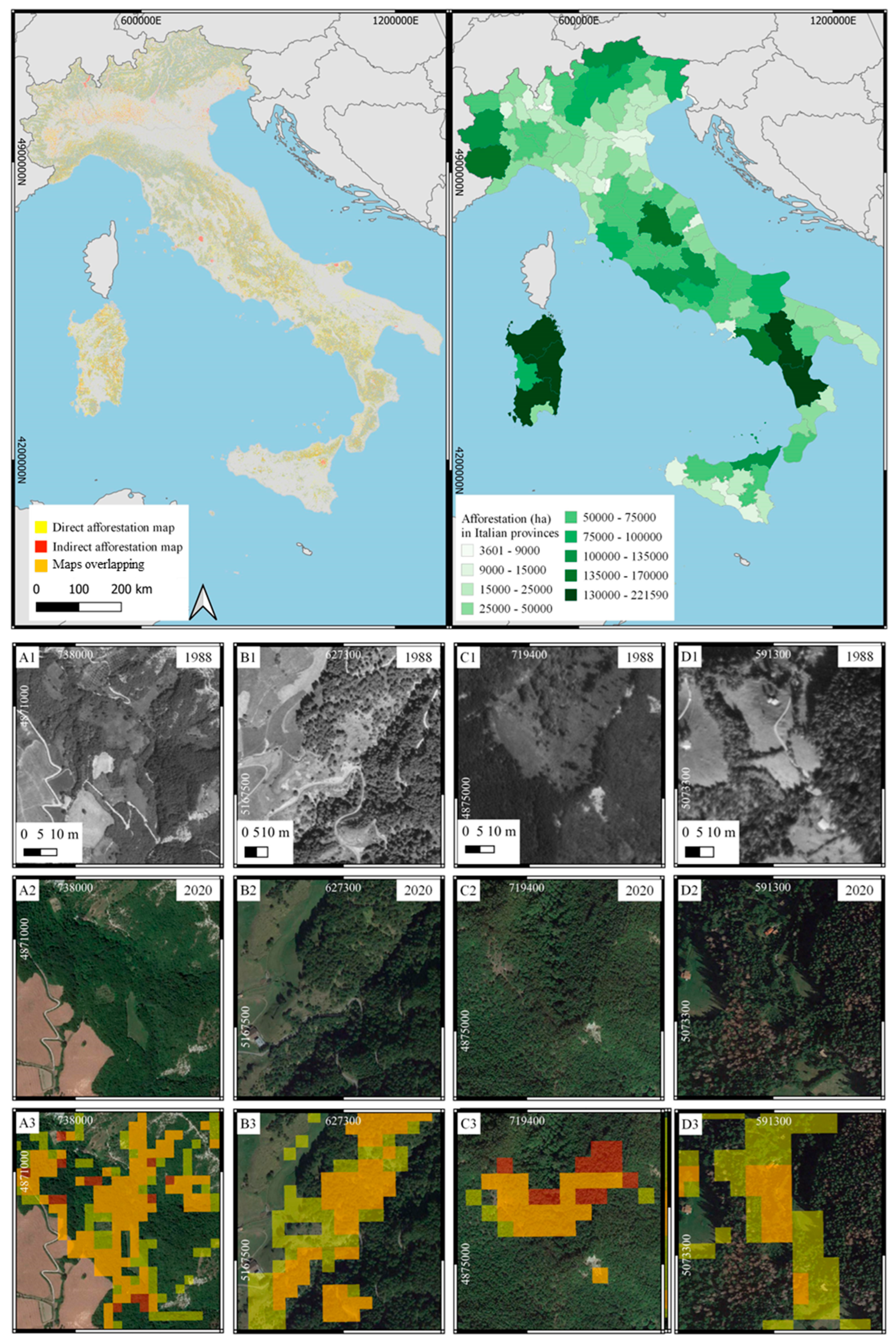
4.1. Direct and Indirect Afforestation Maps
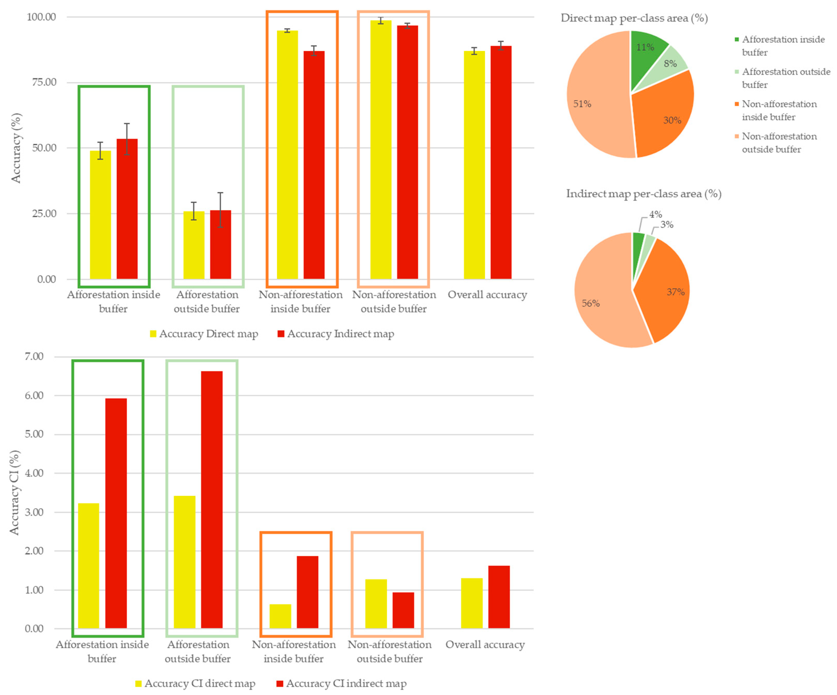
4.2. Direct and Indirect Map Accuracy Comparisons
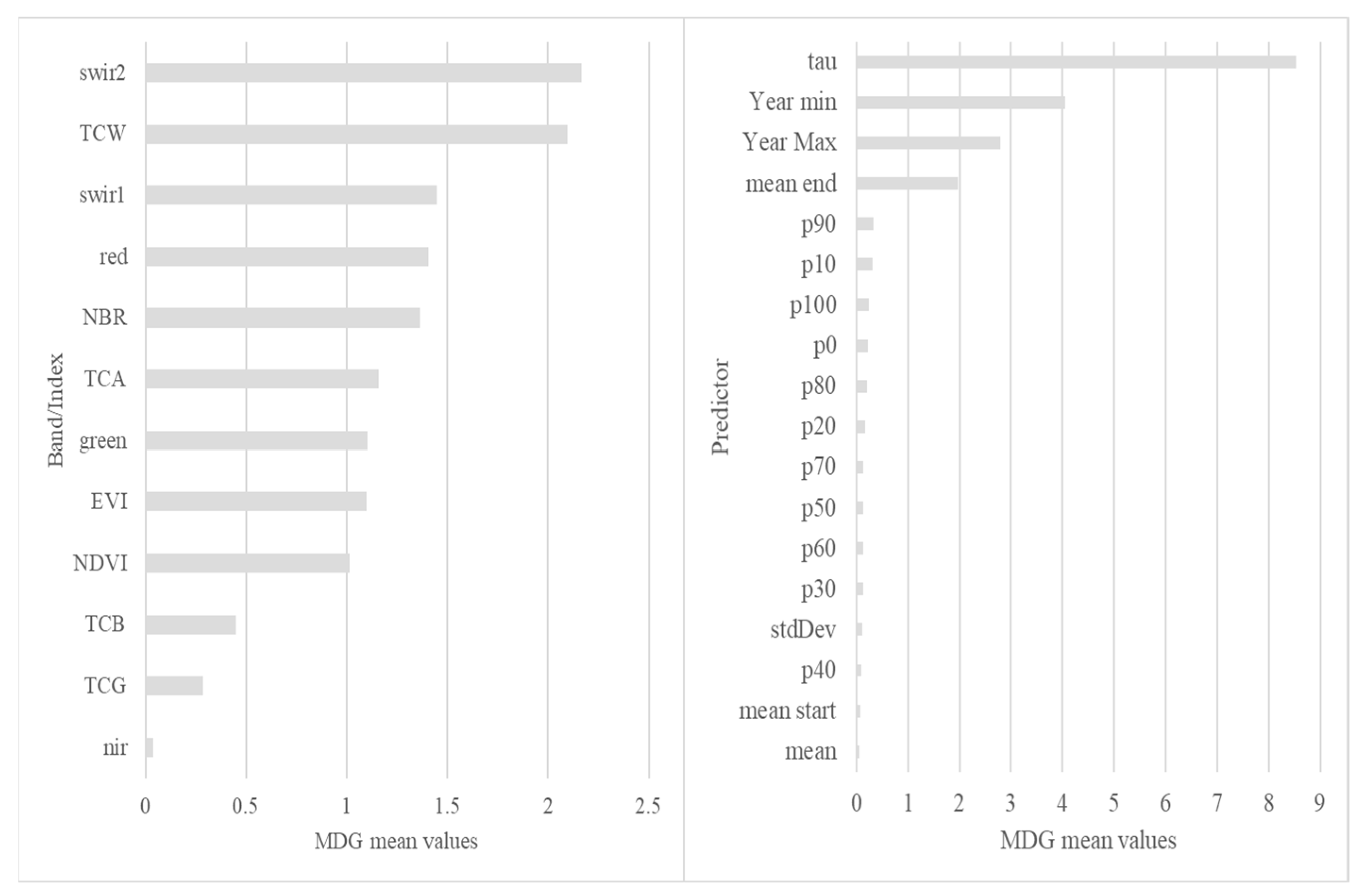
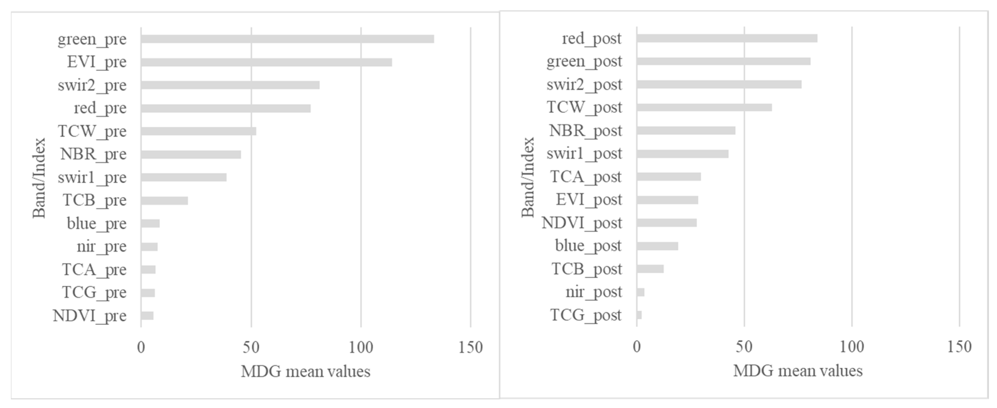
4.3. RF Variable Importance Ranking in Direct and Indirect Approach
5. Discussion
5.1. Contextualization of the Study
5.2. Summary of the Issues We Addressed and How We Did So
5.3. Validation Ample Adjustment Method
5.4. Map Accuracy
5.5. Variable Importance Ranking
6. Conclusions
Author Contributions
Funding
Acknowledgments
Conflicts of Interest
Appendix A

| Map Class | Validation Data | Sum | |||||
|---|---|---|---|---|---|---|---|
| Afforestation | Non- Afforestation | ||||||
| Afforestation inside buffer | 418 | 436 | 854 | 0.11 | 0.49 | 0.05 | 3.24 |
| Afforestation outside buffer | 191 | 544 | 735 | 0.08 | 0.26 | 0.02 | 3.42 |
| Non-afforestation inside buffer | 61 | 1130 | 1191 | 0.30 | 0.95 | 0.29 | 0.64 |
| Non-afforestation outside buffer | 16 | 1225 | 1241 | 0.52 | 0.99 | 0.51 | 1.28 |
| Overall Accuracy | 87% | 1.33 | |||||
| Maps Classes Combination | Validation Data | Sum | ||||||
|---|---|---|---|---|---|---|---|---|
| Indirect | Direct | Afforestation | Non- Afforestation | |||||
| Afforestation inside buffer | Afforestation inside buffer | 163 | 119 | 282 | 0.04 | 0.58 | 0.02 | 5.88 |
| Afforestation inside buffer | Non-afforestation inside buffer | 1 | 29 | 30 | 0.00 | 0.03 | 0.00 | 6.55 |
| Afforestation outside buffer | Afforestation outside buffer | 70 | 133 | 203 | 0.02 | 0.34 | 0.01 | 6.67 |
| Afforestation outside buffer | Non-afforestation outside buffer | 1 | 29 | 30 | 0.01 | 0.03 | 0.00 | 6.55 |
| Non-afforestation inside buffer | Afforestation inside buffer | 255 | 317 | 572 | 0.07 | 0.55 | 0.04 | 4.16 |
| Non-afforestation inside buffer | Non-afforestation inside buffer | 60 | 1101 | 1161 | 0.30 | 0.95 | 0.28 | 1.30 |
| Non-afforestation outside buffer | Afforestation outside buffer | 121 | 411 | 532 | 0.05 | 0.77 | 0.04 | 3.63 |
| Non-afforestation outside buffer | Non-afforestation outside buffer | 15 | 1196 | 1211 | 0.51 | 0.99 | 0.50 | 0.64 |
| Overall accuracy | 89% | 1.62 | ||||||
| Maps Classes Combination | Validation Data | Sum | Class Accuracy % | |||||||
|---|---|---|---|---|---|---|---|---|---|---|
| Indirect | Direct | Afforestation | Non- afforest ation | |||||||
| Afforestation inside buffer | Afforestation inside buffer | 163 | 119 | 282 | 13,909,582 | 0.92 | 0.58 | 0.53 | 5.88 | |
| Afforestation inside buffer | Non-afforestation inside buffer | 1 | 29 | 30 | 1,195,672 | 0.08 | 0.03 | 0.00 | 6.55 | |
| Afforestation inside buffer | 15,105,254 | #3 53 | 5.93 #4 | |||||||
| Afforestation outside buffer | Afforestation outside buffer | 70 | 133 | 203 | 9,245,508 | 0.75 | 0.34 | 0.26 | 6.65 | |
| Afforestation outside buffer | Non-afforestation outside buffer | 1 | 29 | 30 | 3,053,527 | 0.25 | 0.03 | 0.01 | 6.55 | |
| Afforestation outside buffer | 12,299,035 | #3 27 | 6.63 #4 | |||||||
| Non-afforestation inside buffer | Afforestation inside buffer | 255 | 317 | 572 | 28,589,586 | 0.20 | 0.55 | 0.11 | 4.16 | |
| Non-afforestation inside buffer | Non-afforestation inside buffer | 60 | 1101 | 1161 | 117,906,305 | 0.80 | 0.95 | 0.76 | 1.30 | |
| Non-afforestation inside buffer | 146,495,891 | #3 87 | 1.87 #4 | |||||||
| Non-afforestation outside buffer | Afforestation outside buffer | 121 | 411 | 532 | 21,365,513 | 0.10 | 0.77 | 0.07 | 3.63 | |
| Non-afforestation outside buffer | Non-afforestation outside buffer | 15 | 1196 | 1211 | 201,081,401 | 0.90 | 0.99 | 0.89 | 0.64 | |
| Non-afforestation outside buffer | 222,446,914 | #3 97 | 0.94 #4 | |||||||
References
- Intergovernamental Panel on Climate Change (IPCC). Climate Change 2021 The Physical Science Basis; IPCC: Nykoping, Sweden, 2021. [Google Scholar]
- FAO. Global Forest Resources Assessment 2020—Guidelines and Specifications. Forest Resources Assessment; FAO: Rome, Italy, 2020; Volume 42. [Google Scholar]
- Gorelick, N.; Hancher, M.; Dixon, M.; Ilyushchenko, S.; Thau, D.; Moore, R. Google Earth Engine: Planetary-scale geospatial analysis for everyone. Remote Sens. Environ. 2017, 202, 18–27. [Google Scholar] [CrossRef]
- Wulder, M.A.; Coops, N.C. Satellites: Make Earth observations open access. Nature 2014, 513, 30–31. [Google Scholar] [CrossRef]
- Francini, S.; Chirici, G. A Sentinel-2 derived dataset of forest disturbances occurred in Italy between 2017 and 2020. Data Brief 2022, 42, 108297. [Google Scholar] [CrossRef] [PubMed]
- Nabuurs, G.-J.; Harris, N.; Sheil, D.; Palahi, M.; Chirici, G.; Boissière, M.; Fay, C.; Reiche, J.; Valbuena, R. Glasgow forest declaration needs new modes of data ownership. Nat. Clim. Change 2022, 12, 415–417. [Google Scholar] [CrossRef]
- Gomes, V.C.F.; Queiroz, G.R.; Ferreira, K.R. An Overview of Platforms for Big Earth Observation Data Management and Analysis. Remote Sens. 2020, 12, 1253. [Google Scholar] [CrossRef]
- Wulder, M.A.; Loveland, T.R.; Roy, D.P.; Crawford, C.J.; Masek, J.G.; Woodcock, C.E.; Allen, R.G.; Anderson, M.C.; Belward, A.S.; Cohen, W.B.; et al. Current status of Landsat program, science, and applications. Remote Sens. Environ. 2019, 225, 127–147. [Google Scholar] [CrossRef]
- Wulder, M.A.; Masek, J.G.; Cohen, W.B.; Loveland, T.R.; Woodcock, C.E. Opening the archive: How free data has enabled the science and monitoring promise of Landsat. Remote Sens. Environ. 2012, 122, 2–10. [Google Scholar] [CrossRef]
- Breiman, L. Random forests. Mach. Learn. 2001, 45, 5–32. [Google Scholar] [CrossRef]
- Hawryło, P.; Francini, S.; Chirici, G.; Giannetti, F.; Parkitna, K.; Krok, G.; Mitelsztedt, K.; Lisańczuk, M.; Stereńczak, K.; Ciesielski, M.; et al. The Use of Remotely Sensed Data and Polish NFI Plots for Prediction of Growing Stock Volume Using Different Predictive Methods. Remote Sens. 2020, 12, 3331. [Google Scholar] [CrossRef]
- Belgiu, M.; Drăguţ, L. Random forest in remote sensing: A review of applications and future directions. ISPRS J. Photogramm. Remote Sens. 2016, 114, 24–31. [Google Scholar] [CrossRef]
- Vangi, E.; D’Amico, G.; Francini, S.; Giannetti, F.; Lasserre, B.; Marchetti, M.; McRoberts, R.E.; Chirici, G. The Effect of Forest Mask Quality in the Wall-to-Wall Estimation of Growing Stock Volume. Remote Sens. 2021, 13, 1038. [Google Scholar] [CrossRef]
- Hermosilla, T.; Bastyr, A.; Coops, N.C.; White, J.C.; Wulder, M.A. Mapping the presence and distribution of tree species in Canada’s forested ecosystems. Remote Sens. Environ. 2022, 282, 113276. [Google Scholar] [CrossRef]
- McRoberts, R.E.; Næsset, E.; Gobakken, T.; Bollandsås, O.M. Indirect and direct estimation of forest biomass change using forest inventory and airborne laser scanning data. Remote Sens. Environ. 2015, 164, 36–42. [Google Scholar] [CrossRef]
- Bollandsås, O.M.; Gregoire, T.G.; Næsset, E.; Øyen, B.-H. Detection of biomass change in a Norwegian mountain forest area using small footprint airborne laser scanner data. Stat. Methods Appl. 2013, 22, 113–129. [Google Scholar] [CrossRef]
- Fuller, R.M.; Smith, G.M.; Devereux, B.J. The characterisation and measurement of land cover change through remote sensing: Problems in operational applications? Int. J. Appl. Earth Obs. Geoinf. 2003, 4, 243–253. [Google Scholar] [CrossRef]
- Skowronski, N.S.; Clark, K.L.; Gallagher, M.; Birdsey, R.A.; Hom, J.L. Airborne laser scanner-assisted estimation of aboveground biomass change in a temperate oak–pine forest. Remote Sens. Environ. 2014, 151, 166–174. [Google Scholar] [CrossRef]
- Qiu, B.; Zou, F.; Chen, C.; Tang, Z.; Zhong, J.; Yan, X. Automatic mapping afforestation, cropland reclamation and variations in cropping intensity in central east China during 2001–2016. Ecol. Indic. 2018, 91, 490–502. [Google Scholar] [CrossRef]
- Ramírez-Cuesta, J.M.; Minacapilli, M.; Motisi, A.; Consoli, S.; Intrigliolo, D.S.; Vanella, D. Characterization of the main land processes occurring in Europe (2000–2018) through a MODIS NDVI seasonal parameter-based procedure. Sci. Total. Environ. 2021, 799, 149346. [Google Scholar] [CrossRef]
- Yin, H.; Pflugmacher, D.; Li, A.; Li, Z.; Hostert, P. Land use and land cover change in Inner Mongolia—Understanding the effects of China’s re-vegetation programs. Remote Sens. Environ. 2018, 204, 918–930. [Google Scholar] [CrossRef]
- Haller, A.; Bender, O. Among rewilding mountains: Grassland conservation and abandoned settlements in the Northern Apennines. Landsc. Res. 2018, 43, 1068–1084. [Google Scholar] [CrossRef]
- Cavalli, A.; Francini, S.; McRoberts, R.E.; Falanga, V.; Congedo, L.; de Fioravante, P.; Maesano, M.; Munafò, M.; Chirici, G.; Mugnozza, G.S. Estimating Afforestation Area Using Landsat Time Series and Photointerpreted Datasets. Remote Sens. 2022, 15, 923. [Google Scholar] [CrossRef]
- Shen, W.; Li, M.; Huang, C.; Tao, X.; Li, S.; Wei, A. Mapping Annual Forest Change Due to Afforestation in Guangdong Province of China Using Active and Passive Remote Sensing Data. Remote Sens. 2019, 11, 490. [Google Scholar] [CrossRef]
- Townshend, J.R.; Masek, J.G.; Huang, C.; Vermote, E.F.; Gao, F.; Channan, S.; Sexton, J.O.; Feng, M.; Narasimhan, R.; Kim, D.; et al. Global characterization and monitoring of forest cover using Landsat data: Opportunities and challenges. Int. J. Digit. Earth 2012, 5, 373–397. [Google Scholar] [CrossRef]
- McRoberts, R.E.; Bollandsås, O.M.; Næsset, E. Modeling and Estimating Change BT—Forestry Applications of Airborne Laser Scanning: Concepts and Case Studies; Maltamo, M., Næsset, E., Vauhkonen, J., Eds.; Springer Netherlands: Dordrecht, The Netherlands, 2014; pp. 293–313. ISBN 978-94-017-8663-8. [Google Scholar]
- Olofsson, P.; Foody, G.M.; Stehman, S.V.; Woodcock, C.E. Making better use of accuracy data in land change studies: Estimating accuracy and area and quantifying uncertainty using stratified estimation. Remote Sens. Environ. 2013, 129, 122–131. [Google Scholar] [CrossRef]
- Fattorini, L. Design-based methodological advances to support national forest inventories: A review of recent proposals. iForest—Biogeosci. For. 2014, 8, 6–11. [Google Scholar] [CrossRef]
- Stehman, S.V. Practical Implications of Design-Based Sampling Inference for Thematic Map Accuracy Assessment. Remote Sens. Environ. 2000, 72, 35–45. [Google Scholar] [CrossRef]
- Francini, S.; McRoberts, R.E.; D’Amico, G.; Coops, N.C.; Hermosilla, T.; White, J.C.; Wulder, M.A.; Marchetti, M.; Mugnozza, G.S.; Chirici, G. An open science and open data approach for the statistically robust estimation of forest disturbance areas. Int. J. Appl. Earth Obs. Geoinf. 2022, 106, 102663. [Google Scholar] [CrossRef]
- Francini, S.; D’Amico, G.; Mencucci, M.; Seri, G.; Gravano, E.; Chirici, G. Remote sensing and automatic procedures: Useful tools to monitor forest harvesting. For.—Riv. Selvic. Ecol. For. 2021, 18, 27–34. [Google Scholar] [CrossRef]
- Stehman, S.V.; Czaplewski, R.L. Design and Analysis for Thematic Map Accuracy Assessment—An Application of Satellite Imagery. Remote Sens. Environ. 1998, 64, 331–344. [Google Scholar] [CrossRef]
- D’Amico, G.; Vangi, E.; Francini, S.; Giannetti, F.; Nicolaci, A.; Travaglini, D.; Massai, L.; Giambastiani, Y.; Terranova, C.; Chirici, G. Are we ready for a National Forest Information System? State of the art of forest maps and airborne laser scanning data availability in Italy. iForest—Biogeosci. For. 2021, 14, 144–154. [Google Scholar] [CrossRef]
- White, J.C.; Wulder, M.A.; Hobart, G.W.; Luther, J.E.; Hermosilla, T.; Griffiths, P.; Coops, N.C.; Hall, R.J.; Hostert, P.; Dyk, A.; et al. Pixel-Based Image Compositing for Large-Area Dense Time Series Applications and Science. Can. J. Remote Sens. 2014, 40, 192–212. [Google Scholar] [CrossRef]
- Griffiths, P.; van der Linden, S.; Kuemmerle, T.; Hostert, P. Erratum: A Pixel-Based Landsat Compositing Algorithm for Large Area Land Cover Mapping. IEEE J. Sel. Top. Appl. Earth Obs. Remote Sens. 2013, 6, 2088–2101. [Google Scholar] [CrossRef]
- Francini, S.; D’Amico, G.; Vangi, E.; Borghi, C.; Chirici, G. Integrating GEDI and Landsat: Spaceborne Lidar and Four Decades of Optical Imagery for the Analysis of Forest Disturbances and Biomass Changes in Italy. Sensors 2022, 22, 2015. [Google Scholar] [CrossRef] [PubMed]
- White, J.C.; Wulder, M.A.; Hermosilla, T.; Coops, N.C.; Hobart, G.W. A nationwide annual characterization of 25 years of forest disturbance and recovery for Canada using Landsat time series. Remote Sens. Environ. 2017, 194, 303–321. [Google Scholar] [CrossRef]
- Hermosilla, T.; Wulder, M.A.; White, J.C.; Coops, N.C.; Hobart, G.W. An integrated Landsat time series protocol for change detection and generation of annual gap-free surface reflectance composites. Remote Sens. Environ. 2015, 158, 220–234. [Google Scholar] [CrossRef]
- Hermosilla, T.; Wulder, M.A.; White, J.C.; Coops, N.C.; Hobart, G.W. Regional detection, characterization, and attribution of annual forest change from 1984 to 2012 using Landsat-derived time-series metrics. Remote Sens. Environ. 2015, 170, 121–132. [Google Scholar] [CrossRef]
- Jönsson, P.; Cai, Z.; Melaas, E.; Friedl, M.A.; Eklundh, L. A Method for Robust Estimation of Vegetation Seasonality from Landsat and Sentinel-2 Time Series Data. Remote Sens. 2018, 10, 635. [Google Scholar] [CrossRef]
- Roy, D.P.; Boschetti, L.; Trigg, S.N. Remote Sensing of Fire Severity: Assessing the Performance of the Normalized Burn Ratio. IEEE Geosci. Remote Sens. Lett. 2006, 3, 112–116. [Google Scholar] [CrossRef]
- Bajocco, S.; Ferrara, C.; Alivernini, A.; Bascietto, M.; Ricotta, C. Remotely-sensed phenology of Italian forests: Going beyond the species. Int. J. Appl. Earth Obs. Geoinf. 2019, 74, 314–321. [Google Scholar] [CrossRef]
- Zhang, X.; Schaaf, C.B.; Friedl, M.A.; Strahler, A.H.; Gao, F.; Hodges, J.C.F. MODIS tasseled cap transformation and its utility. Int. Geosci. Remote Sens. Symp. 2002, 2, 1063–1065. [Google Scholar] [CrossRef]
- Gómez, C.; White, J.C.; Wulder, M.A. Characterizing the state and processes of change in a dynamic forest environment using hierarchical spatio-temporal segmentation. Remote Sens. Environ. 2011, 115, 1665–1679. [Google Scholar] [CrossRef]
- Knight, W.R. A Computer Method for Calculating Kendall’s Tau with Ungrouped Data. J. Am. Stat. Assoc. 1966, 61, 436–439. [Google Scholar] [CrossRef]
- Parisi, F.; Francini, S.; Borghi, C.; Chirici, G. An open and georeferenced dataset of forest structural attributes and microhabitats in central and southern Apennines (Italy). Data Brief 2022, 43, 108445. [Google Scholar] [CrossRef] [PubMed]
- Olofsson, P.; Foody, G.M.; Herold, M.; Stehman, S.V.; Woodcock, C.E.; Wulder, M.A. Good practices for estimating area and assessing accuracy of land change. Remote Sens. Environ. 2014, 148, 42–57. [Google Scholar] [CrossRef]
- Wagner, J.E.; Stehman, S.V. Optimizing sample size allocation to strata for estimating area and map accuracy. Remote Sens. Environ. 2015, 168, 126–133. [Google Scholar] [CrossRef]
- Marcelli, A.; Mattioli, W.; Puletti, N.; Chianucci, F.; Gianelle, D.; Grotti, M.; Chirici, G.; D’Amico, G.; Francini, S.; Travaglini, D.; et al. Large-scale two-phase estimation of wood production by poplar plantations exploiting Sentinel-2 data as auxiliary information. Silva Fenn. 2020, 54, 10247. [Google Scholar] [CrossRef]
- Nicodemus, K.K. Letter to the Editor: On the stability and ranking of predictors from random forest variable importance measures. Brief. Bioinform. 2011, 12, 369–373. [Google Scholar] [CrossRef]
- European Commission (EC). EU Forest Strategy for 2030 COM(2021) 572 Final; European Commission: Bruxelles, Belgium, 2021. [Google Scholar]
- Francini, S.; McRoberts, R.E.; Giannetti, F.; Mencucci, M.; Marchetti, M.; Scarascia Mugnozza, G.; Chirici, G. Near-real time forest change detection using PlanetScope imagery. Eur. J. Remote Sens. 2020, 53, 233–244. [Google Scholar] [CrossRef]
- De Lera Garrido, A.; Gobakken, T.; Ørka, H.O.; Næsset, E.; Bollandsås, O.M. Reuse of field data in ALS-assisted forest inventory. Silva Fenn. 2020, 54, 10272. [Google Scholar] [CrossRef]


| Index | Formula | Reference |
|---|---|---|
| Normalized Difference Vegetation Index | [40] | |
| Normalized Burnt Ratio | [41] | |
| Enhanced Vegetation Index | [42] | |
| Brightness | 0.3037 Blue + 0.2793 Green + 0.4743 Red + 0.5585 NIR + 0.5082 SWIRI + 0.1863 SWIRII | [43] |
| Wetness | 0.1509 Blue + 0.1973 Green + 0.3279 Red + 0.3406 Near_Infrared − 0.7112 SWIR_1 − 0.4572 SWIR_2 | [43] |
| Greeness | −0.2848 Blue − 0.2435 Green − 0.5436 Red + 0.7243 Near_Infrared + 0.0840 SWIR_1 − 0.1800 SWIR_2 | [43] |
| Angle | arctan (Greeness/Brightness) | [44] |
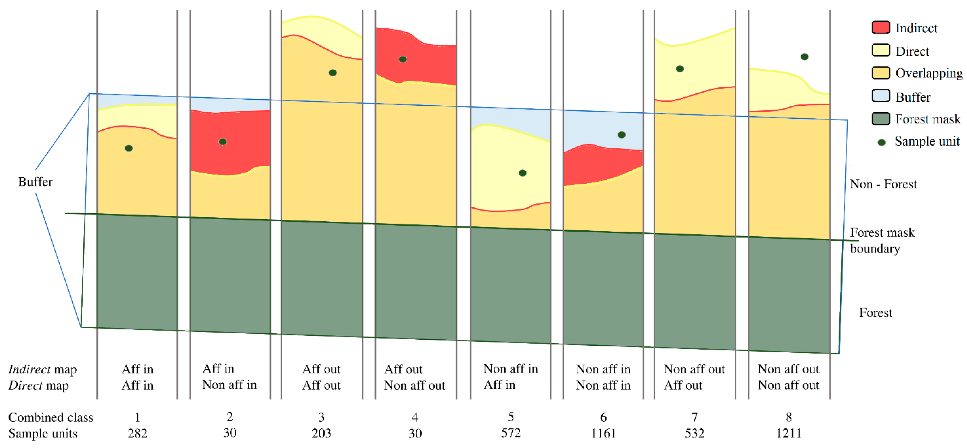
| Map Class | Combination Class | 1 | 2 | 3 | 4 | 5 | 6 | 7 | 8 | ||
|---|---|---|---|---|---|---|---|---|---|---|---|
| Sample Units | 282 | 30 | 203 | 30 | 572 | 1161 | 532 | 1211 | |||
| Indirect map | Afforestation | A | Inside forest buffer | ||||||||
| C | Outside forest buffer | ||||||||||
| Non-afforestation | B | Inside forest buffer | |||||||||
| D | Outside forest buffer | ||||||||||
| Direct map | Afforestation | A | Inside forest buffer | ||||||||
| C | Outside forest buffer | ||||||||||
| Non-afforestation | B | Inside forest buffer | |||||||||
| D | Outside forest buffer | ||||||||||
| Map Class | Validation Data | Sum | |||||
|---|---|---|---|---|---|---|---|
| Afforestation | Non- Afforestation | ||||||
| Afforestation inside buffer | |||||||
| Afforestation outside buffer | |||||||
| Non-afforestation inside buffer | |||||||
| Non-afforestation outside buffer | |||||||
| Combination classes | Validation Data | Sum | ||||||
|---|---|---|---|---|---|---|---|---|
| Indirect | Direct | Afforestation | Non- Afforestation | |||||
| Afforestation inside buffer | Afforestation inside buffer | |||||||
| Afforestation inside buffer | Non-afforestation inside buffer | |||||||
| Afforestation outside buffer | Afforestation outside buffer | |||||||
| Afforestation outside buffer | Non-afforestation outside buffer | |||||||
| Non-afforestation inside buffer | Afforestation inside buffer | |||||||
| Non-afforestation inside buffer | Non-afforestation inside buffer | |||||||
| Non-afforestation outside buffer | Afforestation outside buffer | |||||||
| Non-afforestation outside buffer | Non-afforestation outside buffer | |||||||
| Maps Classes Combination | Validation Data | Sum | Class Accuracy | |||||||
|---|---|---|---|---|---|---|---|---|---|---|
| Indirect | Direct | Afforestation | Non- Afforestation | |||||||
| Afforestation inside buffer | Afforestation inside buffer | |||||||||
| Afforestation inside buffer | Non-afforestation inside buffer | |||||||||
| Afforestation inside buffer | #3 | |||||||||
| Afforestation outside buffer | Afforestation outside buffer | |||||||||
| Afforestation outside buffer | Non-afforestation outside buffer | |||||||||
| Afforestation outside buffer | #3 | |||||||||
| Non-afforestation inside buffer | Afforestation inside buffer | |||||||||
| Non-afforestation inside buffer | Non-afforestation inside buffer | |||||||||
| Non-afforestation inside buffer | #3 | |||||||||
| Non-afforestation outside buffer | Afforestation outside buffer | |||||||||
| Non-afforestation outside buffer | Non-afforestation outside buffer | |||||||||
| Non-afforestation outside buffer | #3 | |||||||||
Disclaimer/Publisher’s Note: The statements, opinions and data contained in all publications are solely those of the individual author(s) and contributor(s) and not of MDPI and/or the editor(s). MDPI and/or the editor(s) disclaim responsibility for any injury to people or property resulting from any ideas, methods, instructions or products referred to in the content. |
© 2023 by the authors. Licensee MDPI, Basel, Switzerland. This article is an open access article distributed under the terms and conditions of the Creative Commons Attribution (CC BY) license (https://creativecommons.org/licenses/by/4.0/).
Share and Cite
Francini, S.; Cavalli, A.; D’Amico, G.; McRoberts, R.E.; Maesano, M.; Munafò, M.; Scarascia Mugnozza, G.; Chirici, G. Reusing Remote Sensing-Based Validation Data: Comparing Direct and Indirect Approaches for Afforestation Monitoring. Remote Sens. 2023, 15, 1638. https://doi.org/10.3390/rs15061638
Francini S, Cavalli A, D’Amico G, McRoberts RE, Maesano M, Munafò M, Scarascia Mugnozza G, Chirici G. Reusing Remote Sensing-Based Validation Data: Comparing Direct and Indirect Approaches for Afforestation Monitoring. Remote Sensing. 2023; 15(6):1638. https://doi.org/10.3390/rs15061638
Chicago/Turabian StyleFrancini, Saverio, Alice Cavalli, Giovanni D’Amico, Ronald E. McRoberts, Mauro Maesano, Michele Munafò, Giuseppe Scarascia Mugnozza, and Gherardo Chirici. 2023. "Reusing Remote Sensing-Based Validation Data: Comparing Direct and Indirect Approaches for Afforestation Monitoring" Remote Sensing 15, no. 6: 1638. https://doi.org/10.3390/rs15061638
APA StyleFrancini, S., Cavalli, A., D’Amico, G., McRoberts, R. E., Maesano, M., Munafò, M., Scarascia Mugnozza, G., & Chirici, G. (2023). Reusing Remote Sensing-Based Validation Data: Comparing Direct and Indirect Approaches for Afforestation Monitoring. Remote Sensing, 15(6), 1638. https://doi.org/10.3390/rs15061638