Article

A New Strategy for Individual Tree Detection and Segmentation from Leaf-on and Leaf-off UAV-LiDAR Point Clouds Based on Automatic Detection of Seed Points

1
Department of Ecology, Nanjing Forestry University, Nanjing 210037, China
2
Department of Geography and Planning, University of Saskatchewan, 117 Science Place, Saskatoon, SK S7N5C8, Canada
3
Co-Innovation Center for Sustainable Forestry in Southern China, Nanjing Forestry University, Nanjing 210037, China
*
Author to whom correspondence should be addressed.
Remote Sens. 2023, 15(6), 1619; https://doi.org/10.3390/rs15061619
Submission received: 31 January 2023 / Revised: 15 March 2023 / Accepted: 15 March 2023 / Published: 16 March 2023
(This article belongs to the Collection Feature Paper Special Issue on Forest Remote Sensing)

Abstract

:
Accurate and efficient estimation of forest volume or biomass is critical for carbon cycles, forest management, and the timber industry. Individual tree detection and segmentation (ITDS) is the first and key step to ensure the accurate extraction of detailed forest structure parameters from LiDAR (light detection and ranging). However, ITDS is still a challenge to achieve using UAV-LiDAR (LiDAR from Unmanned Aerial Vehicles) in broadleaved forests due to the irregular and overlapped canopies. We developed an efficient and accurate ITDS framework for broadleaved forests based on UAV-LiDAR point clouds. It involves ITD (individual tree detection) from point clouds taken during the leaf-off season, initial ITS (individual tree segmentation) based on the seed points from ITD, and improvement of initial ITS through a refining process. The results indicate that this new proposed strategy efficiently provides accurate results for ITDS. We show the following: (1) point-cloud-based ITD methods, especially the Mean Shift, perform better for seed point selection than CHM-based (Canopy Height Model) ITD methods on the point clouds from leaf-off seasons; (2) seed points significantly improved the accuracy and efficiency of ITS algorithms; (3) the refining process using DBSCAN (density-based spatial clustering of applications with noise) and kNN (k-Nearest Neighbor classifier) classification significantly reduced edge errors in ITS results. Our study developed a novel ITDS strategy for UAV-LiDAR point clouds that demonstrates proficiency in dense deciduous broadleaved forests, and this proposed ITDS framework could be applied to single-phase point clouds instead of the multi-temporal LiDAR data in the future if the point clouds have detailed tree trunk points.

Graphical Abstract

1. Introduction

Global forest ecosystems provide ecological, social, and economic benefits by providing numerous ecosystem services including supplying productivity and regulating water and carbon cycles [1]. Accurate assessment of forest volume and biomass is the foundation of the timber industry and forest management [2,3,4,5]. Remote sensing approaches, through non-destructive monitoring, are widely applied in forest research for volume and biomass estimation in a range of spatial and temporal scales [6]. The current wide application of light detection and ranging (LiDAR) sensors in forest research advances the quantification of three-dimensional (3D) forests, as the collected 3D point clouds are able to directly capture the 3D information of forests [7], improving the estimation accuracy of forest volume and biomass [7,8]. LiDAR is able to retrieve detailed forest structures parameters including tree height [9], crown diameter [10], crown projected area [10], basal area [11], stand density [12], canopy volume [13], canopy cover [14], diameter at breast height (DBH) [15], stem volume [5], tree species [16], and biomass [17]. UAV-LiDAR (LiDAR taken from unmanned aerial vehicles) improves flexibility and has higher point density and lower cost compared to airborne LiDAR [14,18,19,20], adding information to the quantification of forest structure, volume, and biomass to the individual tree scale [19,21]. This adds considerable information to conventional forest inventory at the individual tree level. For either airborne LiDAR or UAV-LiDAR, individual tree detection and segmentation (ITDS) is a key step to ensure the accurate estimation of single tree structural attributes, volume, and biomass [22,23,24].
Two methodological categories, CHM-based (Canopy Height Model) and point-cloud-based, are commonly applied to UAV-LiDAR data for single tree detection and segmentation [24,25]. Although both CHM-based and point-cloud-based methods have satisfied accuracy for ITDS from UAV-LiDAR [9,14,26], both have shown much lower accuracy in broadleaved forests with irregular canopies, overlapping canopies, and/or multiple stems [26,27,28,29]. The CHM-based method first applies search windows to find canopy maxima and to identify tree locations using CHM data. Then segmentation algorithms (e.g., watershed and region growing methods) are applied to delineate individual tree crowns [23,30,31,32,33,34,35]. CHM-based methods significantly improved the accuracy for ITDS when it was first constructed for airborne LiDAR data [36]. However, high commission or omission errors for individual tree detection (ITD) from CHM brings bias into individual tree segmentation (ITS) for broadleaved forests, especially in forests with complex and overlapping crown structures [19,37,38]. To improve the accuracy of CHM-based methods for single tree segmentation and detection, previous studies have applied marker-based watershed algorithms [29,39]. However, most of these methods require human intervention for marker selection and threshold setting [38], limiting the use of automatic, batch processing.
Unlike CHM-based methods, the point-cloud-based method applies cluster algorithms (e.g., Kmeans clusters) based on point clouds for searching 3D clusters as individual tree segmentation [19,26,40]. Theoretically, point-cloud-based methods have higher accuracy for ITDS, but require more computation time [41] comparing to CHM. Most of the point-cloud-based methods require algorithms for seed point selections [42,43]. Trunk points located at the base of trees were often selected as seed points for bottom-up ITS, which has been proven to be more accurate than up-bottom segmentation especially in broadleaved forests [28,44,45]. However, due to the high canopy cover in the growing season of deciduous broadleaved forests or evergreen broadleaved forests, it is difficult to extract a seed point from the bottom of the tree in this application. Various cluster algorithms have been tested for ITS, including region growing [42], Kmeans [46], mean shift [47,48], normalized cut [19], density-based spatial clustering of applications with noise (DBSCAN) [49], and deep learning network [43]. Although these clustering algorithms are effective in forests, their effectiveness relies heavily on the accuracy of ITD and thus remains a challenge in broadleaved forests with overlapping tree canopies and similar height and density distributions [7].
Thus, a gap remains for an efficient, accurate, and applicable ITDS method for broadleaved forests. Previous studies have improved the accuracy for extracting forest parameters [16] and classifying tree species [50,51] by merging LiDAR point clouds from leaf-off and leaf-on seasons to extract forest variables or classify forest species. However, few studies have focused on ITDS using multi-temporal UAV-LiDAR data. Since trunk points contribute to improving the accuracy of ITD and bottom-up segmentation methods [28,44,45], it is worthwhile to explore the potential for combining multi-temporal ITDS point clouds in broadleaved forests; point clouds from leaf-off season could capture dense tree trunk points and point clouds from leaf-on season would obtain detailed 3D information of tree canopies.
To address the challenges mentioned by the utilization of UAV-LiDAR data in broadleaved forests and to develop a more efficient, precise, and practical methodology, this study proposed a new ITDS framework based on point clouds from multiple seasons in broadleaved forests. Our specific objectives are as follows: (1) to develop a strategy for automatic ITD from UAV-LiDAR point clouds in leaf-off season; (2) to explore the best ITS strategy based on the seed points from the automatic ITD and UAV-LiDAR point clouds in leaf-on season; and (3) to improve the efficiency and capacity of the developed ITDS framework through a unique refining process.

2. Materials and Methods
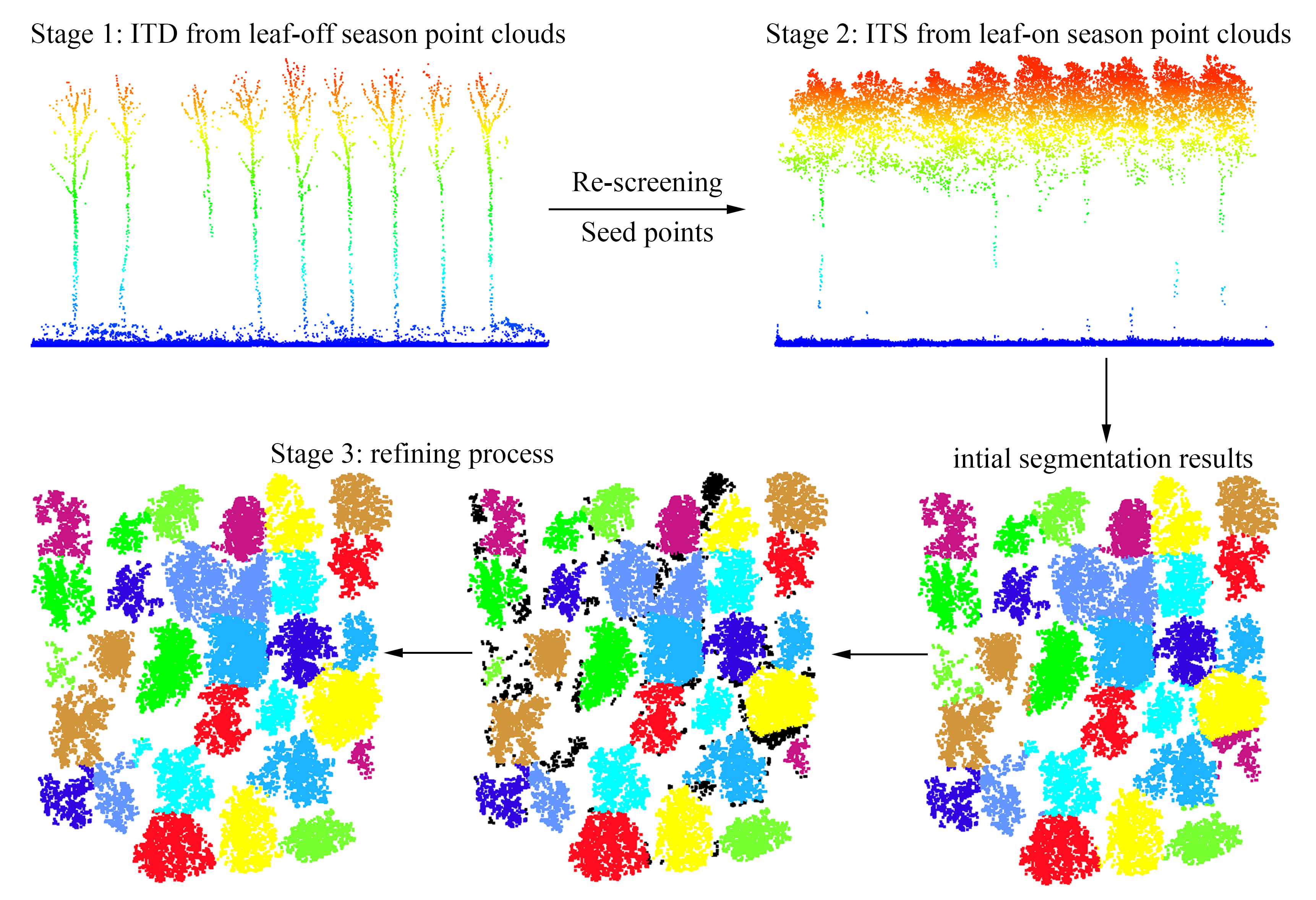
2.1. Study Area

Our research was conducted in a poplar (Populus deltoids) plantation in the eastern part of Dongtai City, Jiangsu Province (120.82°N, 32.87°W, Figure 1). The plantation (stand age 8–20 years) is located in a relatively flat region near the coast with elevation from 11 to 14 m (relatively flat terrain). The annual mean temperature is 15.4 °C and the annual rainfall is 1494 mm [52]. The main soil type is desalinated meadow soil with sandy loam texture [52].

2.2. UAV-LiDAR and Field Data Collection
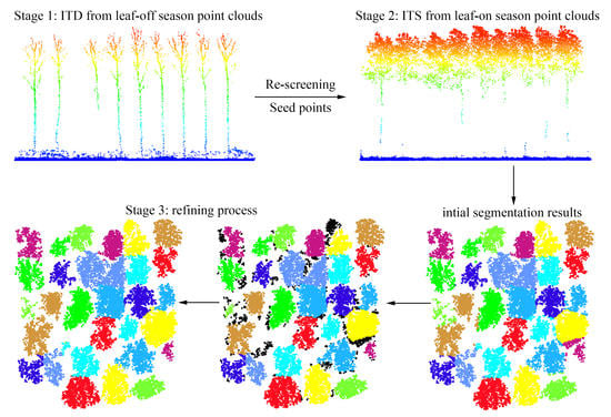
UAV-LiDAR point clouds were collected in both leaf-off and leaf-on seasons (January 2021 and May 2021) using a Velodyne VLP-16 LiDAR sensor (wavelength: 903 nm) carried by a six-rotor DJI M600 PRO UAV (Figure 2). This UAV-LiDAR system operates with a pulse repetition frequency of 30 kHZ and a vertical scanning angle of ±15° and horizontal scanning angle of 360°. The UAV-LiDAR data for this study were collected with the flight altitude of 70 m, flight speed of 3.6 m·s−1, flight interval of 60 m, and horizontal scanning angle of ±70°. We also recorded the point cloud densities in the above-ground part (higher than 2 m; Table 1).
Fieldwork was conducted in January 2021, simultaneous with UAV-LiDAR collection in leaf-off season. We established 12 sample plots in different stand ages with varying planting spacing, tree height, and canopy structural characteristics (Table 1). In each sample plot, we recorded the position of each tree based on four points: north, south, east, and west around the tree base (Figure 1d). The center point of each tree was calculated by the mean center of these four points (Figure 1d) and the number of reference trees in each sample plot (Table 1) was used as the reference tree position for ITD of UAV-LiDAR point clouds (Figure 1c). Due to planned and unplanned deforestation (forestry and wind) during the two data collection periods, we updated the number of reference trees during the fieldwork in May (Table 1).

2.3. Methodology

After the pre-processing of the UAV-LiDAR point cloud data, CHM and normalized point clouds were generated (Section 2.3.1). Then, the accuracy of ITD and the seed point selection for all three methods (local maxima, local minima, and mean shift algorithm) were evaluated based on CHM or normalized point clouds in the leaf-off season (Section 2.3.2, Figure 3). The method with the highest accuracy was applied to extract two seed point types that could be used for the ITS in the leaf-on season (Section 2.3.3). After re-screening the seed points, three seed-based ITS methods (Seeds + Kmeans, Seeds + Dalponte2016, Seeds + Silva2016) were conducted (Section 2.3.3), comparing four direct ITS methods (Dalponte2016, Li2012, PTrees, LayerStacking). A new segmentation refining method was used to improve the accuracy of crown delineation and ITS in all sample plots (Figure 3).

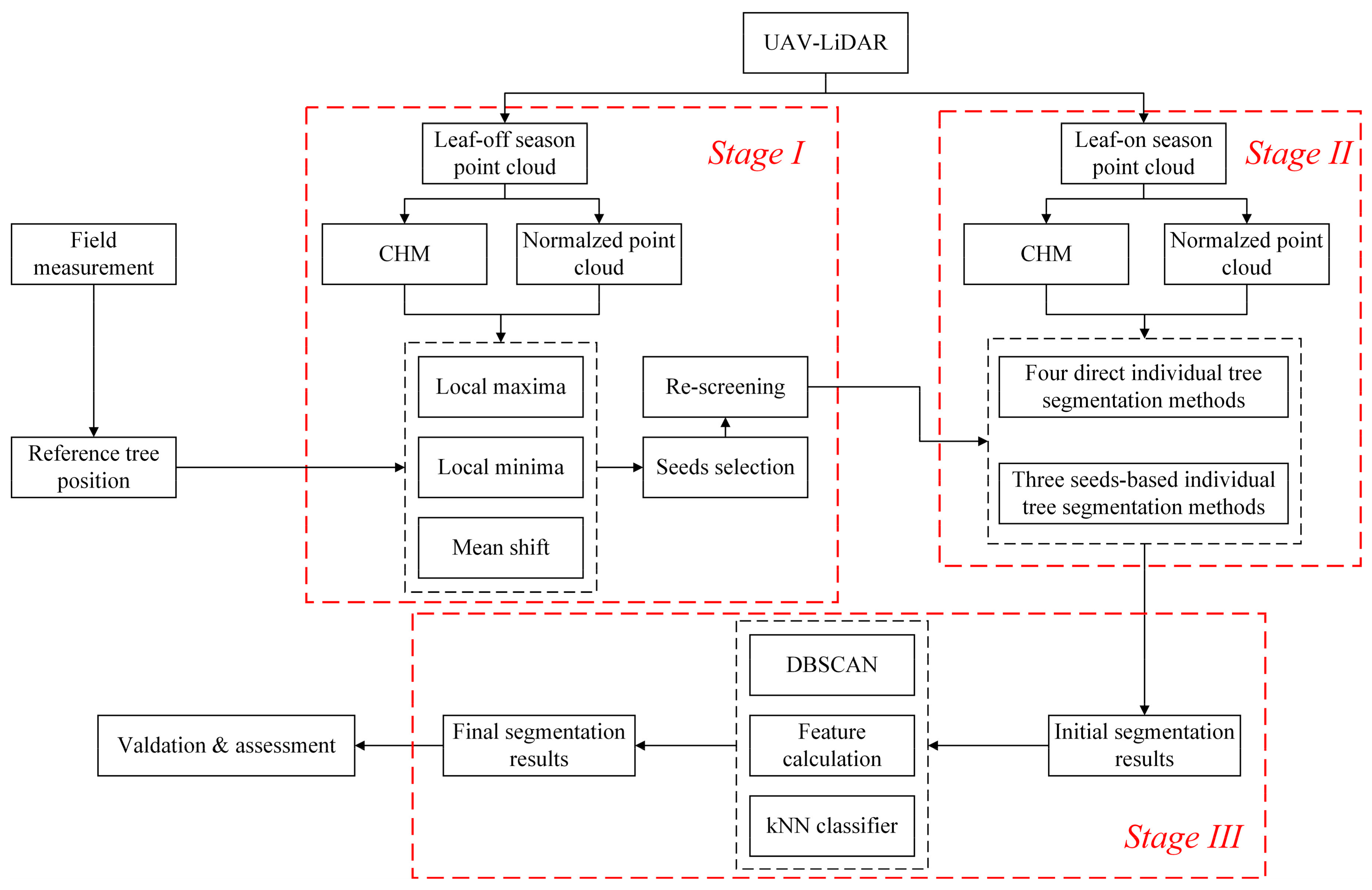
2.3.1. Pre-Processing of UAV-LiDAR Point Cloud Data

The pre-processing steps of UAV-LiDAR point clouds we applied were georeferencing, strip alignment, strip merging, de-noising, and the interpolation. The coordinates of the initial point cloud data were generated based on two systems: real-time-kinematic (RTK) antenna carried on the UAV and paired with the corresponding global positioning system (GPS) base station; and the inertial measurement unit (IMU) in the inertial navigation system (INS) system. All flight strips were merged based on the iterative closest point (ICP) registration algorithm, and the noise points were filtered using the maximum distance from the point to its neighbors. After ground points were classified using an improved progressive triangulated irregular network (TIN) densification filtering algorithm [53], they were interpolated to the digital elevation model (DEM) using the TIN interpolate algorithm. Normalized point cloud data were generated by subtracting the DEM from the de-noised point cloud, which represents the absolute heights of trees and other undergrowth above the elevation. To eliminate spatial error caused by different time phases, we performed a fine registration of the normalized point clouds for leaf-off and leaf-on seasons using the ICP registration algorithm. CHM images with a spatial resolution of 0.1 m were generated from the normalized point clouds based on the grid_canopy function in the lidR package in R software [54].

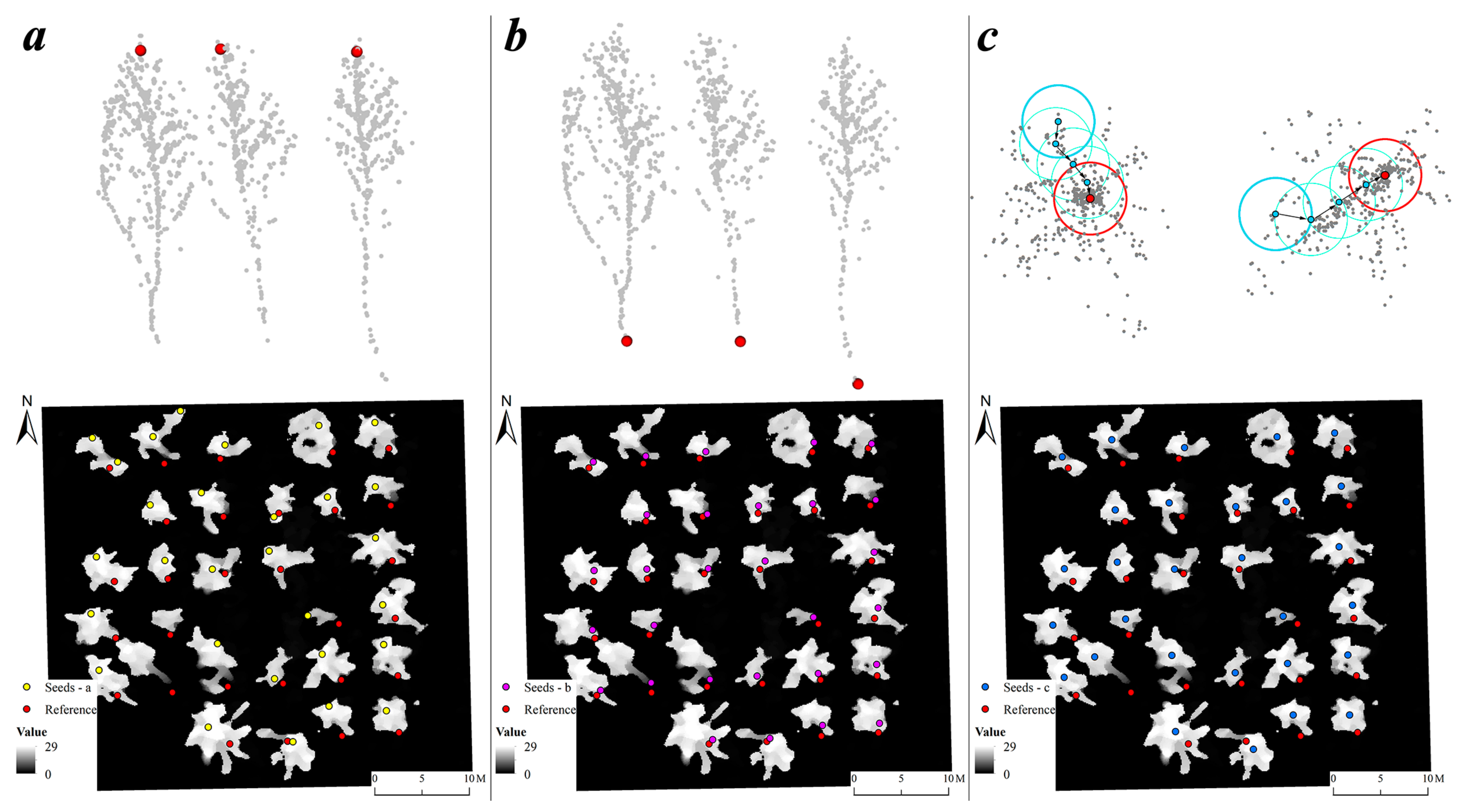
2.3.2. ITD and Seed Points Detection under Leaf-Off Conditions

To extract seeds from UAV-LiDAR data of the leaf-off season, three reliable methods were tested (Figure 4). The first method is commonly applied and uses a local maximum filter algorithm on the CHM images [55]. This method has been shown to have high accuracy for ITD in coniferous forests based on different types of LiDAR data [25]. A median value based on 7 × 7 pixel moving windows was chosen in this study using the focal function in the raster package of R software. Because the CHM image has a spatial resolution of 0.1 m, the actual size of this smoothing window is 0.7 × 0.7 m. The local maximum algorithm was then performed in the smoothed CHM to identify treetops (Figure 4a) based on a fixed circle window. The size of this circle affects the accuracy of ITD, so we tested multiple window sizes adjusted to tree spacing in each plot and selected the size with the best detection performance (Table 2).
The second method is a smoothing window filtering method that is often used to improve ITD accuracy in broadleaved forests [56]. Compared to the first method, this approach searches for the lowest point rather than the treetop for a single tree. This second method is often applied for bottom-up ITS methods, which have been shown to have better ITS performance for broadleaved forests for their potential to eliminate errors caused by complex canopy structure [44]. Specifically, a local minimum filter algorithm was conducted in the normalized point cloud data instead of the CHM image (Figure 4b). Circle window diameters for this second method were the same as those in the first method (Table 2) and both were run in the locate_trees function from lidR package in R software.
The third method is a Mean Shift algorithm, a nonparametric feature-space analysis technique for detecting the local maxima based on a probability density function of the data [57]. Because it was applied by interactively shifting each point in the feature space uphill until it reaches a mode, all the points were classified into a cluster with the same mode. This approach is feasible for directly segmenting point clouds in 3D space [7,47]. The primary parameter for this method is kernel bandwidth, which strongly impacts the cluster results. Instead of adopting this technique on the 3D point cloud directly, we projected the point clouds from the leaf-off season onto the horizontal plane (2D plane) first and then conducted the Mean Shift algorithm from the sklearn.cluster library in Python (Figure 4c). In this way it skips vertical bandwidth selection. Various horizontal bandwidth parameters were tested by trial and error and the best horizontal bandwidth was selected for each plot (Table 2).

2.3.3. ITS in Leaf-On Conditions

To explore the advantage of seed point detection in ITS in UAV-LiDAR point clouds of broadleaved plantations in the leaf-on season, four commonly used ITS methods were compared using the lidR and lidRplugins packages in R software [54]. The first ITS method is an up-bottom segmentation method used by applying a regional growth algorithm on the CHM raster [34]. This first ITS method requires the treetops first be identified from the CHM, which is the same as the local maximum ITD method based on the CHM from the leaf-off season. The diameter of the moving circle window was also determined in the trials using tree spacing in each plot (Table 3). The two important parameters for judging growth for this first ITS method (th_seed and th_cr) were kept as algorithm defaults (0.45 and 0.55) in this study.
The second ITS approach is a regional growth method (an up-bottom), combined with the threshold judgment, based on point cloud data rather than CHM raster [42]. For this second ITS method, the important index that decides which point belongs to which tree is the horizontal Euclidean distance between this point and treetops. Therefore, treetops need to be first selected by a local maximum algorithm based on the normalized point cloud data for this ITS method as well (Table 3). The threshold parameters of dt1 and dt2 were set as algorithm defaults (1.5 and 2).
The third ITS method is PTrees, which is a multi-scale point cloud segmentation algorithm [58]. This method requires the absolute maxima be determined rather than the local maxima. The fundamental principle is to apply a k-nearest neighbor algorithm on the normalized point cloud and calculate the area of a convex hull from these k-nearest points in the 3D space. The primary parameter for this third method is the k; two types of k values (k1, k2) were set to meet multi-scale needs. The k values were selected based on the trials and the point cloud densities for different sample plots (Table 3).
The fourth ITS method, layer stacking, is a segmentation algorithm based on the normalized point cloud data [59]. The principle of this method is to first slice the point clouds according to their heights, obtain the clusters in each layer, and finally locate the position of each tree using the high-density area by overlapping all layers’ results. For this fourth method, the layer thickness was set as default (0.5) and the sizes of two search windows (w1 and w2) were determined by trial for each sample plot (Table 3). We set w1 as 2 × w2 and tested the performance of the algorithm on a scale of w2 (from 1 to 5) and selected the best parameters.
We also designed a segmentation framework based on seed points extracted from the leaf-off poplar plantation (see Section 2.3.2). The specific steps were as follows: (1) re-screening seed points, (2) implementing the segmentation method, and (3) refining segmentation results. The initial seed points were determined with the method with highest accuracy among all three ITD methods based on the LiDAR data from the leaf-off season. To eliminate the error caused by deforestation, a k-nearest neighbor algorithm was applied to evaluate whether each initial seed point is qualified. This is a re-screening of the seed points to match those points calculated from LiDAR data in leaf-off season with that in leaf-on season. The horizontal Euclidean distance between each seed point and its five neighbors in the point cloud from the leaf-on season was calculated first, and then all the distances from the target seed and its neighbors were summed. The sum of the distances was compared with a threshold (1.5 m in this study) to judge whether the specific seed point is valid (Figure 5).
During the second step, three segmentation methods (seed points could be applied to these methods) including Kmeans, region growth, and Voronoi polygon were compared. Kmeans, a common clustering method, determines optimum clusters by continuously iterating center points (iteration times were set to 10 by default). A good starting center point has a strong capacity to achieve good segmentation results from point clouds based on the Kmeans method [46]. We used the center point obtained after clustering with the Mean Shift algorithm (Figure 6a) as the seed point for the Kmeans algorithm. The region growth [34] is an ITS method based on the regional growth of the seed points. Since the initial growth point for this method is the highest location in a specific region, we clustered around the seed points and took those with the highest z-value (where the z-value represents the height of normalized point clouds) in each cluster as the new growth point (Figure 6b). The diameters of the circle moving window in this regional growth method are the same as Dalponte2016 (Table 3). Thus, the segmentation of the Dalpnote2016 algorithm was conducted using accurate seed points which were treetop points extracted by ITD in the leaf-off season.
The third method is to construct a Voronoi polygon directly based on the seed points (the center points) in each sample plot and split the point clouds in a 2D plane with this polygon as reference [60]. We set the max value parameter of a crown diameter (max_cr_factor) at 0.6 in the segmentation using Voronoi polygon, so that the diameter will not exceed 60% of the tree height, which was in line with the characteristics of the forest and could reduce a certain degree of under-segmentation [60]. We located the position difference between the two seed points (center and top) and the reference points by the field RTK (Figure 6c).
After applying these three seed points based ITS methods, individual trees were extracted. However, there were still some errors in the results, especially around tree edges (Figure 7a). To improve accuracy for ITS, the DBSCAN algorithm was applied on the initial individual tree points in the horizontal plane. According to the concept of the DBSCAN algorithm regarding sample point tightness [61], the initial individual tree points were divided into a variety of new point clusters (Figure 7b). Then, three tree-crown features in a horizontal plane—the number of points of the cluster (N), the crown area of the cluster (A), and the crown shape of the cluster (S)—were calculated to evaluate the right cluster for the individual tree. Feature A was measured by the area of the convex hull by applying a convex hull algorithm on each cluster from the initial individual tree points. Feature S was measured by the proportion of the first eigenvalue in all eigenvalues by applying the principal components analysis (PCA) on each cluster of the initial individual tree points (i.e., if the S of one cluster is high, its shape is more likely to be elongated which does not match the actual shape of a tree). We set the condition that the core cluster would be selected as the right tree from the initial tree points by the seed points based ITS method (Equation (1), Figure 7b). The other clusters and the noise points instead of the core cluster are given a new tree label in the 3D space based on the kNN (k-Nearest Neighbor classifier) classification algorithm. An iterative method according to the different values of eps (0.4, 0.55, 0.7) in the DBSCAN method was applied to improve the new segmentation results k from the kNN classification (k value choose 5 points). Each point was identified several times to determine whether to change its tree label. Finally, a result with higher segmentation accuracy was determined (Figure 7c).
T r e e = N i > 0.3 × N A i > 0.3 × A S i = S _ m i n
where T r e e is the core cluster from the initial individual tree points, N i is the number of points of cluster i , A i is the crown area of cluster i ,   S i is the crown shape index of cluster i , N is the total number of the initial individual tree points, A is the total area of all clusters of the initial individual tree points, and S _ m i n is the smallest shape index among all clusters of the initial individual tree points.
To evaluate the improvement of the segmentation results from a data perspective, we manually segmented 15 trees in sample plots of each stand age. Two quantitative indicators were extracted, including the approximate horizontal projected area of the canopy crown (using the product of x and y), and the vertical range of the tree (using the range of z). The results of manual segmentation are compared with segmentation with the refining process and without the refining process based on these two indicators (Figure 8).

2.3.4. Accuracy Evaluation

To evaluate the performance and sensitivity of the proposed ITDS strategy in this study, ITDS results were compared with reference tree locations calculated by the four RTK points at each tree. The numbers of true positives (TP), false negatives (FN), and false positives (FP) were counted. TP is the number of trees detected from UAV-LiDAR data that matches reference trees, FN is the unmatched reference trees (omission error), and FP is the unmatched trees extracted from UAV-LiDAR data (commission error). Based on these three indices (TP, FN and FP), the accuracy of the ITDS methods is evaluated using three indices (r, p and F; Equations (2)–(4)).
r = T P / T P + F N
p = T P / T P + F P
F = 2 r × p / r + p
where r , recall of the results, is the proportion of ground reference trees detected; p , the precision of the results, is the proportion of detected trees that match ground reference trees; and F is an index of the overall accuracy that is calculated with r and p .

3. Results

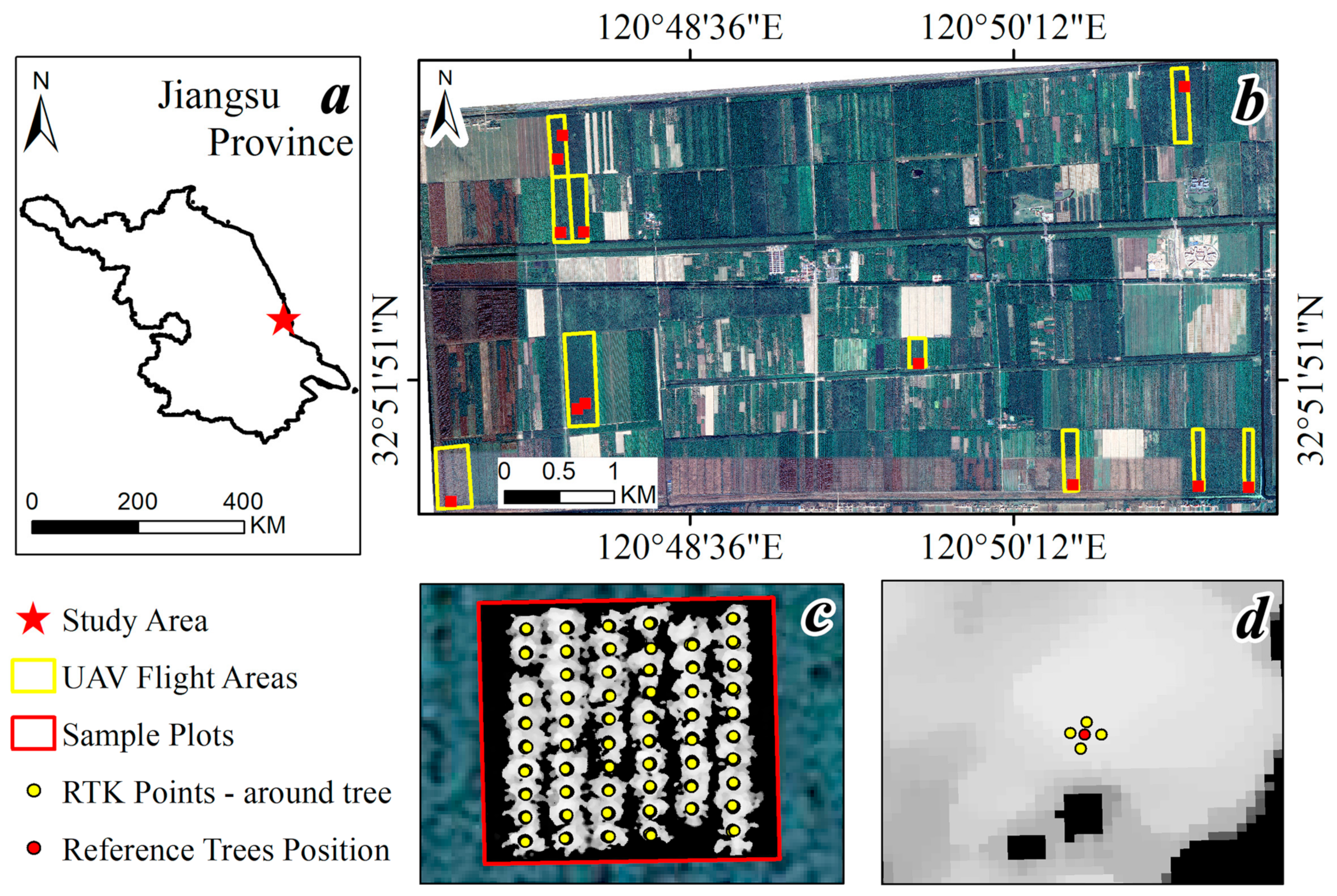
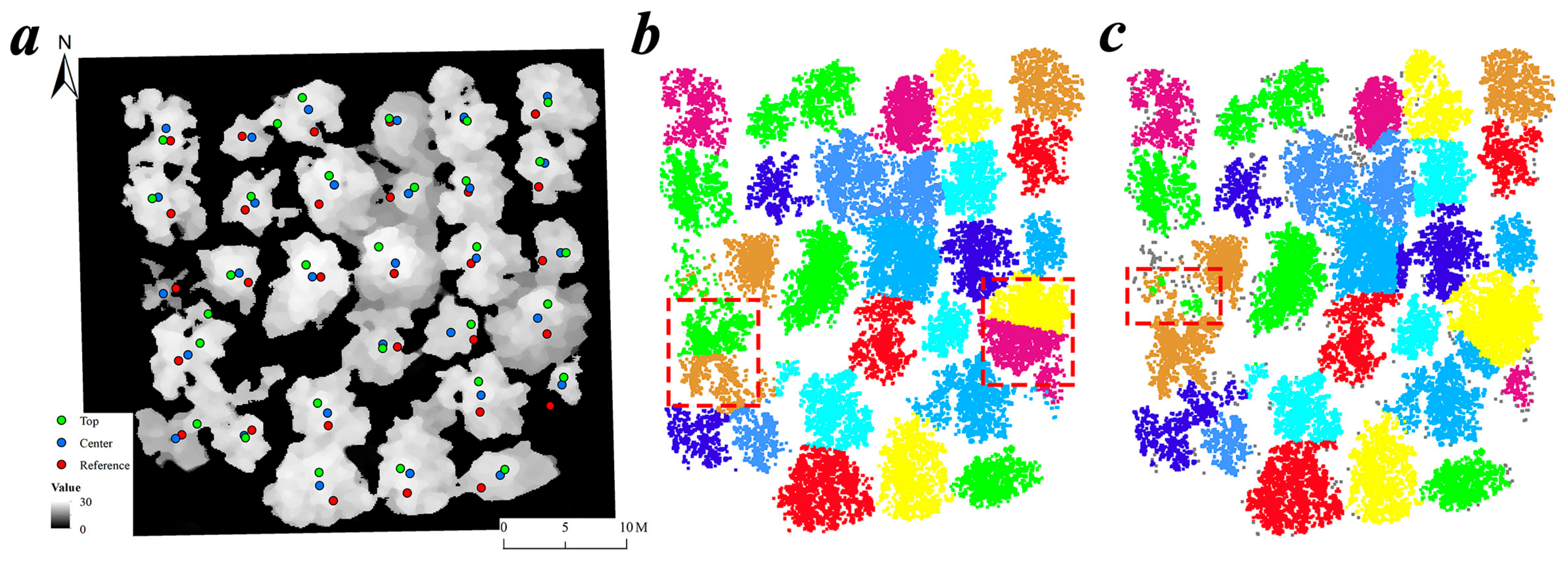
3.1. ITD Results and Seed Points Selection from the UAV-LiDAR Data in Leaf-Off Seasons

Based on the accuracy assessment results for poplar plots among stand ages (Table 4), both Local Minimum-PCD and Mean Shift methods showed better performance for ITD and seed point selection than the Local Maximum-CHM method. Among all the sample plots with six different stand ages, the Local Maximum method had an average detection rate, r, of 0.92, an average accuracy rate, p, of 0.94 and an overall accuracy, F, of 0.93 (Table 4). Compared to the Local Maximum-CHM method, the Local Minimum-PCD and Mean Shift methods have higher accuracy for ITD and seed point selection (i.e., the overall value of r, p, F for both are 0.99; Table 4). Assessing the accuracy of all the plots, the Mean Shift method gave slightly better performance than the Local Minimum-PCD for ITD and seed point selection (except for plots Y14-2 and Y20-3; Table 4).

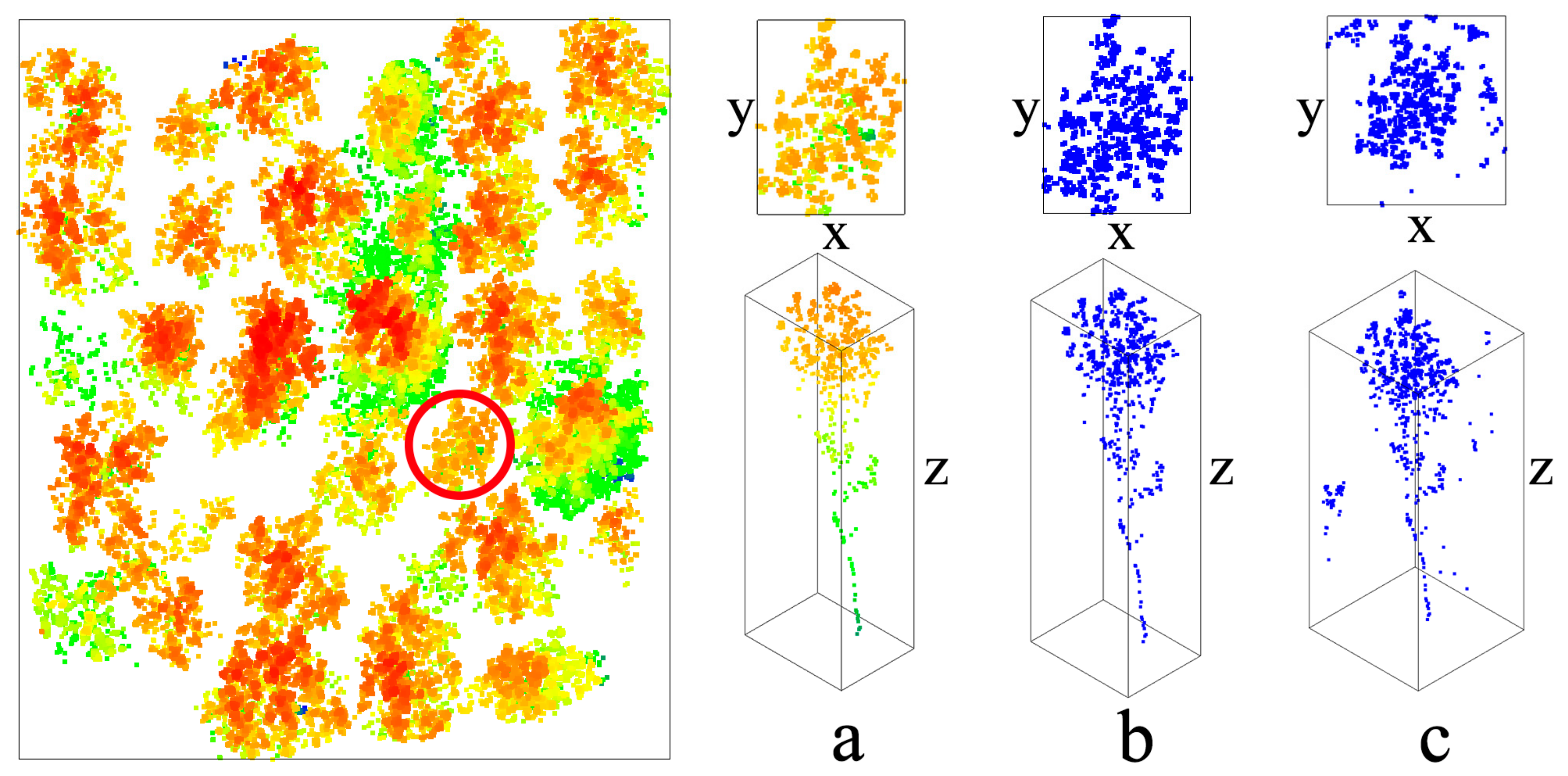
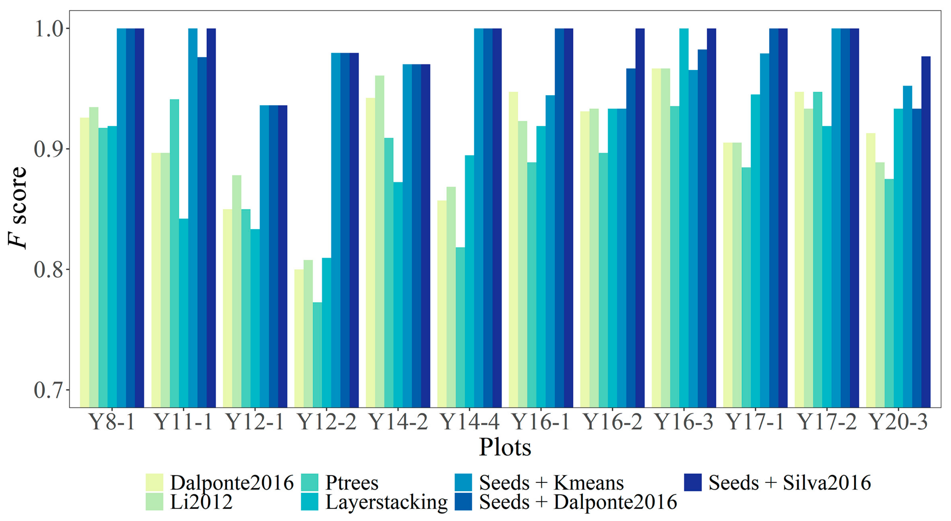
3.2. ITS Results from UAV-LiDAR Points under Leaf-On Conditions

The three seed points based ITS methods (i.e., the seed points based Kmean method: Seeds + Kmeans, the seed points based Dalponte2016 method: Seeds + Dalponte2016, and the seed points based Silva2016 method: Seeds + Silva2016) using seed points extracted during the leaf-off season are more effective than the four ITS methods (Dalponte2016, Li2012, PTrees, LayerStacking) for ITS from UAV-LiDAR data during the leaf-on season (Figure 9 and Table 5). The F score for the three seed points based ITS methods are all stable (i.e., exceeding 0.9; Figure 9). The results of these three seed points based ITS methods are significantly different for the Y16-2 sample plot (F = 1.00, 0.97, and 0.93 for Seeds + Silva2016, Seeds + Dalponte2016, and Seeds + Kmeans, respectively). All three seed points based ITS methods have the same F score in the sample plots of Y8-1, Y12-1, Y12-2, Y14-2, Y14-4, and Y17-2 (Figure 9). In contrast, the F score for the four ITS methods without seed points varied widely among sample plots with significantly low accuracy in the sample plot of Y12-2 (Figure 9). Overall, Seeds + Silva2016 performed best for ITS (418 trees are correctly segmented of a total of 421 trees from the UAV-LiDAR data during leaf-on conditions; Table 5). The Seeds + Silva2016 method also had the highest overall F score (0.99, Table 5), compared to the Seeds + Kmeans and the Seeds + Dalponte2016 methods (0.98, Table 5). For the four ITS methods without seed points, the Dalponte2016 and Li2012 methods performed better (i.e., with the overall F score of 0.91; Table 5) than the other two ITS methods (Table 5).

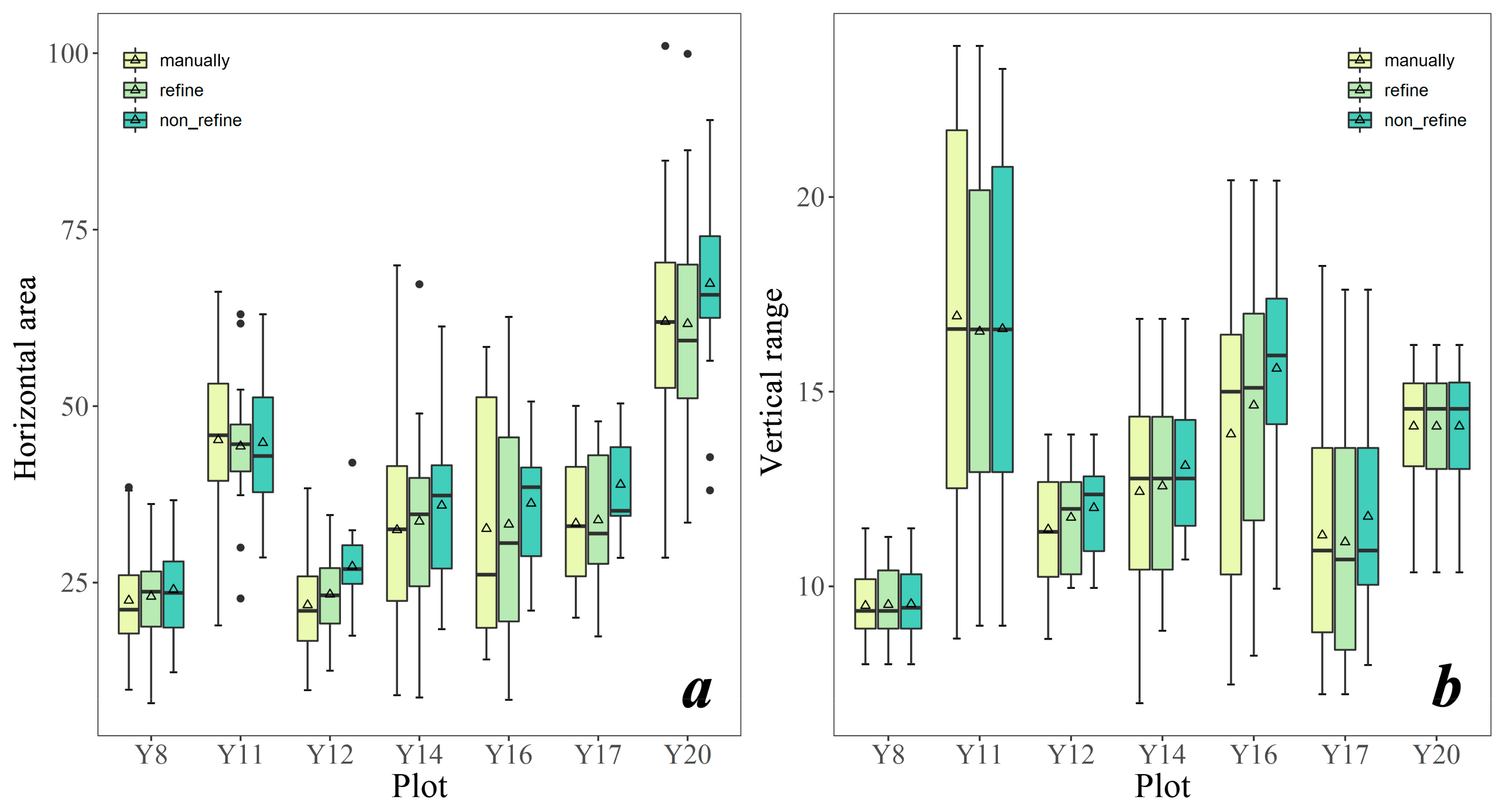
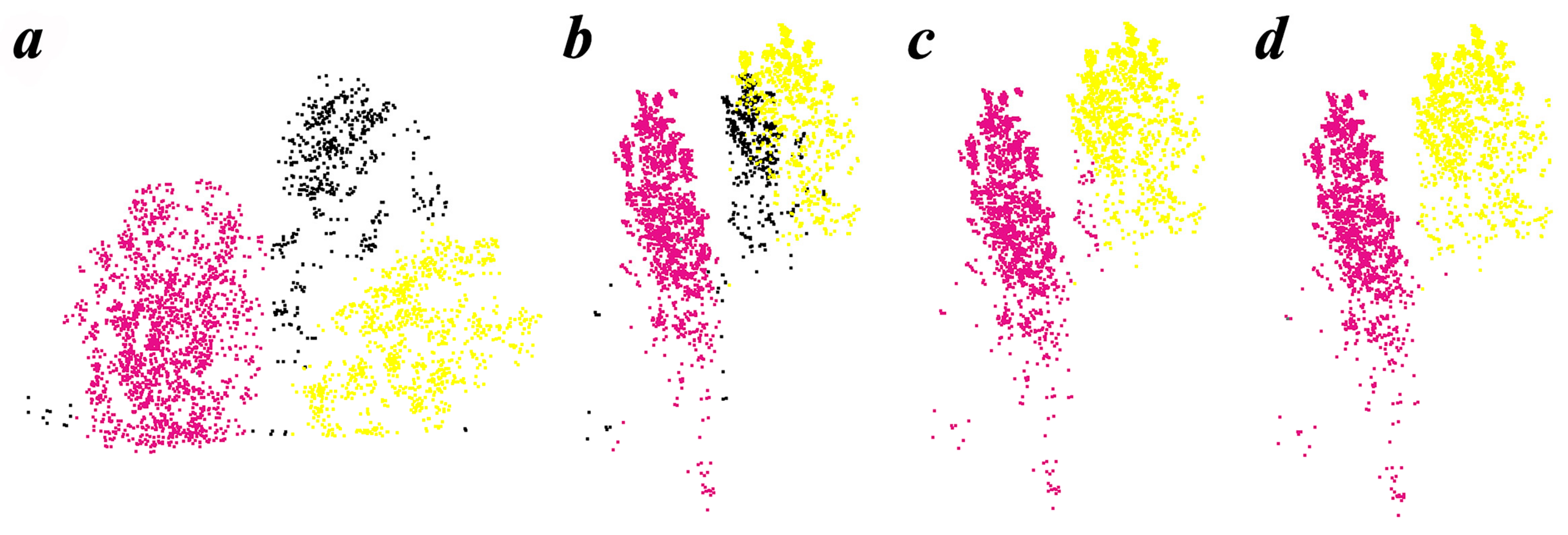
3.3. ITS Results Improvement Based on the Process of Refining

Compared with the difference of the vertical range of individual trees, the difference of the approximate horizontal projected area of the canopy between individual trees of manually and initial segmentation (non_refine result) is larger (Figure 10). Specifically, the initial segmentation result without refining process tends to have a result that is larger than the reference value in both indicators. The process of refining has great improvement on the initial segmentation result on the approximate horizontal projected area of the canopy crown (Figure 10a) and has a slight improvement on the vertical range of the tree extracted (Figure 10b). The mean and median value of these two parameters of each plot will be closer to the manual segmentation result after refining process (Figure 10).

4. Discussion

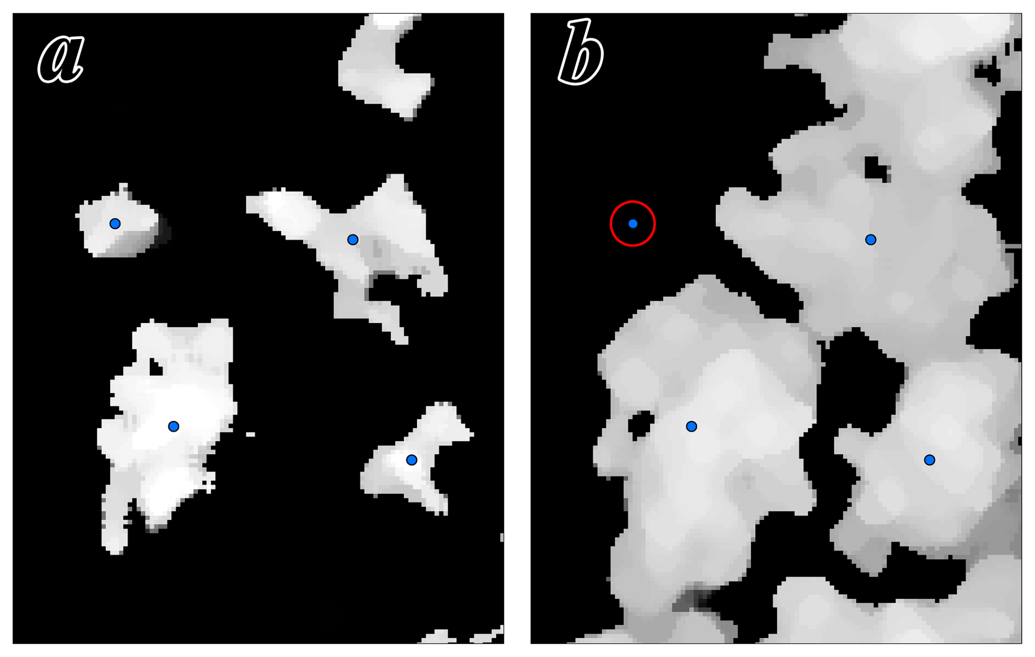
4.1. The Extraction of Seed Points by the ITS Methods

It is difficult to select the optimal threshold for ITDS from LiDAR data in a dense forest, especially when applying these methods to 3D point clouds rather than a CHM raster [41]. However, the identification and segmentation of individual trees during the leaf-off season is relatively easier and the accuracy of ITD is easier to judge. In the leaf-off condition, trunk points and thresholds for the ITD methods are relatively simple to identify using our method.
Although the seed points extracted by Local Minimum have satisfactory accuracy, the Mean Shift method still performs slightly better with the exception of plots Y14-2 and Y20-3. The influence of low trees at Y14-2 and the large branch gap at Y20-3 is responsible for the slight decrease in the performance of the Mean Shift method. We selected the Mean Shift method as the most accurate for seed points selection and ITD because the position of seed points extracted by this algorithm is closer to the tree reference locations (Figure 4). Seed points extracted by the Mean Shift method are more adaptive to the Seeds + Kmeans and Seeds + Silva2016 methods (the two seed points based ITS methods). Although high ITD accuracy is associated with the Local Minimum method (Table 4), the location of its seed points typically deviated from the reference tree locations due to tree tilt.
By conducting the Mean Shift algorithm on point clouds in the 2D plane instead of 3D space in our study, we reduced computational complexity. This speeds the process of Mean Shift algorithm. The connectivity of some individual tree trunk points was poor even under leaf-off conditions (examples in Figure 6b), which may have greatly affected the accuracy of applying this algorithm on point clouds in 3D space [47]. If the Mean Shift method was directly adopted in the 3D space, a great number of clusters would be generated, with its own challenges and errors for ITD and seed points selection. It is for this reason that we applied the DBSCAN algorithm on the point clouds in the 2D plane during the refining process (Section 2.3.3).
We used a moving circular window of fixed size to extract tree top and tree bottom points. Other studies have shown that an adaptive size moving window (typically implemented by functions of tree height and window size) would perform better for ITD [62]. Due to the similar tree heights among sample plots in our study area, we did not explore an adaptive size moving window. It is also worth noting that we did not investigate an adaptive bandwidth size for the Mean Shift algorithm, which avoids parameter selection problems due to different crown widths [63]. The similar canopy size of plantation trees and clear spacing between crowns in the leaf-off season made it easy to select different bandwidths in each sample plot in our study.
Although we developed this ITS framework based on point clouds during both leaf-on and leaf-off seasons, it is also promising to apply this framework to LiDAR data in a single time phase with high density and connectivity of tree trunk point clouds. With the development of UAV-LiDAR systems, several high-frequency LiDAR sensors have tremendous capacity to detect tree trunks in deciduous forests during the leaf-on season [44]. There are many algorithms for forest tree trunk extraction [64,65], which suggest a new direction for trunk-based seed points extraction in our research.

4.2. ITS Methods with or without Seed Points

Among all seven ITS methods we explored, the results of PTrees have the lowest accuracy (Table 5), which appears to be due them relying on the kNN algorithm which is sensitive to point cloud density [58]. Due to the unified point cloud density of all sample plots calculated using a thinning algorithm, the parameters of the PTrees method are difficult to set, resulting in poor ITS performance. We found a large difference among the four direct ITS and three seed points based ITS methods in sample plot Y12-2 (Figure 9). We attribute this to the accuracy of direct ITS methods clearly decreasing in dense forests or forest plantations with similar tree heights (the planting spacing of the sample plot Y12-2 is small; Table 1). However, in this situation, the accuracy of the three seed points based ITS methods remains stable (Figure 9). The low accuracy of the four direct ITS methods in the sample plot Y12-2 may also be due to small trees (low poplars with small crowns) beside larger individuals causing omission errors. It is worth noting that although Y12-1 also has the same low planting spacing, its segmentation is relatively high as the number of surviving trees in this plot is small (Table 1).
The spatial resolution of CHM and the degree of CHM smoothing affect seed point extraction and ITS results [66]. CHM with higher spatial resolution tends to have better results [66], which is an advantage with UAV-LiDAR data because of its significantly higher point density compared to airborne LiDAR. The re-screening process has little effect on results because the difference in the number of trees between the two seasons is small (Table 1). In addition, re-screening is not needed when applying this ITDS framework on the UAV-LiDAR data from a single time phase or among seasons without new plantations or harvested trees.
In addition to error sources from seed point selection point clouds during the leaf-off season with the seed points based ITS methods, the errors in the Seeds + Kmeans method also arose from iterating the central points. The purpose of the iterative process is to better identify cluster centers, but the center points of some small individual trees in the sample plot could move it to the wrong position (Figure 11b). For the Seeds + Dalpnote2016 method, two main error sources exist. First, the treetops of Mean Shift clusters during the leaf-off season are sometimes extracted in the wrong position (i.e., errors from the ITD process under leaf-off position), because of the branches from neighboring trees (Figure 11c). Second, the process of CHM interpolation can also incur errors, and treetop positions can differ between the leaf-on and leaf-off seasons (Figure 11c). The greatest problem for the Seeds + Silva2016 method is segmentation of crown edges (Figure 7a). This is because it is based on the Voronoi polygon that depends solely on Euclidean distance [60]. These errors for the three seed points based ITS methods were highly reduced in the refining process, but could not be totally eliminated for individual trees with high point cloud connectivity [66]. If the crowns of two neighboring trees overlap substantially, the refining process has limited effectiveness. However, we were unable to test the application of our methods in forests with more complex vertical structures in this study, as it may be difficult to accurately segment individual trees that grow under a dense forest canopy. The extraction of these parameters typically requires more advanced techniques [48].
For the evaluation parameters result of the process of refining, it is noticeable that these two parameters tend to have a bigger value in Y11 plot (Figure 10), which may be due to the highest planting spacing in this plantation (Table 1). Because the larger space between trees reduces the overlapping canopy, the extracted horizontal projection area is increased. It also increases the likelihood that the point cloud will detect the tree trunk below the canopy, thus increasing the vertical range. The parameter eps in DBSCAN has some impact on the final results of ITS during the refining process. This parameter was not set to a fixed value for all data due to variation in point cloud density among sample plots. Our method iterates different eps values to improve the capacity of the refining process (Figure 12). The size and interval of eps among iterations could be adjusted, although the preset eps values (0.4, 0.55, 0.7) can essentially meet the refining process in all plots. In addition, the coefficient of N i and A i for the core cluster of initial individual tree points selection (Equation (1)) were derived by trial and error. Specifically, after conducting multiple experiments with coefficients ranging from 0.2 to 0.8, we selected a value of 0.3 based on a comprehensive visual analysis of the sampling sites. This selected coefficient was then uniformly applied to all point cloud data. In theory, it is possible to adjust this parameter individually for each site based on the initial segmentation outcomes. However, it is generally recommended to choose smaller coefficients, as larger ones may lead to under-segmentation errors by reducing the detection rate of the initial tree. In the process of relabeling point clouds for non-core clustering, it was observed that when the value of k is small (less than 10), the value of k seems to have little effect on the resulting classification results; but when k is taken too large, it will increase the possibility of misclassification. Therefore, in this study, the default value of k has been selected as 5 for the sake of consistency and practicality; more details of k value selection can be found in Supplementary Materials A.
The whole processing time of the ITS methods based on 3D point clouds is significantly higher than that based on CHM raster or point clouds in 2D plane (Table 6). Indeed, the processing time of ITS methods based on 3D point clouds increases along with the increasing of point cloud density because they are more sensitive to point cloud density. Therefore, the commonly used ITS methods based on 3D point clouds from airborne LiDAR need to be adjusted when applied to UAV-LiDAR point clouds with much higher density. Voxelization, or down-sampling of 3D point clouds, is one approach to reduce the processing time in this situation [43]. The proposed ITDS framework we used suggests that the seed points based ITS methods significantly reduced the processing time of the direct ITS methods based on 3D point clouds (Table 6). This improves our ability to apply the method on point clouds with high density or large regions in future studies.

5. Conclusions

In conclusion, in this study we developed a new ITDS strategy to effectively use UAV-LiDAR point clouds in dense deciduous broadleaved forests. Seed points were extracted by the Mean Shift method based on the leaf-off season point clouds, obtaining an initial ITS result based on those points and the Voronoi polygon (Silva2016) from the leaf-on point clouds. The initial ITS results were then re-segmented to improve accuracy by a DBSCAN and kNN classification refining process. We find it promising that this method can be applied to single-phase point clouds (i.e., if the data capture enough trunk points) with improvements in UAV-LiDAR surveys—the higher density and higher echo point clouds may better describe forest trunk points. Our detailed conclusions are as follows: (1) the two point-cloud-based ITD methods (the Local Minimum (r = 0.99, p = 0.99, F = 0.99) and Mean Shift methods (r = 0.99, p = 0.99, F = 0.99)) perform better for seed selection and ITD from the LiDAR data during the leaf-off season than the CHM-based ITD method (Local Maximum (r = 0.92, p = 0.94, F = 0.93). (2) The Mean Shift method performs slightly better in different sample plots, because the position of seed points is closer to the reference location of trees. (3) Compared to the four direct ITS methods (Dalponte2016: F = 0.91, Li2012: F = 0.91, PTrees: F = 0.88, LayerStacking: F = 0.90), the three seed points (obtained from ITD results using the Mean Shift method on the UAV-LiDAR data of the leaf-off season) based ITS methods (Seeds + Kmeans: F = 0.98, Seeds + Dalponte2016: F = 0.98, Seeds + Silva2016: F = 0.99) have significantly greater capacity for ITS from UAV-LiDAR data in leaf-on seasons. (4) The Seeds + Silva2016 method achieves the highest overall accuracy because its segmentation results are more stable based on seed points and better in plantations with uniform crown sizes. (5) The refining process of DBSCAN and kNN classification algorithms significantly mitigates edge errors and improves the ITS accuracy. (6) The ITDS framework proposed in this study has an operation time advantage (median processing time of the three seed points based ITS methods are all less than 5 s), which enhances its capacity to be applied on larger regions or more complex forests using high-density UAV-LiDAR point clouds.

Supplementary Materials

The following supporting information can be downloaded at: https://www.mdpi.com/article/10.3390/rs15061619/s1, Supplementary Materials A: The explanation of k value selection for KNN; python script; R script.

Author Contributions

Conceptualization, D.X.; methodology, Y.P.; validation, Y.P. and H.W.; formal analysis, Y.P.; investigation, Y.P., H.W., and X.L.; resources, D.X.; data curation, X.X.; writing—original draft preparation, Y.P.; writing—review and editing, D.X.; visualization, Y.P., H.W., and X.L.; supervision, D.X.; project administration, D.X. and X.X.; funding acquisition, D.X. and X.X. All authors have read and agreed to the published version of the manuscript.

Funding

This research was funded by the National Natural Science Foundation of China (41901361), the Six Talent Peaks Project in Jiangsu Province (TD-XYDXX-006), and the Natural Science Foundation of Jiangsu Province (BK20180769).

Data Availability Statement

Not applicable.

Acknowledgments

The authors would like to acknowledge the field crew for collecting the field data.

Conflicts of Interest

The authors declare no conflict of interest.

References

  1. Hyyppa, J.; Yu, X.; Hyyppa, H.; Vastaranta, M.; Holopainen, M.; Kukko, A.; Kaartinen, H.; Jaakkola, A.; Vaaja, M.; Koskinen, J.; et al. Advances in forest inventory using airborne laser scanning. Remote Sens. 2012, 4, 1190–1207. [Google Scholar] [CrossRef] [Green Version]
  2. Hofstad, O. Review of biomass and volume functions for individual trees and shrubs in southeast Africa. J. Trop. For. Sci. 2005, 17, 151–162. [Google Scholar]
  3. Parresol, B.R. Assessing tree and stand biomass: A review with examples and critical comparisons. For. Sci. 1999, 45, 573–593. [Google Scholar]
  4. Shrestha, D.B.; Sharma, R.P.; Bhandari, S.K. Individual tree aboveground biomass for Castanopsis indica in the mid-hills of Nepal. Agrofor. Syst. 2018, 92, 1611–1623. [Google Scholar] [CrossRef]
  5. Ozcelik, R.; Eraslan, T. Two-stage sampling to estimate individual tree biomass. Turk. J. Agric. For. 2012, 36, 389–398. [Google Scholar]
  6. Chander, G.; Haque, M.O.; Micijevic, E.; Barsi, J.A. A procedure for radiometric recalibration of Landsat 5 TM reflective-band data. IEEE Trans. Geosci. Remote Sens. 2010, 48, 556–574. [Google Scholar] [CrossRef]
  7. Dai, W.; Yang, B.; Dong, Z.; Shaker, A. A new method for 3D individual tree extraction using multispectral airborne LiDAR point clouds. ISPRS J. Photogramm. Remote Sens. 2018, 144, 400–411. [Google Scholar] [CrossRef]
  8. Cao, L.; Liu, H.; Fu, X.; Zhang, Z.; Shen, X.; Ruan, H. Comparison of UAV LiDAR and digital aerial photogrammetry point clouds for estimating forest structural attributes in subtropical planted forests. Forests 2019, 10, 145. [Google Scholar] [CrossRef] [Green Version]
  9. Dalla Corte, A.P.; Souza, D.V.; Rex, F.E.; Sanquetta, C.R.; Mohan, M.; Silva, C.A.; Zambrano, A.M.A.; Prata, G.; de Almeida, D.R.A.; Trautenmueller, J.W.; et al. Forest inventory with high-density UAV-LiDAR: Machine learning approaches for predicting individual tree attributes. Comput. Electron. Agric. 2020, 179, 105815. [Google Scholar] [CrossRef]
  10. Ghanbari Parmehr, E.; Amati, M. Individual tree canopy parameters estimation using UAV-based photogrammetric and LiDAR point clouds in an urban park. Remote Sens. 2021, 13, 2062. [Google Scholar] [CrossRef]
  11. Drake, J.B.; Knox, R.G.; Dubayah, R.O.; Clark, D.B.; Condit, R.; Blair, J.B.; Hofton, M. Above-ground biomass estimation in closed canopy neotropical forests using lidar remote sensing: Factors affecting the generality of relationships. Glob. Ecol. Biogeogr. 2003, 12, 147–159. [Google Scholar] [CrossRef]
  12. Campbell, M.J.; Dennison, P.E.; Hudak, A.T.; Parham, L.M.; Butler, B.W. Quantifying understory vegetation density using small-footprint airborne lidar. Remote Sens. Environ. 2018, 215, 330–342. [Google Scholar] [CrossRef]
  13. Berk, P.; Stajnko, D.; Belsak, A.; Hocevar, M. Digital evaluation of leaf area of an individual tree canopy in the apple orchard using the LiDAR measurement system. Comput. Electron. Agric. 2020, 169, 105158. [Google Scholar] [CrossRef]
  14. Wu, X.; Shen, X.; Cao, L.; Wang, G.; Cao, F. Assessment of individual tree detection and canopy cover estimation using unmanned aerial vehicle based light detection and ranging (UAV-LiDAR) data in planted forests. Remote Sens. 2019, 11, 908. [Google Scholar] [CrossRef] [Green Version]
  15. Sun, Y.; Jin, X.; Pukkala, T.; Li, F. Predicting individual tree diameter of larch (Larix olgensis) from UAV-LiDAR data using six different algorithms. Remote Sens. 2022, 14, 1125. [Google Scholar] [CrossRef]
  16. Kim, S.; McGaughey, R.J.; Andersen, H.-E.; Schreuder, G. Tree species differentiation using intensity data derived from leaf-on and leaf-off airborne laser scanner data. Remote Sens. Environ. 2009, 113, 1575–1586. [Google Scholar] [CrossRef]
  17. Xu, D.; Wang, H.; Xu, W.; Luan, Z.; Xu, X. Lidar applications to estimate forest biomass at individual tree scale: Opportunities, challenges and future perspectives. Forests 2021, 12, 550. [Google Scholar] [CrossRef]
  18. Beland, M.; Parker, G.; Sparrow, B.; Harding, D.; Chasmer, L.; Phinn, S.; Antonarakis, A.; Strahler, A. On promoting the use of lidar systems in forest ecosystem research. For. Ecol. Manag. 2019, 450, 117484. [Google Scholar] [CrossRef]
  19. Yan, W.; Guan, H.; Cao, L.; Yu, Y.; Gao, S.; Lu, J. An automated hierarchical approach for three-dimensional segmentation of single trees using UAV LiDAR data. Remote Sens. 2018, 10, 1999. [Google Scholar] [CrossRef] [Green Version]
  20. Bazezew, M.N.; Hussin, Y.A.; Kloosterman, E.H. Integrating Airborne LiDAR and Terrestrial Laser Scanner forest parameters for accurate above-ground biomass/carbon estimation in Ayer Hitam tropical forest, Malaysia. Int. J. Appl. Earth Obs. Geoinf. 2018, 73, 638–652. [Google Scholar] [CrossRef]
  21. Lu, J.; Wang, H.; Qin, S.; Cao, L.; Pu, R.; Li, G.; Sun, J. Estimation of aboveground biomass of Robinia pseudoacacia forest in the Yellow River Delta based on UAV and Backpack LiDAR point clouds. Int. J. Appl. Earth Obs. Geoinf. 2020, 86, 102014. [Google Scholar] [CrossRef]
  22. White, J.C.; Coops, N.C.; Wulder, M.A.; Vastaranta, M.; Hilker, T.; Tompalski, P. Remote sensing technologies for enhancing forest inventories: A review. Can. J. Remote Sens. 2016, 42, 619–641. [Google Scholar] [CrossRef] [Green Version]
  23. Allouis, T.; Durrieu, S.; Vega, C.; Couteron, P. Stem volume and above-ground biomass estimation of individual pine trees from lidar data: Contribution of full-waveform signals. IEEE J. Sel. Top. Appl. Earth Obs. Remote Sens. 2013, 6, 924–934. [Google Scholar] [CrossRef]
  24. Jaskierniak, D.; Lucieer, A.; Kuczera, G.; Turner, D.; Lane, P.N.J.; Benyon, R.G.; Haydon, S. Individual tree detection and crown delineation from Unmanned Aircraft System (UAS) LiDAR in structurally complex mixed species eucalypt forests. ISPRS J. Photogramm. Remote Sens. 2021, 171, 171–187. [Google Scholar] [CrossRef]
  25. Silva, C.A.; Hudak, A.T.; Vierling, L.A.; Valbuena, R.; Cardil, A.; Mohan, M.; Alves Almeida, D.R.; Broadbent, E.N.; Zambrano, A.M.A.; Wilkinson, B.; et al. Treetop: A shiny-based application and R package for extracting forest information from LiDAR data for ecologists and conservationists. Methods Ecol. Evol. 2022, 13, 1164–1176. [Google Scholar] [CrossRef]
  26. Balsi, M.; Esposito, S.; Fallavollita, P.; Nardinocchi, C. Single-tree detection in high-density lidar data from UAV-based survey. Eur. J. Remote Sens. 2018, 51, 679–692. [Google Scholar] [CrossRef] [Green Version]
  27. Brede, B.; Lau, A.; Bartholomeus, H.M.; Kooistra, L. Comparing RIEGL RiCOPTER UAV LiDAR derived canopy height and DBH with terrestrial LiDAR. Sensors 2017, 17, 2371. [Google Scholar] [CrossRef]
  28. Picos, J.; Bastos, G.; Miguez, D.; Alonso, L.; Armesto, J. Individual tree detection in a eucalyptus plantation using unmanned aerial vehicle (UAV)-LiDAR. Remote Sens. 2020, 12, 885. [Google Scholar] [CrossRef] [Green Version]
  29. Yin, D.; Wang, L. Individual mangrove tree measurement using UAV-based lidar data: Possibilities and challenges. Remote Sens. Environ. 2019, 223, 34–49. [Google Scholar] [CrossRef]
  30. Goldbergs, G.; Levick, S.R.; Lawes, M.; Edwards, A. Hierarchical integration of individual tree and area-based approaches for savanna biomass uncertainty estimation from airborne LiDAR. Remote Sens. Environ. 2018, 205, 141–150. [Google Scholar] [CrossRef]
  31. Anjin, C.; Yongmin, K.; Yongil, K.; Yangdam, E. Estimation of individual tree biomass from airborne LiDAR data using tree height and crown diameter. Disaster Adv. 2012, 5, 360–365. [Google Scholar]
  32. Kim, Y.; Chang, A.; Kim, Y.; Song, J.; Kim, C. Estimation of forest biomass from airborne LiDAR data as measures against Global Warming-Individual Tree Unit and Forest Stand Unit. Disaster Adv. 2012, 5, 295–299. [Google Scholar]
  33. Wallace, L.; Lucieer, A.; Watson, C.S. Evaluating tree detection and segmentation routines on very high resolution UAV LiDAR data. IEEE Trans. Geosci. Remote Sens. 2014, 52, 7619–7628. [Google Scholar] [CrossRef]
  34. Dalponte, M.; Coomes, D.A. Tree-centric mapping of forest carbon density from airborne laser scanning and hyperspectral data. Methods Ecol. Evol. 2016, 7, 1236–1245. [Google Scholar] [CrossRef] [Green Version]
  35. Ma, K.; Chen, Z.; Fu, L.; Tian, W.; Jiang, F.; Yi, J.; Du, Z.; Sun, H. Performance and sensitivity of individual tree segmentation methods for UAV-LiDAR in multiple forest types. Remote Sens. 2022, 14, 298. [Google Scholar] [CrossRef]
  36. Apostol, B.; Lorent, A.; Petrila, M.; Gancz, V.; Badea, O. Height extraction and stand volume estimation based on fusion airborne LiDAR data and terrestrial measurements for a Norway spruce Picea abies (L.) karst. Test site in Romania. Not. Bot. Horti Agrobot. Cluj-Napoca 2016, 44, 313–323. [Google Scholar] [CrossRef] [Green Version]
  37. Zhang, J.; Sohn, G.; Bredif, M. A hybrid framework for single tree detection from airborne laser scanning data: A case study in temperate mature coniferous forests in Ontario, Canada. ISPRS J. Photogramm. Remote Sens. 2014, 98, 44–57. [Google Scholar] [CrossRef] [Green Version]
  38. Dong, T.; Zhou, Q.; Gao, S.; Shen, Y. Automatic detection of single trees in airborne laser scanning data through gradient orientation clustering. Forests 2018, 9, 291. [Google Scholar] [CrossRef] [Green Version]
  39. Ene, L.; Naesset, E.; Gobakken, T. Single tree detection in heterogeneous boreal forests using airborne laser scanning and area-based stem number estimates. Int. J. Remote Sens. 2012, 33, 5171–5193. [Google Scholar] [CrossRef]
  40. Fu, L.; Liu, Q.; Sun, H.; Wang, Q.; Li, Z.; Chen, E.; Pang, Y.; Song, X.; Wang, G. Development of a system of compatible individual tree diameter and aboveground biomass prediction models using error-in-variable regression and airborne LiDAR data. Remote Sens. 2018, 10, 325. [Google Scholar] [CrossRef] [Green Version]
  41. Liu, L.; Lim, S.; Shen, X.; Yebra, M. A hybrid method for segmenting individual trees from airborne LiDAR data. Comput. Electron. Agric. 2019, 163, 104871. [Google Scholar] [CrossRef]
  42. Li, W.; Guo, Q.; Jakubowski, M.K.; Kelly, M. A new method for segmenting individual trees from the lidar point cloud. Photogramm. Eng. Remote Sens. 2012, 78, 75–84. [Google Scholar] [CrossRef] [Green Version]
  43. Luo, H.; Khoshelham, K.; Chen, C.; He, H. Individual tree extraction from urban mobile laser scanning point clouds using deep pointwise direction embedding. ISPRS J. Photogramm. Remote Sens. 2021, 175, 326–339. [Google Scholar] [CrossRef]
  44. Lu, X.; Guo, Q.; Li, W.; Flanagan, J. A bottom-up approach to segment individual deciduous trees using leaf-off lidar point cloud data. ISPRS J. Photogramm. Remote Sens. 2014, 94, 1–12. [Google Scholar] [CrossRef]
  45. Tao, S.; Wu, F.; Guo, Q.; Wang, Y.; Li, W.; Xue, B.; Hu, X.; Li, P.; Tian, D.; Li, C.; et al. Segmenting tree crowns from terrestrial and mobile LiDAR data by exploring ecological theories. ISPRS J. Photogramm. Remote Sens. 2015, 110, 66–76. [Google Scholar] [CrossRef] [Green Version]
  46. Morsdorf, F.; Meier, E.; Allgöwer, B.; Nüesch, D. Clustering in airborne laser scanning raw data for segmentation of single trees. Int. Arch. Photogramm. Remote Sens. Spat. Inf. Sci. 2003, 34, W13. [Google Scholar]
  47. Ferraz, A.; Bretar, F.; Jacquemoud, S.; Goncalves, G.; Pereira, L.; Tome, M.; Soares, P. 3-D mapping of a multi-layered Mediterranean forest using ALS data. Remote Sens. Environ. 2012, 121, 210–223. [Google Scholar] [CrossRef]
  48. Huo, L.; Lindberg, E.; Holmgren, J. Towards low vegetation identification: A new method for tree crown segmentation from LiDAR data based on a symmetrical structure detection algorithm (SSD). Remote Sens. Environ. 2022, 270, 112857. [Google Scholar] [CrossRef]
  49. Zhen, Z.; Yang, L.; Ma, Y.; Wei, Q.; Il Jin, H.; Zhao, Y. Upscaling aboveground biomass of larch (Larix olgensis Henry) plantations from field to satellite measurements: A comparison of individual tree-based and area-based approaches. GIScience Remote Sens. 2022, 59, 722–743. [Google Scholar] [CrossRef]
  50. Hamraz, H.; Jacobs, N.B.; Contreras, M.A.; Clark, C.H. Deep learning for conifer/deciduous classification of airborne LiDAR 3D point clouds representing individual trees. ISPRS J. Photogramm. Remote Sens. 2019, 158, 219–230. [Google Scholar] [CrossRef] [Green Version]
  51. Kaminska, A.; Lisiewicz, M.; Sterenczak, K. Single tree classification using multi-temporal ALS data and CIR imagery in mixed old-growth forest in Poland. Remote Sens. 2021, 13, 5101. [Google Scholar] [CrossRef]
  52. Li, Y.; Chen, Y.; Xu, C.; Xu, H.; Zou, X.; Chen, H.Y.H.; Ruan, H. The abundance and community structure of soil arthropods in reclaimed coastal saline soil of managed poplar plantations. Geoderma 2018, 327, 130–137. [Google Scholar] [CrossRef]
  53. Zhao, X.; Guo, Q.; Su, Y.; Xue, B. Improved progressive tin densification filtering algorithm for airborne LiDAR data in forested areas. ISPRS J. Photogramm. Remote Sens. 2016, 117, 79–91. [Google Scholar] [CrossRef] [Green Version]
  54. Roussel, J.-R.; Auty, D.; Coops, N.C.; Tompalski, P.; Goodbody, T.R.H.; Meador, A.S.; Bourdon, J.-F.; de Boissieu, F.; Achim, A. lidR: An R package for analysis of Airborne Laser Scanning (ALS) data. Remote Sens. Environ. 2020, 251, 112061. [Google Scholar] [CrossRef]
  55. Qi, C.; Baldocchi, D.; Gong, P.; Kelly, M. Isolating individual trees in a savanna woodland using small footprint LiDAR data. Photogramm. Eng. Remote Sens. 2006, 72, 923–932. [Google Scholar]
  56. Nasiri, V.; Darvishsefat, A.A.; Arefi, H.; Pierrot-Deseilligny, M.; Namiranian, M.; Le Bris, A. Unmanned aerial vehicles (UAV)-based canopy height modeling under leaf-on and leaf-off conditions for determining tree height and crown diameter (case study: Hyrcanian mixed forest). Can. J. For. Res. 2021, 51, 962–971. [Google Scholar] [CrossRef]
  57. Cheng, Y. Mean shift, mode seeking, and clustering. IEEE Trans. Pattern Anal. Mach. Intell. 1995, 17, 790–799. [Google Scholar] [CrossRef] [Green Version]
  58. Vega, C.; Hamrouni, A.; El Mokhtari, S.; Morel, J.; Bock, J.; Renaud, J.P.; Bouvier, M.; Durrieu, S. PTrees: A point-based approach to forest tree extraction from LiDAR data. Int. J. Appl. Earth Obs. Geoinf. 2014, 33, 98–108. [Google Scholar] [CrossRef]
  59. Ayrey, E.; Fraver, S.; Kershaw, J.A., Jr.; Kenefic, L.S.; Hayes, D.; Weiskittel, A.R.; Roth, B.E. Layer stacking: A novel algorithm for individual forest tree segmentation from LiDAR point clouds. Can. J. Remote Sens. 2017, 43, 16–27. [Google Scholar] [CrossRef]
  60. Silva, C.A.; Hudak, A.T.; Vierling, L.A.; Loudermilk, E.L.; O’Brien, J.J.; Hiers, J.K.; Jack, S.B.; Gonzalez-Benecke, C.; Lee, H.; Falkowski, M.J.; et al. Imputation of individual longleaf pine (Pinus palustris mill.) tree attributes from field and lidar data. Can. J. Remote Sens. 2016, 42, 554–573. [Google Scholar] [CrossRef]
  61. Fu, H.; Li, H.; Dong, Y.; Xu, F.; Chen, F. Segmenting individual tree from TLS point clouds using improved DBSCAN. Forests 2022, 13, 566. [Google Scholar] [CrossRef]
  62. Young, D.J.N.; Koontz, M.J.; Weeks, J. Optimizing aerial imagery collection and processing parameters for drone-based individual tree mapping in structurally complex conifer forests. Methods Ecol. Evol. 2022, 13, 1447–1463. [Google Scholar] [CrossRef]
  63. Yan, W.; Guan, H.; Cao, L.; Yu, Y.; Li, C.; Lu, J. A self-adaptive mean shift tree-segmentation method using UAV LiDAR data. Remote Sens. 2020, 12, 515. [Google Scholar] [CrossRef] [Green Version]
  64. Ferrara, R.; Virdis, S.G.P.; Ventura, A.; Ghisu, T.; Duce, P.; Pellizzaro, G. An automated approach for wood-leaf separation from terrestrial LiDAR point clouds using the density based clustering algorithm DBSCAN. Agric. For. Meteorol. 2018, 262, 434–444. [Google Scholar] [CrossRef]
  65. Itakura, K.; Miyatani, S.; Hosoi, F. Estimating tree structural parameters via automatic tree segmentation from LiDAR point cloud data. IEEE J. Sel. Top. Appl. Earth Obs. Remote Sens. 2022, 15, 555–564. [Google Scholar] [CrossRef]
  66. Lisiewicz, M.; Kaminska, A.; Kraszewski, B.; Sterenczak, K. Correcting the results of CHM-based individual tree detection algorithms to improve their accuracy and reliability. Remote Sens. 2022, 14, 1822. [Google Scholar] [CrossRef]
Figure 1. Study area and fieldwork design. (a) The study area is in the coastal area of Jiangsu province, China; (b) flight areas of UAV and the sample plots for fieldwork; (c) four RTK points were records of each tree location; (d) reference tree position with mean center for the four RTK points for each tree.
Remotesensing 15 01619 g001
Figure 2. Examples of UAV-LiDAR data in leaf-off and leaf-on conditions. (a) Eleven stand age poplar plantation plots from the leaf-off season; (b) seventeen stand age poplar plantation plots from the leaf-off season; (c) eleven stand age poplar plantation plots from the leaf-on season; (d) seventeen stand age poplar plantation plots from the leaf-on season.
Remotesensing 15 01619 g002
Figure 3. Methodology developed in this study. CHM: canopy height model; DBSCAN: density-based spatial clustering of applications with noise; kNN classifier: k-Nearest Neighbor classifier. Stage I: ITD and seed points detection under leaf-off conditions; Stage II: ITS in leaf-on conditions; Stage III: Refining processing to final segmentation results.
Remotesensing 15 01619 g003
Figure 4. ITD and seed extraction through a local maximum algorithm (a), a local minimum algorithm (b), and a Mean Shift algorithm (c) in plot Y16-3 as an example. The yellow dots are seed points extracted by the algorithm in (a); the purple dots are seed points extracted by the algorithm in (b); the blue dots are seed points extracted by the algorithm in (c).
Remotesensing 15 01619 g004
Figure 5. Example of the initial seed point in the data view from leaf-off (a) and leaf-on (b) seasons (the seed point in the red circle was removed by the re-screening method).
Remotesensing 15 01619 g005
Figure 6. Illustration of the two types of seed points using plot Y8-1 as an example. (a) The cluster created by the Mean Shift algorithm based on the LiDAR data from the leaf-off season; (b) the treetops of each tree cluster from the red rectangle from (a); (c) the reference tree positions (red), the Mean Shift center points (blue), and the treetop points (green) in the data view of the leaf-on season.
Remotesensing 15 01619 g006
Figure 7. The process of refining segmentation results using plot Y16-2 as an example. (a) The initial segmentation results using the Seeds + Silva2016 method; (b) core clusters (colored) and other points (black); (c) the final segmentation results after improving accuracy using the novel strategy proposed in this study.
Remotesensing 15 01619 g007
Figure 8. Evaluation parameters to quantify the process of refining results. The left part is the sample plot used for example (Y16-2). The right part is an individual tree example extracted manually (a), segmentation with the refining process (b), and without the refining process (c). The values x and y are the two sides of the horizontal projection of the tree, and z is the vertical range of the tree.
Remotesensing 15 01619 g008
Figure 9. The accuracy tested by F score for all seven individual tree segmentation (ITS) methods.
Remotesensing 15 01619 g009
Figure 10. Boxplot of two indicators (horizontal area (a) and vertical range (b) of segmented individual trees) of the three methods (manually, segmentation with the refining process, and segmentation without the refining process).
Remotesensing 15 01619 g010
Figure 11. Errors for the seed points based ITS methods in the sample plot Y16-2. (a) The positions of the center seeds, top seeds and the RTK references of tree locations. (b) Errors for the Seeds + Kmeans method. The red rectangle is the segmentation error caused by iterative center seed points. (c) Errors for the Seeds + Dalpnote2016 method. The red rectangle is the segmentation error caused by wrong top seed points.
Remotesensing 15 01619 g011
Figure 12. The refining process (iterative classification). The horizontal projection (a) and the vertical profile (b) of the core trees (purple and yellow) and the neighbor points (black) with the eps setting of 0.4. (c) The reclassification results using the iterative classification process. (d) A new iteration with the eps set to 0.55.
Remotesensing 15 01619 g012
Table 1. Descriptions of poplar plot per site locations.
Plot IDTree Number
Leaf-Off/Leaf-On
Planting
Spacing (m)
Point Cloud Density pts⋅m−2
Leaf-Off/Leaf-On
Tree Height (m) Leaf-Off
MaxMinMean
Y8-157/574 × 612.61/29.9122.2319.7621.17
Y11-142/424 × 822.21/55.726.2921.9524.69
Y12-123/223 × 59.49/45.6726.6323.5725.39
Y12-225/253 × 59.14/45.7526.1323.9025.17
Y14-253/503 × 818.49/35.2724.6321.9723.55
Y14-439/393 × 817.91/34.8327.0923.2425.55
Y16-118/186 × 510.99/41.9428.9025.4027.56
Y16-231/306 × 527.67/55.0630.9527.0529.15
Y16-329/296 × 527.31/56.5430.1726.4828.59
Y17-148/486 × 522.45/73.9230.5825.9528.18
Y17-240/396 × 517.48/39.8327.3824.3625.92
Y20-324/225 × 636.47/101.6533.7131.9832.74
Table 2. Parameters of three ITD methods among sample plots in the leaf-off season. (Local Maximum: a local maximum filter algorithm on the CHM; Local Minimum: A local minimum filter algorithm on the normalized point cloud data; Mean Shift: a local density maxima detecting algorithm on the horizontal point cloud data).
PlotLocal Maximum–
Diameter (m)
Local Minimum–
Diameter (m)
Mean Shift–
Bandwidth (m)
Y8-15.55.52
Y11-15.55.52
Y12-1,2551.7
Y14-2,4552
Y16-1,2,3662.5
Y17-1,2662.5
Y20-3662.5
Table 3. Parameters of four segmentation methods among plots in the leaf-on season.
PlotDalponte2016—
Diameter (m) *
Li2012—
Diameter (m) *
PTrees—
k1 *, k2 *
Layer Stacking—
w1 *, w2 *
Y8-155500, 2503, 1.5
Y11-155600, 3003, 1.5
Y12-1,24.54.5600, 3003, 1.5
Y14-244400, 2004, 2
Y14-44.54.5600, 3003, 1.5
Y16-15.55.5700, 3507, 3.5
Y16-2,34.54.5600, 3004, 2
Y17-1,25.55.5700, 3507, 3.5
Y20-3661500, 7507, 3.5
* Diameter is the size of search windows in the Dalponte2016 and Li2012 algorithms; k1, k2 are scale parameters in PTrees algorithm; w1 and w2 are two search window sizes in the LayerStacking algorithm.
Table 4. Accuracy assessment for ITD in poplar plots of different ages under leaf-off conditions.
Plot
ID
Reference
Trees
Local Maximum-CHMLocal Minimum-PCDMean Shift
TPrpFTPrpFTPrpF
Y8-157571.001.001.00571.001.001.00571.001.001.00
Y11-142421.000.910.95421.000.980.99421.000.980.99
Y12-123180.781.000.88220.960.920.94231.000.920.96
Y12-225210.840.950.89240.961.000.98240.961.000.98
Y14-253470.890.900.90510.961.000.98500.940.980.96
Y14-439340.870.890.88380.970.970.97391.001.001.00
Y16-118181.000.860.92181.001.001.00181.001.001.00
Y16-231270.870.960.92311.001.001.00311.001.001.00
Y16-329270.930.930.93291.001.001.00291.001.001.00
Y17-148450.940.980.96481.001.001.00481.001.001.00
Y17-240370.931.000.96401.000.950.98401.001.001.00
Y20-324220.920.920.92241.001.001.00230.961.000.98
All Plots4293950.920.940.934240.990.990.994240.990.990.99
Table 5. The summarized accuracy for all seven individual tree segmentation (ITS) methods.
MethodsTPrpF
Dalponte20163820.910.910.91
Li20123830.910.910.91
PTrees3700.880.890.88
Layerstacking3750.890.910.90
Seeds + Kmeans4120.980.970.98
Seeds + Dalponte20164150.990.980.98
Seeds + Silva20164180.990.990.99
Table 6. The descriptive statistics of the processing time of all the sample plots for the four direct ITS methods and the three seed points based ITS methods.
MethodsMedian Time (s)Maximum Time (s)Minimum Time (s)Mean Time(s)
Dalponte20160.475.660.230.88
Li201228.171070.415.59196.88
PTrees17.00354.9012.1856.15
LayerStacking38.381008.6920.26143.37
Seeds + Kmeans3.8810.813.283.97
Seeds + Dalponte20164.3711.172.044.41
Seeds + Silva20164.0010.871.984.06
Disclaimer/Publisher’s Note: The statements, opinions and data contained in all publications are solely those of the individual author(s) and contributor(s) and not of MDPI and/or the editor(s). MDPI and/or the editor(s) disclaim responsibility for any injury to people or property resulting from any ideas, methods, instructions or products referred to in the content.

