Credible Remote Sensing Scene Classification Using Evidential Fusion on Aerial-Ground Dual-View Images

Abstract

Due to their ability to offer more comprehensive information than data from a single view, multi-view (e.g., multi-source, multi-modal, multi-perspective) data are being used more frequently in remote sensing tasks. However, as the number of views grows, the issue of data quality is becoming more apparent, limiting the potential benefits of multi-view data. Although recent deep neural network (DNN)-based models can learn the weight of data adaptively, a lack of research on explicitly quantifying the data quality of each view when fusing them renders these models inexplicable, performing unsatisfactorily and inflexibly in downstream remote sensing tasks. To fill this gap, in this paper, evidential deep learning is introduced to the task of aerial-ground dual-view remote sensing scene classification to model the credibility of each view. Specifically, the theory of evidence is used to calculate an uncertainty value which describes the decision-making risk of each view. Based on this uncertainty, a novel decision-level fusion strategy is proposed to ensure that the view with lower risk obtains more weight, making the classification more credible. On two well-known, publicly available datasets of aerial-ground dual-view remote sensing images, the proposed approach achieves state-of-the-art results, demonstrating its effectiveness.

1. Introduction

Remote sensing scene classification is one of the fundamental tasks and research hotspots in the field of remote sensing information analysis, which is of great significance to the management of natural resources and urban activities [1,2]. Over the last few decades, significant progress has been made in designing efficient models for data from a single source, such as hyperspectral [3], synthetic aperture radar [4], very high-resolution images [5,6], and so forth. However, remote sensing scene classification is still regarded as a challenging task [7] when using only overhead images due to their lack of diverse detailed information.

Fortunately, with the rise of various social media platforms (e.g., Flickr) and mapping software (e.g., Google Maps, Google Street View), it is becoming easier to collect geo-tagged data from various sources, modals and perspectives. From a data processing standpoint, the various types of data mentioned above that describe the same object are commonly referred to as “multi-view” data. The fusion approaches for multi-view data can be implemented at three levels [8], namely the data-level, the feature-level and the decision-level. The data-level fusion strategy usually fuses raw or pre-processed data from multi-resolution images [9] or multi-spectral images [10], and so forth, usually appearing in early works. Feature-level fusion [11,12,13,14,15,16,17,18,19,20,21,22], on the other hand, combines multiple intermediate features extracted from multi-view data. The fused features were then used in downstream tasks. After the emergence of DNN, feature-level fusion often adopts the network structure of multi-input-single-output [14,17,18,19,21,22], in which some layers concatenate the intermediate features of multi-views into subsequent layers. Decision-level fusion adopts different fusion rules to aggregate predictions from multiple classifiers, each of which is obtained from a separate model. It works best for data from various modals [23,24,25,26] because the features of each view are learned separately and independently of one another. When fusing data from the same modal [27,28,29] the decision-level fusion also performs well.

Among many multi-view data for remote sensing scene classification, aerial-ground dual-view images are frequently used due to their widespread geographic availability and easy of access [30]. Unlike other commonly used multi-view remote sensing images (e.g., hyperspectral and multi-spectral [20], hyperspectral and LiDAR [21]), the difference between the matched aerial image and ground image are too huge to be fused at data-level directly. Thus, fusion methods at feature-level and decision-level are often used. The first application of aerial-ground dual-view image fusion was for image geo-localization. Lin et al. [11] matched high resolution orthophoto (HRO) with street view images from Panoramio using four handcrafted features. To extend their method, they used a two-stream CNN to learn deep features between Google Street View (GSV) images and 45° aerial images [12]. Workman et al. [14] fused aerial images and GSV images by an DNN outputting a pixel-wise annotation for three different classification tasks: land use, building function and building age. Zhang et al. [15] fused thirteen parcel features from airborne light detection and ranging (LiDAR) data, HRO and GSV images for land use classification using a random forest classifier. Cao et al. [17] fused images from Bing Maps and GSV for land use segmentation using a two-stream encoder and one decoder architecture. Hoffmann et al. [18] also used a two-stream CNN to fuse overhead images and street view images for building functions classification. They significantly improved the performance using a decision-level fusion approach. Srivastava et al. [19] used a multi-input-single-output CNN to learn the complementarity of aerial-ground dual-view, which could deal with the situation of missing aerial images using canonical correlation analysis (CCA). Machado et al. [31] published two open datasets for scene classification based on aerial-ground dual-view images. A thorough evaluation of the commonly used feature-level and decision-level fusion methods is carried out on the datasets.

However, the use of multi-source data also brings about an increase in sample noise, namely the incompatibility between the visual content of the image and its semantic label. In the field of uncertainty estimation, sample noise is usually described by the term sample uncertainty [32]. Higher sample uncertainty means more serious sample noise and greater prediction risk. For example, Figure 1a shows different kinds of sample uncertainty in aerial images. In Figure 1b, new types of sample uncertainty are introduced after the addition of the ground view, which increases the risk of final prediction. Unfortunately, so far there is not enough research on sample uncertainty in multi-view remote sensing data fusion.

From the idea of explicitly modeling the sample uncertainty, a novel fusion approach is proposed in this paper based on evidential deep learning [33] for remote sensing scence classification on aerial-ground dual-view images. The primary contributions of this paper are as follows.

• A Theory of Evidence Based Sample Uncertainty Quantification (TEB-SUQ) approach is used in both views of aerial and ground images to measure the decision-making risk during their fusion.
• An Evidential Fusion strategy is proposed to fuse aerial-ground dual-view images at decision-level for remote sensing scene classification. Unlike other existing decision-level fusion methods, the proposed strategy focuses the results not only on the classification probability but also on the decision-making risk of each view. Thus, the final result will depend more on the view with lower decision-making risk.
• A more concise loss function, namely Reciprocal Loss is designed to simultaneously constrain the uncertainty of individual view and of their fusion. It can be used not only to train an end-to-end aerial-ground dual-view remote sensing scene classification model, but also to train a fusion classifier without feature extraction.

2. Data and Methodology

In this section, the Evidential Fusion Network (EFN) for remote sensing scene classification on aerial-ground dual-view images is introduced. First, two public aerial-ground dual-view images datasets used in this paper are described. Second, overall network architecture is introduced briefly. Third, we detail how to obtain sample uncertainty with evidential deep learning and how to perform the evidential fusion. Finally, the proposed Reciprocal Loss used to train the network is described.

2.1. Datasets Description

In this paper, performance of the proposed approach has been verified through experiments on two public aerial-ground dual-view images datasets [31].

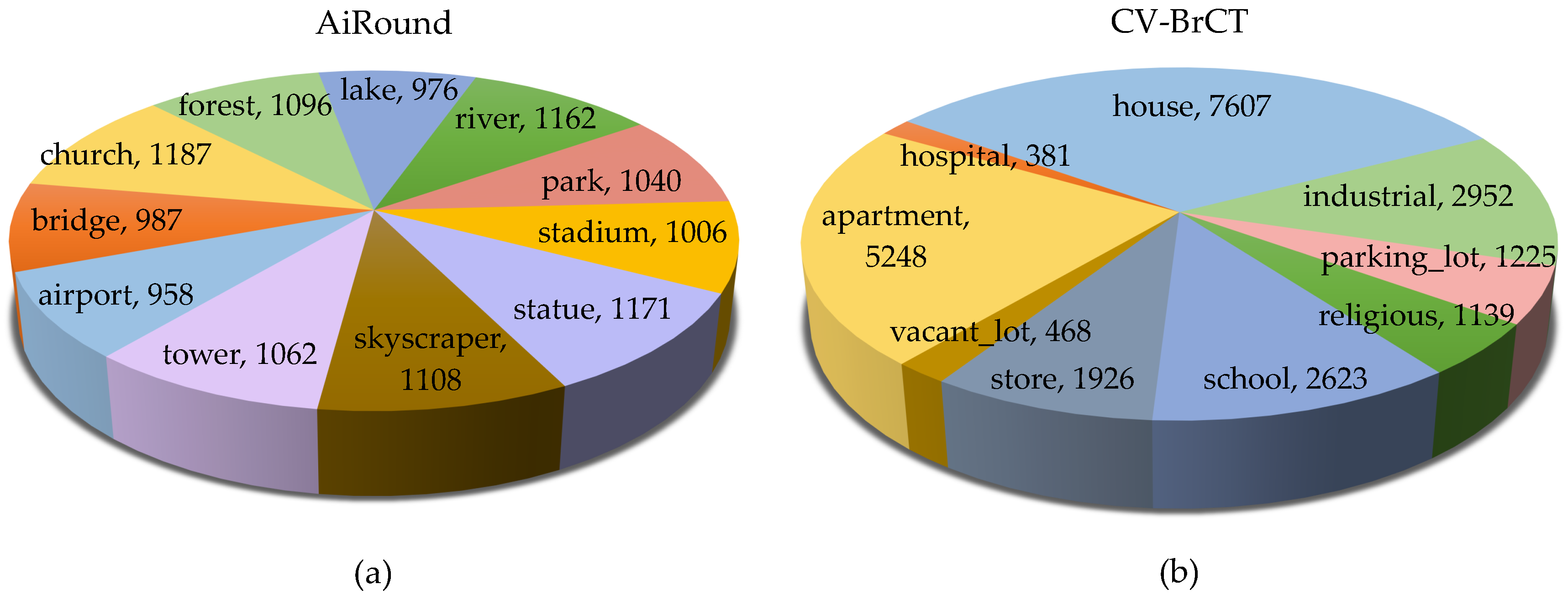
The AiRound dataset is a collection of landmarks from all over the world. It consists of images from three different views: the Sentinel-2 images, the high-resolution RGB aerial images, and the ground images. Sentinel-2 images have a size of 224 × 224 pixels. Aerial images have a size of 500 × 500 pixels. Ground images are obtained from two different ways, namley, Google Places’ database and Google Images. Thus they have different sizes. Their labels are obtained from the publicly available data of the OpenStreetMap. As shown in Figure 2a, there are 11 different land use classes in AiRound with a total of 11,753 groups of images. The aerial and ground images are used in our experiments.

The CV-BrCT dataset contains 23,569 pairs of images in 9 classes: apartment, hospital, house, industrial, parking lot, religious, school, store, and vacant lot. Each pairs are composed of an aerial view image and a ground view image, both of which are 500 × 500 RGB images. The class distribution is shown in Figure 2b.

2.2. Overview

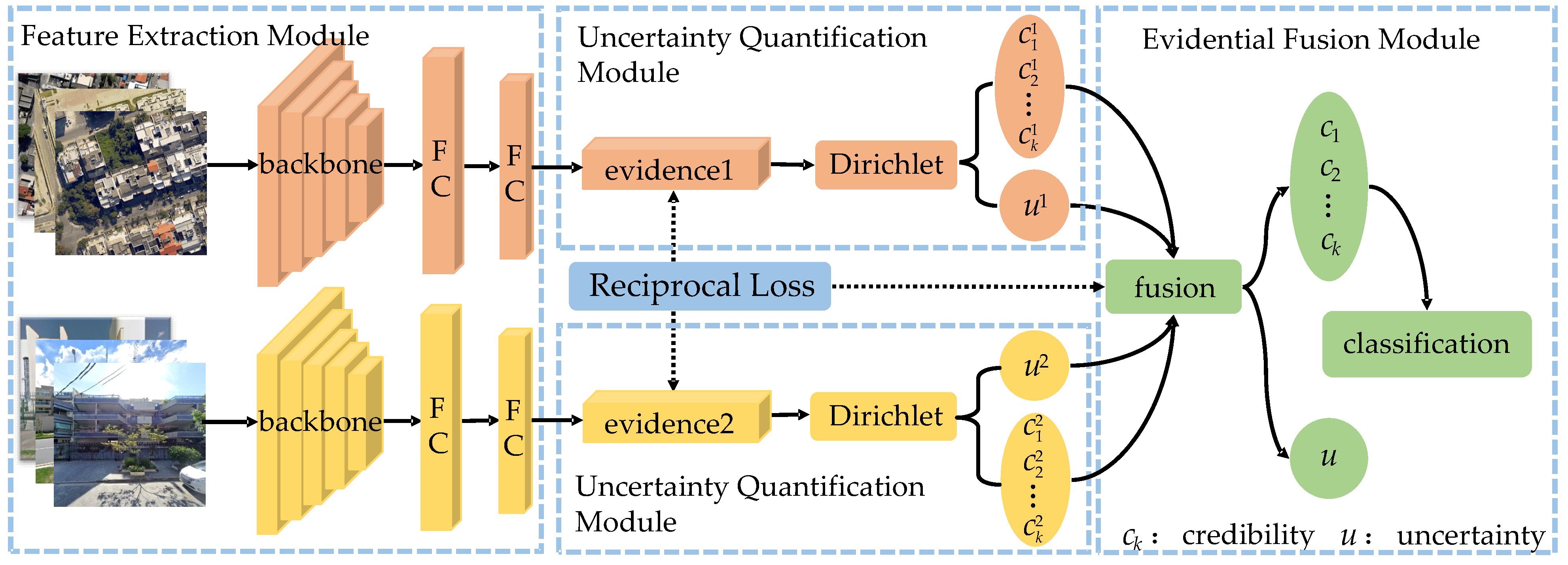
In the task of remote sensing scene classification on aerial-ground dual-view images, methods of data-level fusion and feature-level fusion are not satisfactory. This is because both the raw image and the visual feature of the aerial view differ too greatly from those of the ground view to meet the data requirements of data-level fusion and feature-level fusion: data-level fusion requires strict alignment of raw data from different views, well feature-level fusion requires that the dimensions and value ranges of intermediate features extracted from different views should not be too different. Recent works [18,31] show that decision-level fusion using a deep learning framework usually performs best. However, due to the lack of measurement of their credibility, multi-view decisions play equal roles during the fusion, despite the fact that their samples have unequal uncertainty. The proposed evidential fusion network (EFN) can assess the decision-making risk of each view by quantifying the sample uncertainty explicitly, and then assign different weight to the decisions base on their risks when fusing them. As a result, the final classification relies more on the view with lower decision-making risk therefore become more credible. The overall framework of EFN is shown in Figure 3. It can be further divided into three modules: the feature extraction module (FEM), the uncertainty quantification module (UQM) and the evidential fusion module (EFM).

The trained backbone extracts the features in each view and feeds them into a fully connected (FC) layer with a non-negative activation function to generate the “evidence vector” for uncertainty computation. Then, the evidence vector of each view is individually mapped to the concentration parameters of a Dirichlet distribution to estimate its credibility and uncertainty (see Section 2.3). Finally, they are fused by a weighted decision-level fusion (see Section 2.4).

The proposed FEM is divided into two subnets, each with a backbone and two extra FC layers. The backbones of two the subnets could be the same or different because the proposed approach is independent of them. It is this flexibility that makes the approach applicable to any network structure. Finally, the last softmax layer is replaced with a non-negative activation layer, such as softplus. This simple replacement operation makes the proposed approach extremely portable.

2.3. Uncertainty Estimation Based on Evidential Learning

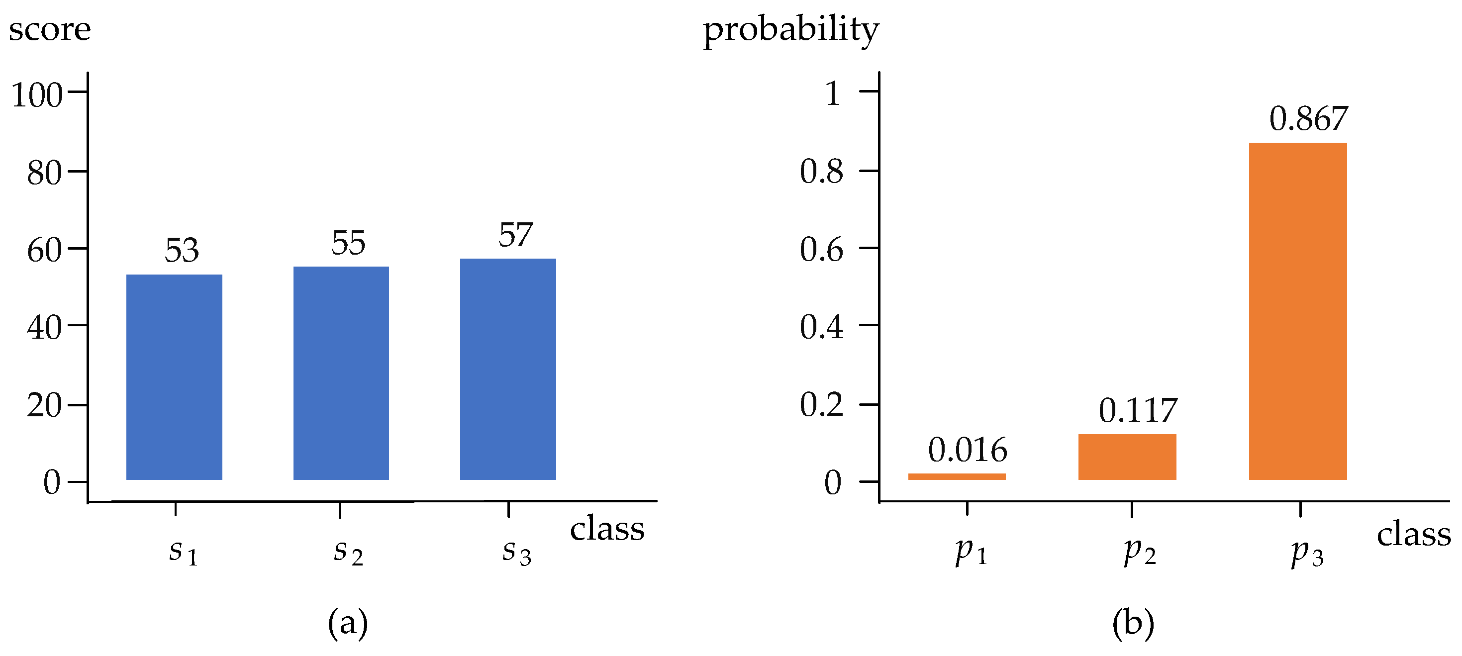
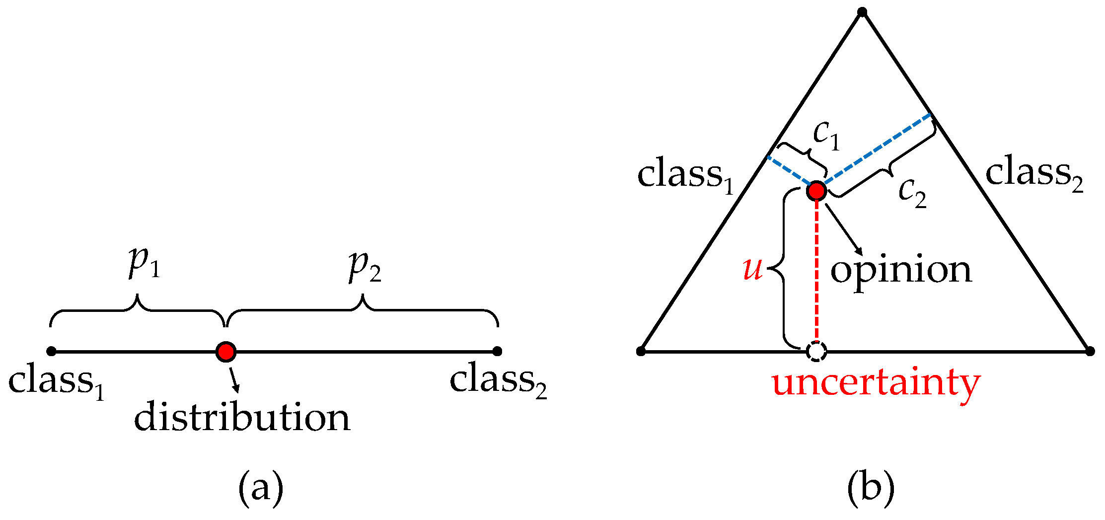
The use of the softmax operator to transform the output continuous activations into discrete class probabilities is widely recognized for classification networks. However, recent studies show that softmax operator has many shortcomings. Firstly, it may cause the issue of “over-confidence” [34]. For example, the scores of the three categories in Figure 4a are very close, indicating that the model is unsure about the input sample. However, after the softmax mapping in Figure 4b, the difference between the probabilities is greatly increased, giving the model the false impression of being very certain. Secondly, softmax can only provide a point estimate for the category probability of a sample without providing the associated uncertainty, which often leads to unreliable conclusions [35]. Figure 5 shows the difference between the softmax and an uncertainty estimation operation on a case of a binary classification problem. In Figure 5a, a class probability distribution is generated by softmax, where $p_i$ is the probability of class i, and we have $p_1+p_2=1$ and $p_1<p_2$, which means that the classifier is more inclined to classify the sample into class 2. However, we have no idea whether this prediction is credible.

To address the shortcomings of softmax, a non-negative activation function is used in place of the softmax operator to output the “evidence” for each class. Based on these evidences, the sample uncertainty can be described by the theory of evidence (TE) [36], which allows to explicitly express “ignorance” by taking the “base plane” (see Figure 6b) into consideration when building the “opinion space”. In Figure 5b, an “opinion” (the red point in the equilateral triangle) of sample is generated, where $c_i$ is the credibility of class i which is equal to the distance from the “opinion” to the side representing class i, and u is the sample uncertainty which is equal to the distance from the “opinion” to the base. It is well known that the sum of the distances from any point in an equilateral triangle to its three sides is equal to the height of the equilateral triangle. When setting the height of the equilateral triangle to 1, We have $c_1+c_2+u=1$ and $p_1<p_2<u$, which means that the classifier is more likely to find the sample unreliable than to make a binary decision. Figure 6 shows examples with three classes where the opinion equilateral triangle in Figure 5 rises its dimension to become a opinion tetrahedron [37]. In a more general sense, in a space with K classes, the K credibility values $c_k$ and the uncertainty u are both non-negative and sum to one, that is,

$$u+\sum _{k=1}^K{c}_k=1,$$

(1)

where $u\ge 0$ and $c_k\ge 0$ for $k=1,2,\cdots ,K$, denote the overall uncertainty and the credibility of k-th class respectively. For each view, the credibility of each class can be calculated using the evidence of each class. The non-negative evidence set of a sample can be denoted as $\mathbf{e}=[e_1,e_2,\cdots ,e_K]$. Let $e_k$ be the evidence of k-th class of the sample, the credibility $c_k$ and the uncertainty u can be calculated as

$$c_k=\frac{e_k}{{\sum }_{k=1}^K(e_k+1)},$$

(2)

$$u=\frac{K}{{\sum }_{k=1}^K(e_k+1)}.$$

(3)

The notion of TE could be further formalized as a Dirichlet distribution [37] with concentration parameter

$${\alpha }_k=e_k+1.$$

(4)

That is, the credibility and uncertainty can be easily obtained from the corresponding Dirichlet distribution using the following equations respectively:

$$c_k=\frac{{\alpha }_k-1}{{\alpha }_0},$$

(5)

$$u=\frac{K}{{\alpha }_0},$$

(6)

$${\alpha }_0=\sum _{k=1}^K{\alpha }_k.$$

(7)

For a K-classification problem, the concentration parameter $\mathbf{\alpha }=[{\alpha }_1,{\alpha }_2,\cdots ,{\alpha }_K]$, and the Dirichlet distribution is given by

$$D\left(\mathbf{p}\right|\mathbf{\alpha })=\left\{\begin{array}{cc}\frac{1}{B\left(\mathbf{\alpha }\right)}\prod _{k=1}^K{p}_k^{{\alpha }_k-1}\hfill & \mathbf{p}\in S_K\hfill \\ 0\hfill & otherwise\hfill \end{array}\right.,$$

(8)

where $B\left(\mathbf{\alpha }\right)$ is a K-dimensional multivariate beta function and ${\mathcal{S}}_K$ is the K-dimensional unit simplex,

$${\mathcal{S}}_K=\left\{\mathbf{p}\right|\sum _{k=1}^K{p}_k=1and0\le p_1,p_2,\cdots ,p_K\le 1\}.$$

(9)

Therefore, the concentration parameter of the Dirichlet distribution is thus associated with the evidence of each class. Up to now, the TEB-SUQ is ready to be used on both views of aerial and ground images to measure the decision-making risk during their fusion.

2.4. Evidential Fusion

As mentioned in Section 1, directly fusing the softmax outputs of the views will ignore their decision-making risks, resulting in unreliable results. In order to reduce the weight of the view with higher risk, a novel decision-level fusion strategy, namely Evidential Fusion is proposed based on Equations (2) and (3). Evidential fusion uses the sample uncertainty of each view as its decision-making risk to allocate the weight in the final prediction.

To be more precise, the opinions ${\mathcal{O}}^1=\{c_1^1,c_2^1,\dots ,c_K^1,u^1\}$ and ${\mathcal{O}}^2=\{c_1^2,c_2^2,\dots ,c_K^2,u^2\}$ of the two views are obtained after the UQM, where the superscripts denote the number of different views. The final decision opinions $\mathcal{O}=\{c_1,c_2,\dots ,c_K,u\}$ is then calculated as follows:

$$c_k=\frac{1}{\lambda }[c_k^1{c}_k^2+(1-u^1)c_k^1+(1-u^2)c_k^2],$$

(10)

$$u=\frac{1}{\lambda }{u}^1{u}^2,$$

(11)

$$\lambda =u^1{u}^2+{(1-u^1)}^2+{(1-u^2)}^2+\sum _{k=1}^K{c}_k^1{c}_k^2,$$

(12)

where $\lambda$ is scale factor to perform the normalization and to ensures that Equation (1) still holds after fusion.

After obtaining the final decision opinion $\mathcal{O}$ from the fusion of two views, the fused evidence $e_k$ of the k-th class can be calculated according to the following equation:

$$e_k=\frac{K·c_k}{u},$$

(13)

and the concentration parameters ${\alpha }_k$ of the Dirichlet distribution of the k-th class can be updated by Equation (4) to calculate the loss during training step and the category with the largest $e_k$ is the final predicted label during test step.

An example is given to demonstrate how the the proposed evidential fusion works in Figure 7. A multiplication fusion on the softmax outputs of aerial-ground dual-view images is shown in Figure 7a and the proposed evidential fusion on the UQM outputting opinions is shown in Figure 7b, which obtains a more credible classification result based on the sample uncertainty.

2.5. Reciprocal Loss

To train the proposed EFN in Figure 3, the following loss function is designed and then adopted on each view:

$$L\left(\mathbf{\alpha }\right)=\sum _{i=1}^N(L_{pc}\left({\mathbf{\alpha }}_i\right)+L_{nc}\left({\mathbf{\alpha }}_i\right)),$$

(14)

$$L_{pc}\left({\mathbf{\alpha }}_i\right)=\sum _{k=1}^K{y}_{ik}\left[\psi \left({\alpha }_{i0}\right)-\psi \left({\alpha }_{ik}\right)\right],$$

(15)

$$L_{nc}\left({\mathbf{\alpha }}_i\right)=\sum _{k=1}^K(1-y_{ik})\frac{1}{\psi \left({\alpha }_{i0}\right)-\psi \left({\alpha }_{ik}\right)},$$

(16)

where $L_{pc}\left({\mathbf{\alpha }}_i\right)$ and $L_{nc}\left({\mathbf{\alpha }}_i\right)$ are positive-class loss and negative-class loss of the i-th sample respectively, $\psi (·)$ is the digamma function which is monotonically increasing in $(0,+\infty )$, ${\alpha }_{i0}$ is consistent with Equation (7), K is the number of classes and N is the number of samples.

As shown in Equation (14), the proposed loss function clearly separates the penalty terms of the positive and negative classes, making it easy to interpret. Furthermore, Equations (15) and (16) show that the positive-class loss and the negative-class loss are reciprocal. More specifically, since ${\alpha }_{ik}=e_{ik}+1$ and $e_{ik}>0$, so $\psi \left({\alpha }_{ik}\right)$ is monotonically increasing with ${\alpha }_{ik}$, while $L_{pc}\left({\mathbf{\alpha }}_i\right)$ is monotonically decreasing with ${\alpha }_{ik}$, which ensures that the positive class of each sample generates more evidence. On the contrary, $L_{nc}\left({\mathbf{\alpha }}_i\right)$ is monotonically increasing with ${\alpha }_{ik}$ to ensure that negative classes of each sample generate less evidence. Next, taking $L_{pc}\left({\mathbf{\alpha }}_i\right)$ as an example, how the proposed Reciprocal Loss is related to the Dirichlet distribution will be derived.

For multi-class classification tasks, the cross-entropy loss function (CE Loss) is most commonly used. For a particular sample, its CE Loss can be calculated by

$$L_{ce}=-\sum _{k=1}^K{y}_{k}log{p}_k,$$

(17)

where $p_k$ is the predicted probability of the k-th class, $y_k$ is its class label and $y_k=1$ for positive classes and $y_k=0$ for negative classes. In the proposed EFN, the evidence vector of a sample $e$ obtained from the FEM can be mapped to the concentration parameters $\mathbf{\alpha }$ of the Dirichlet distribution $D\left(\mathbf{p}\right|\mathbf{\alpha })$ by using Equation (4). Thus the Bayes risk of cross-entropy loss $L_{cer}\left(\mathbf{\alpha }\right)$ can be calculated as

$$\begin{array}{cc}\hfill L_{cer}\left(\mathbf{\alpha }\right)& =\int L_{ce}D\left(\mathbf{p}\right|\mathbf{\alpha })d\mathbf{p}\hfill \\ \hfill & =\int (-\sum _{k=1}^K{y}_{k}log{p}_k)D\left(\mathbf{p}\right|\mathbf{\alpha })d\mathbf{p}.\hfill \end{array}$$

(18)

Since $p_k$ is a $D\left(\mathbf{p}\right|\mathbf{\alpha })$ random variable, the functions $log{p}_k$ are the sufficient statistics of the Dirichlet distribution. Thus, the exponential family differential identities can be used to get an analytic expression for the expectation of $log{p}_k$ [38]:

$$\begin{array}{cc}\hfill {\mathbb{E}}_{D\left(\mathbf{p}\right|\mathbf{\alpha })}(log{p}_k)& =\int (log{p}_k)D\left(\mathbf{p}\right|\mathbf{\alpha })d\mathbf{p}\hfill \\ \hfill & =\psi \left({\alpha }_k\right)-\psi \left({\alpha }_0\right).\hfill \end{array}$$

(19)

In this regard, Equation (18) can be expanded further as

$$\begin{array}{cc}\hfill L_{cer}\left(\mathbf{\alpha }\right)& =\int (-\sum _{k=1}^K{y}_{k}log{p}_k)D\left(\mathbf{p}\right|\mathbf{\alpha })d\mathbf{p}\hfill \\ \hfill & =-\sum _{k=1}^K{y}_k\int (log{p}_k)D\left(\mathbf{p}\right|\mathbf{\alpha })d\mathbf{p}\hfill \\ \hfill & =-\sum _{k=1}^K{y}_k\left[\psi \left({\alpha }_k\right)-\psi \left({\alpha }_0\right)\right]\hfill \\ \hfill & =\sum _{k=1}^K{y}_k\left[\psi \left({\alpha }_0\right)-\psi \left({\alpha }_k\right)\right].\hfill \end{array}$$

(20)

Given that the Equation (20) can only penalize the positive class, $L_{cer}$ can be written as $L_{pc}$. We finally have $L_{pc}\left({\mathbf{\alpha }}_i\right)$ in Equation (15) for the case of all samples.

In order to ensure that both views can provide reasonable opinions for scene classification and thus improve the overall opinion after fusion, the final multi-view global Reciprocal Loss is used:

$$L_{global}=L^1+L^2+L_{fused},$$

(21)

where $L^1$, $L^2$ are the Reciprocal Loss (Equation (14)) for the first view and second view, respectively, and $L_{fused}$ is obtained using Equation (14) on the fused parameters by Equations (4), (10), (11) and (13).

3. Results

3.1. Experimental Setup

For both datasets of AiRound and CV-BrCT, we randomly selected 80% of the samples from each class as the training/validation set and the remaining 20% as the test set to form one data split. All the test results except for Section 3.2.1 are the mean results of 10 splits. The training/validation set was randomly divided into the training set and validation set according to the ratio of 9:1.

All models were simulated by PyTorch on a computer with a GTX 1080Ti graphics card. The details during training are as follows. Batch size: 128; the number of epochs: 200 for feature extraction and credible fusion, respectively, and all the best models on validation data are saved, learning rate schedules: Cosine decay with the initial value of 0.01, optimizer: SGD for feature extraction and Adam for credible fusion, weight decay: 0.1, and momentum of SGD: 0.9. All models of feature extraction are trained by fine-tuning the officially published pre-trained ones.

To quantitatively evaluate the performance of each model, we used the classification accuracy (Acc) and F1-score (F1) as metrics. Acc is calculated by the ratio of the number of correctly predicted test samples to the total number of test samples. F1 is calculated by the ratio of twice the product of precision and recall to the sum of them.

3.2. Ablation Study

3.2.1. Validation for the Effectiveness of Uncertainty Estimation

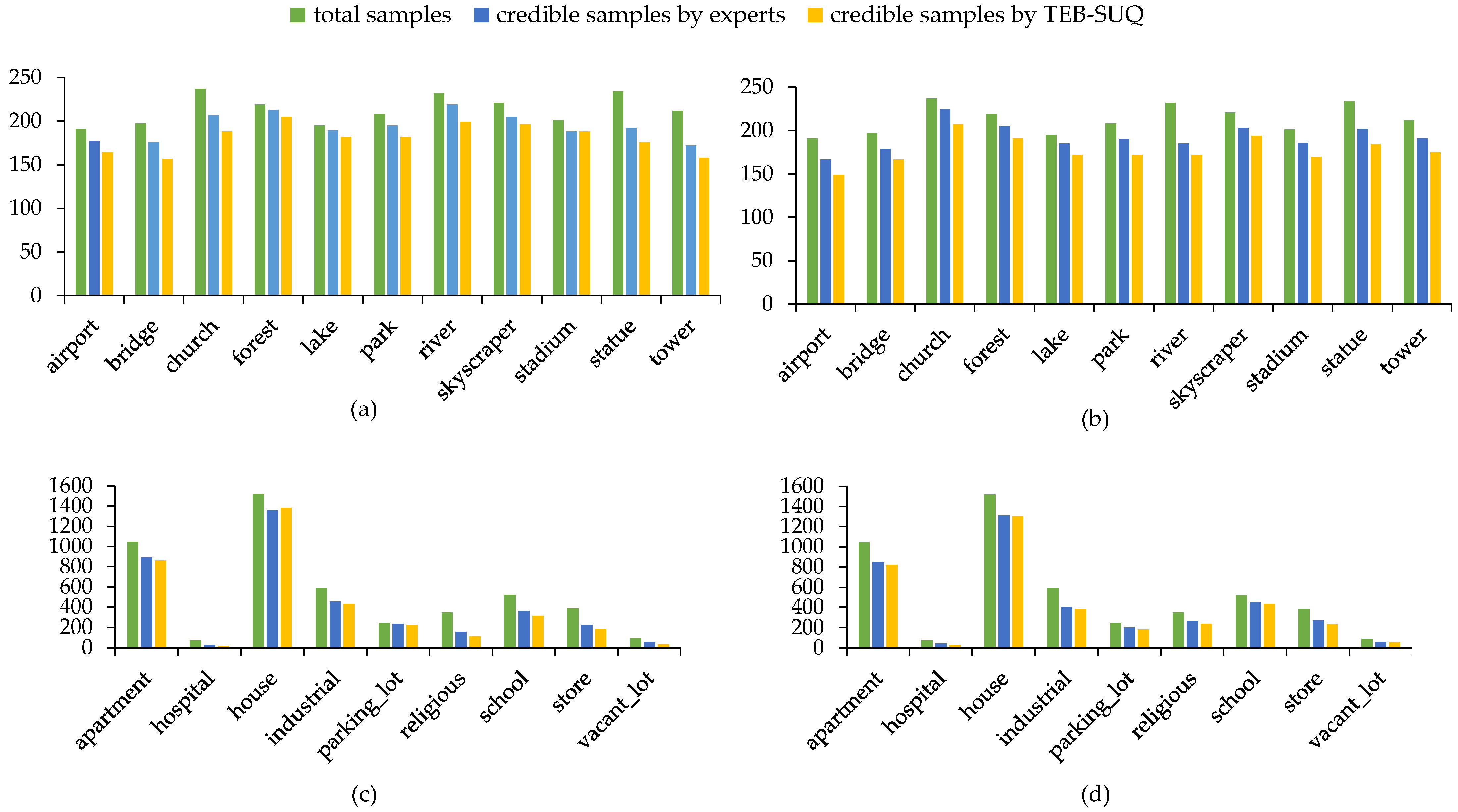
In order to validate the effectiveness of the TEB-SUQ in measuring sample uncertainty, a subjective evaluation of sample credibility was performed. All test samples from the two datasets (2347 pairs of AiRound and 4830 pairs of CV-BrCT) were evaluated by nine urban planning experts from the Qingdao Research Institute of Urban and Rural Construction based on whether their image content matched the label. A vote of nine experts determines the final conclusion (credible or uncertain) of each test sample. For the TEB-SUQ, an appropriate threshold $u_{th}$ was set to distinguish between credible and uncertain samples. The number of credible samples calculated using $u\le 0.4$ ($n_k$ for the k-th class) was compared to the one generated by experts’ votes ($m_k$ for the k-th class) in each class of each view of the two datasets in Figure 8.

Table 1. The average error of the TEB-SUQ relative to subjective evaluation.

Views *	A-AiRound	G-AiRound	A-CV-BrCT	G-CV-BrCT
$\overline{\sigma }$	0.065	0.078	0.183	0.090

* A- for the aerial view and G- for the ground view.

shows the average error $\overline{\sigma }$ of the TEB-SUQ relative to subjective evaluation of each view using

$$\overline{\sigma }=\frac{1}{K}\sum _{k=1}^K\frac{|n_k-m_k|}{m_k},$$

(22)

where K is the total number of classes.

As can be observed from Table 1, except for the aerial view of CV-BrCT, the relative error between the predicted number of credible samples and the subjective evaluation in other views is less than 0.1, proving that the proposed sample uncertainty estimation approach is effective.

3.2.2. Validation for the Effectiveness of the Reciprocal Loss

The widely used loss function for evidential deep learning (EDL Loss for short) consists of a term of general classification loss and a term of Kullback–Leibler (KL) divergence of two Dirichlet distributions with an extra annealing coefficient [33]. It is formally too complex and difficult to train, in contrast to the proposed Reciprocal Loss (Equation (14) to Equation (16)). Scene classification performances of EDL Loss and the proposed Reciprocal Loss are shown in

Table 2. Performances (%) ± STD of different loss functions.

Loss Functions	AiRound		CV-BrCT
	Acc	F1	Acc	F1
EDL-CE Loss [33]	90.23 ± 0.32	90.64 ± 0.29	86.98 ± 0.17	81.56 ± 0.34
EDL-MSE Loss [33]	90.44 ± 0.03	91.02 ± 0.02	86.24 ± 0.02	80.89 ± 0.01
Reciprocal Loss	92.16 ± 0.31	92.49 ± 0.25	88.21 ± 0.26	83.57 ± 0.29

, where in EDL-CE Loss, the first term of general classification loss is CE-like (see Equation (4) in the Ref. [33]), whereas in EDL-MSE Loss, it is MSE-like (see Equation (5) in the Ref. [33]). All results were obtained using VGG-11 [39] as the backbone with the same training setting and fusion strategy. The annealing coefficient in EDL was calculated as $min(1.0,t/10)\in [0,1]$, where t is the index of the current training epoch. It is clear that the use of Reciprocal Loss resulted in improved performances.

3.2.3. Validation for the Effectiveness of the Evidential Fusion Strategy

As described in Section 2.2, the proposed approach is backbone-independent, allowing it to be flexibly matched with different deep feature extraction networks. In this experiment, three of the most common backbones are used to compare the performance on scene classification task before and after using different fusion strategies. In the columns of single views in

Table 3. Classification accuracy (%) ± STD of single views and after decision-level fusion on AiRound.

Views		AlexNet [40]	VGG-11 [39]	ResNet-18 [41]
Single Views	Aerial-s	76.96 $\pm 0.52$	82.75 $\pm 0.61$	80.93 $\pm 0.49$
(softmax)	Ground-s	71.35 $\pm 0.24$	77.10 $\pm 0.28$	76.68 $\pm 0.19$
Single Views	Aerial-e	76.04 $\pm 0.46$	82.64 $\pm 0.49$	80.83 $\pm 0.52$
(evidential)	Ground-e	70.96 $\pm 0.25$	76.99 $\pm 0.17$	76.36 $\pm 0.22$
Decision-	Sum [31]	84.02 $\pm 0.47$	87.75 $\pm 0.38$	88.02 $\pm 0.25$
Level Fusion	Product [31]	86.74 $\pm 0.25$	90.41 $\pm 0.27$	89.56 $\pm 0.24$
Strategies	Proposed	88.12 ± 0.23	92.16 ± 0.31	91.02 ± 0.35

and

Table 4. Classification accuracy (%) $\pm \mathrm{STD}$ of single views and after decision-level fusion on CV-BrCT.

Views		AlexNet [40]	VGG-11 [39]	ResNet-18 [41]
Single Views	Aerial-s	84.63 $\pm 0.24$	87.11 $\pm 0.42$	86.74 $\pm 0.38$
(softmax)	Ground-s	68.01 $\pm 0.12$	71.43 $\pm 0.22$	70.96 $\pm 0.25$
Single Views	Aerial-e	84.37 $\pm 0.10$	87.06 $\pm 0.38$	86.18 $\pm 0.29$
(evidential)	Ground-e	66.36 $\pm 0.25$	70.15 $\pm 0.29$	70.86 $\pm 0.24$
Decision-	Sum [31]	85.26 $\pm 0.45$	86.70 $\pm 0.58$	85.59 $\pm 0.62$
Level Fusion	Product [31]	86.52 $\pm 0.25$	87.21 $\pm 0.22$	86.83 $\pm 0.18$
Strategies	Proposed	88.02 ± 0.28	88.21 ± 0.26	87.95 ± 0.19

, the ”-s” represents the traditional deep learning (that is, softmax deep learning) approach where the softmax layer and CE Loss are used during the training phase, and the class corresponding to the maximum probability calculated by the softmax operator is used as the prediction result during the test phase. Additionally, ”-e” denotes the evidential deep learning approach proposed in Section 2.3 and Section 2.5 where the softmax layer is replaced by the softplus layer and the proposed Reciprocal Loss are used for training. The class corresponding to the maximum evidence value is used as the prediction result during the test. In the columns of fusion strategies, two common decision level fusion strategies (sum and product) [31] are used as baseline approaches to compare the proposed evidential fusion. The best results are highlighted in bold.

The following observations can be made from Table 3 and Table 4. First, all of the fusion results are superior to any single view result. This demonstrates that information from multi-views can significantly improve classification accuracy. Second, the performance of the two single views obtained through evidential deep learning is marginally worse than that of the corresponding single view obtained through softmax deep learning. This is due to the fact that when the uncertainty of some samples is high, evidential deep learning focuses more on estimating the uncertainty values as accurately as possible, which may result in a loss of classification accuracy for these samples. However, in terms of sample quality, the category labels of these high-uncertainty samples lack actual semantics. It also does not matter whether their predictions are correct or incorrect. It makes more sense to quantify their uncertainty. Last but not least, the evidential fusion strategy proposed in this paper outperforms the other two baseline fusion approaches, which demonstrates the efficacy of evidential fusion in the task of multi-view remote sensing scene classification.

3.3. Comparison Experiment with Different Fusion Approaches at Data-Level, Feature-Level and Decision-Level

In Section 3.2, the effectiveness of three innovative contributions in this paper (namely TEB-SUQ, Evidential Fusion, and Reciprocal Loss) was validated, respectively. In this section, more multi-view fusion methods are compared with the proposed approach to assess its overall performance on the task of aerial-ground dual-view remote sensing scene classification. As mentioned in Section 1, existing multi-view fusion methods can be roughly classified as data-level, feature-level, and decision-level. In this experiment, one data-level fusion method (six-channel [42]), two feature-level fusion methods (feature concatenation [31] and CILM [43]), and five decision-level fusion methods (maximum [31], minimum [31], sum [31], product [31] and SFWS [44]) were chosen to compare with the proposed evidential fusion. These methods are briefly described below.

• Six-channel [42]: This method concatenates the RGB channels of the paired aerial view and ground view images into a six-channel image as the input of a CNN.
• Feature concatenation [31]: A Siamese-like CNN is used to concatenate the intermediate feature tensors before the first convolution layer that doubles its amount of kernels.
• CILM [43]: The loss function of contrast learning is combined with CE Loss in this method, allowing the features extracted by the two subnetworks to be fused without sharing any weight.
• Maximum [31]: Each view employs an independent DNN to obtain its prediction result, which consists of a class label and its probability. The final prediction is the class label corresponding to the maximum of the class probabilities predicted by each view.
• Minimum [31]: Each view employs an independent DNN to obtain its prediction result, which consists of a class label and its probability. The final prediction is the class label corresponding to the minimum of the class probabilities predicted by each view.
• Sum [31]: Each view employs an independent DNN to generate a vector containing probabilities for each class. The fused vector is the sum of single view vectors. The final prediction result is the class label corresponding to the largest element in the fused vector.
• Product [31]: Each view employs an independent DNN to generate a vector containing probabilities for each class. An elementwise multiplication is performed between single view vectors to obtain the fused vector. The final prediction result is the class label corresponding to the largest element in the fused vector.
• SFWS (Softmax Feature Weighted Strategy) [44]: Each view employs an independent DNN to obtain a vector containing probabilities for each class. Then, the matrix nuclear norm of the vector is computed as the weight of the fusion. The final prediction result is the class label corresponding to the largest element in the fused vector.

Table 5. Classification accuracy (%) $\pm \mathrm{STD}$ using different fusion methods on AiRound.

Methods	AlexNet [40]	VGG-11 [39]	Inception [45]	ResNet-18 [41]	DenseNet [46]
Six-Ch. [42]	70.19 $\pm 0.23$	72.34 $\pm 0.21$	71.76 $\pm 0.24$	71.29 $\pm 0.26$	71.57 $\pm 0.25$
Concat. [31]	82.52 $\pm 0.32$	84.69 $\pm 0.41$	83.91 $\pm 0.45$	83.56 $\pm 0.39$	83.72 $\pm 0.42$
CILM [43]	83.49 $\pm 0.17$	85.72 $\pm 0.19$	85.05 $\pm 0.15$	84.72 $\pm 0.21$	84.91 $\pm 0.20$
Max. [31]	84.86 $\pm 0.36$	88.17 $\pm 0.34$	88.39 $\pm 0.33$	88.21 $\pm 0.38$	89.96 $\pm 0.35$
Min. [31]	85.52 $\pm 0.23$	89.56 $\pm 0.25$	89.12 $\pm 0.27$	88.42 $\pm 0.22$	90.41 $\pm 0.27$
Sum [31]	84.02 $\pm 0.47$	87.75 $\pm 0.38$	88.05 $\pm 0.30$	88.02 $\pm 0.25$	89.88 $\pm 0.31$
Product [31]	86.74 $\pm 0.25$	90.41 $\pm 0.24$	90.02 $\pm 0.14$	89.56 $\pm 0.24$	91.16 $\pm 0.17$
SFWS [44]	85.94 $\pm 0.17$	89.61 $\pm 0.34$	89.18 $\pm 0.12$	88.95 $\pm 0.26$	90.05 $\pm 0.37$
Proposed	88.12 ± 0.23	92.16 ± 0.31	91.41 ± 0.18	91.02 ± 0.35	92.16 ± 0.19

and

Table 6. Classification accuracy (%) $\pm \mathrm{STD}$ using different fusion methods on CV-BrCT.

Methods	AlexNet [40]	VGG-11 [39]	Inception [45]	ResNet-18 [41]	DenseNet [46]
Six-Ch. [42]	71.92 $\pm 0.26$	73.46 $\pm 0.24$	75.26 $\pm 0.25$	73.25 $\pm 0.28$	74.19 $\pm 0.27$
Concat. [31]	81.86 $\pm 0.42$	83.25 $\pm 0.39$	84.65 $\pm 0.38$	83.28 $\pm 0.41$	84.24 $\pm 0.40$
CILM [43]	83.10 $\pm 0.20$	84.32 $\pm 0.19$	85.22 $\pm 0.16$	84.31 $\pm 0.17$	85.19 $\pm 0.22$
Max. [31]	85.52 $\pm 0.24$	86.74 $\pm 0.39$	86.70 $\pm 0.41$	85.84 $\pm 0.43$	86.95 $\pm 0.38$
Min. [31]	86.02 $\pm 0.21$	86.95 $\pm 0.27$	86.95 $\pm 0.28$	86.24 $\pm 0.35$	87.02 $\pm 0.25$
Sum [31]	85.26 $\pm 0.45$	86.70 $\pm 0.58$	86.24 $\pm 0.35$	85.59 $\pm 0.62$	86.85 $\pm 0.39$
Product [31]	86.52 $\pm 0.25$	87.21 $\pm 0.22$	87.02 $\pm 0.21$	86.83 $\pm 0.18$	87.54 $\pm 0.17$
SFWS [44]	86.21 $\pm 0.14$	86.95 $\pm 0.22$	86.73 $\pm 0.21$	86.52 $\pm 0.16$	87.21 $\pm 0.25$
Proposed	88.02 ± 0.28	88.21 ± 0.26	88.21 ± 0.23	87.95 ± 0.19	88.34 ± 0.20

show the performance of the fusion methods discussed above on AiRound and CV-BrCT, respectively, when different backbones are used. The following observations can be made. First, methods of the data-level fusion class performed the worst, while methods of the decision-level fusion class won across the board. This observation is consistent with the discussion of data-level fusion and feature-level fusion in Section 2.2. The performance of the fusion improves as the features involved in it become more abstract. This also explains why CILM outperforms feature concatenation among the two feature-level fusion methods: CILM lacks a shared weight structure, making it more similar to decision-level fusion in form. Second, among the decision-level fusion methods, sum and maximum perform nearly identically, and both perform slightly worse than minimum. This result may seem counter-intuitive at first. In fact, it confirms the overconfidence issue caused by the softmax mentioned in Section 2.3 (see Figure 4 and Figure 5): an overestimated prediction is more likely to be incorrect. Last but not least, product and the proposed evidential fusion stand out among all the fusion methods, and the latter outperforms the former. In fact, Equation (10) can be seen as an enhancement of the product method. The inclusion of sample uncertainty breaks down the equality of views in the fusion: views with lower u values are given more weight adaptively.

Table 7. Training time (ms per sample) $\pm \mathrm{STD}$ using different fusion methods.

Datasets	Training Time
	Six-Ch. [42]	Concat. [31]	CILM [43]	Dec.-Lev. [31,44]	Proposed
AiRound	9.16 ± 0.01	9.21 $\pm 0.02$	9.38 $\pm 0.02$	9.37 $\pm 0.01$	9.42 $\pm 0.01$
Cv-BrCT	8.01 ± 0.01	8.06 $\pm 0.02$	8.20 $\pm 0.02$	8.19 $\pm 0.01$	8.23 $\pm 0.01$

shows the training time of the fusion methods discussed above using VGG-11 as the backbone. The proposed evidential fusion approach takes $2.72\%$ more time than the most time-efficient model (Six-Ch.) and only $0.51\%$ more time than other decision-level fusion approaches (Dec.-Lev.). During inference, the added time of the proposed method is negligible and therefore does not affect the actual use.

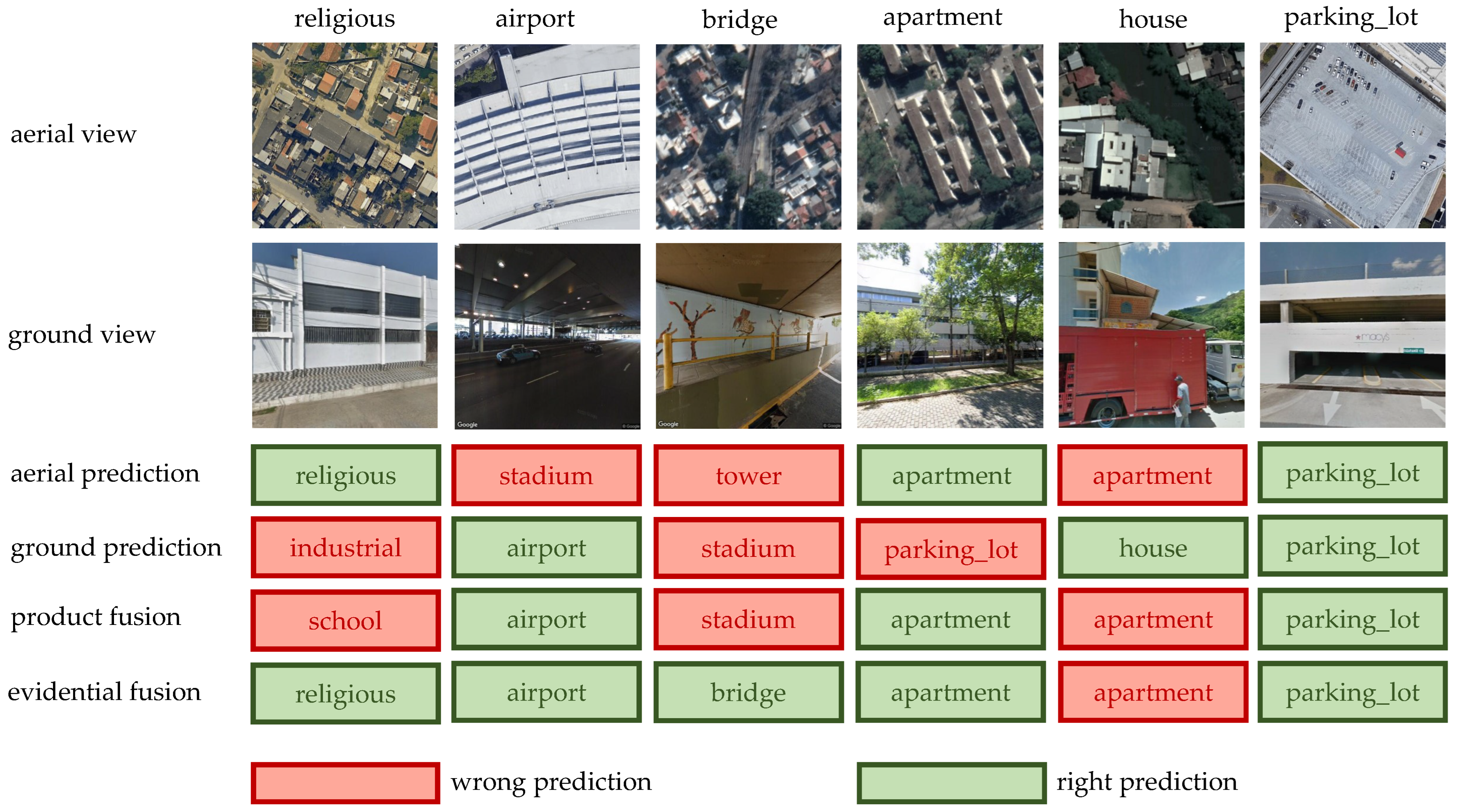
Finally, on all backbones of both datasets, the proposed evidential fusion approach outperforms the best decision-level fusion method by $1.26\%$, the best feature-level fusion method by $4.96\%$ and the data-level fusion method by $17.04\%$. Examples of predictions are shown in Figure 9.

4. Discussion

4.1. Discussion on Uncertainty Estimation

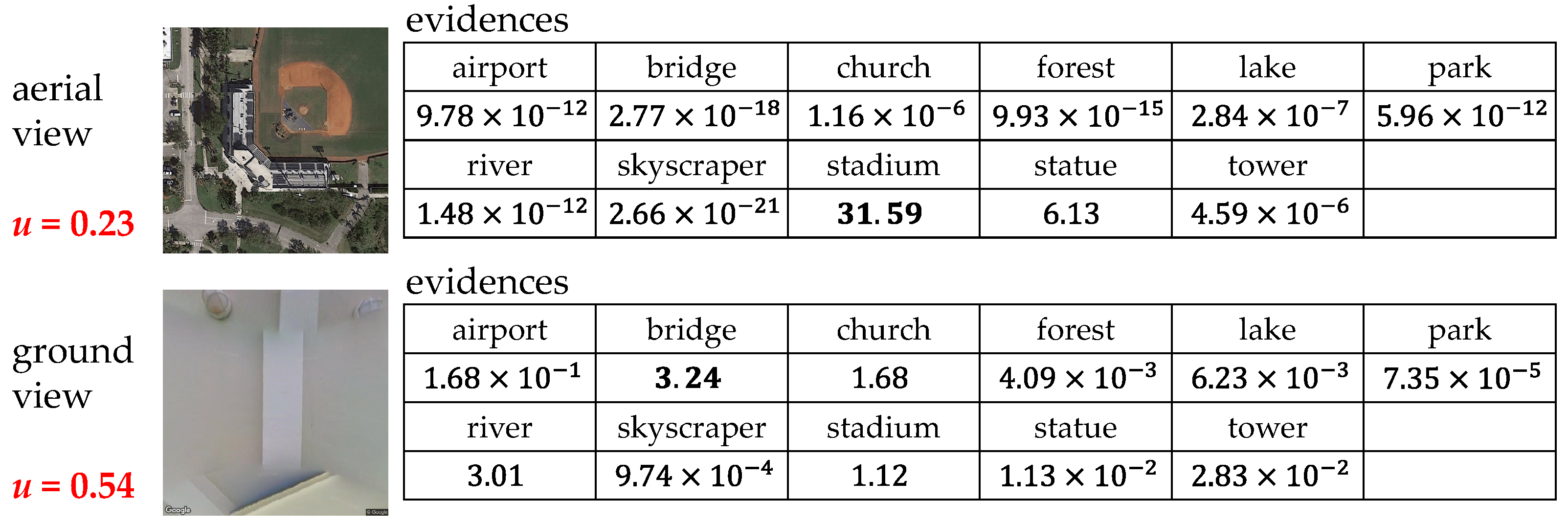
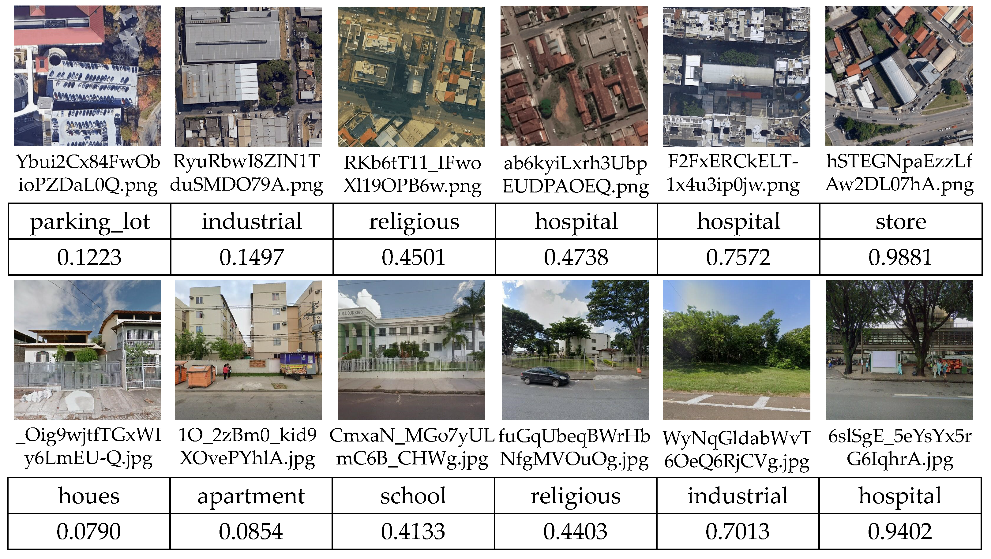
Figure 10 shows one case study of the class “stadium” in AiRound. By the TEB-SUQ, the uncertainties and evidence of two images in different views were obtained. The evidence values bigger than 1.00 of the aerial image are 31.59 (stadium) and 6.13 (statue), showing a good concentration. Accordingly, its uncertainty is only about 0.23. However, the evidence values bigger than 1.00 of the ground image are 3.24 (bridge), 3.01 (river), 1.68 (church) and 1.12 (stadium), whose distribution is more dispersed. Accordingly, its uncertainty is about 0.54, suggesting that the model is less than half as confident about its predictions. As can be seen from the images, the above conclusions are intuitive. More cases of the uncertainty of samples in the CV-BrCT datasets are shown in Figure 11, whose classes are random selected.

More statistically, Figure 12 shows the uncertainty distributions of each view samples in the test sets of the AiRound and CV-BrCT. The figures clearly show that the samples of AiRound are distributed more densely in parts with lower uncertainty and have higher peak values. This advantage is even more visible in the ground view (Figure 12b). In other words, after the calculation by the TEB-SUQ, the quality of AiRound is higher than that of CV-BrCT, especially in the ground view. This conclusion is supported by the following facts. Firstly, CV-BrCT has more than twice the number of samples as AiRound. Secondly, unlike the average distribution of AiRound, the class distribution of CV-BrCT is a typical long-tail distribution (Figure 2b). It is well-understood that increasing the number of samples and unbalanced category distribution will result in a decrease in data quality. Last but not least, the methodologies used to collect the ground view images for the two datasets differ [31]. The ground view images of AiRound are largely derived from the Google Places’ database, which is a well-known high-quality dataset. The ground view images of CV-BrCT, on the other hand, were all obtained by the Google Images search engine, meaning that image quality cannot be guaranteed.

4.2. Discussion on Loss Functions

Figure 13 shows the training and validation loss using EDL Loss and Reciprocal Loss (Equation (21)) with the same setting. Significant overfitting occurred during training using EDL Loss. It has been significantly improved since switching to Reciprocal Loss.

5. Conclusions

Deep learning models are easily influenced by data quality, especially when dealing with massive amounts of data [47,48]. Li’s team proposed the concept of “trustworthy AI” [49], with a focus on data quality. As multi-view data is increasingly used in various remote sensing tasks, the issue of data quality in the original single view becomes more apparent. In this paper, the theory of evidence was introduced to quantify the credibility of samples. On this basis, a decision-level multi-view fusion strategy was proposed to assign higher weights to views with lower decision-making risk. The proposed evidential fusion network achieves the best performance on the two classical datasets in the task of remote sensing scene classification on aerial-ground dual-view images, outperforms the best decision-level fusion method by $1.26\%$, the best feature-level fusion method by $4.96\%$ and the data-level fusion method by $17.04\%$.

Focusing on data quality in multi-view tasks is a new area of research, and much work remains to be done. First, there are few publicly available multi-view datasets for remote sensing tasks. Large-scale, instance-level aligned remote sensing multi-view data sets are urgently needed for public release for related research. Furthermore, effective objective evaluation of sample uncertainty estimation is lacking. Datasets with sample quality annotation have yet to appear in the field of remote sensing. Finally, more explicit representation methods of sample uncertainty need to be further explored.

References

1. Cheng, G.; Han, J.; Lu, X. Remote Sensing Image Scene Classification: Benchmark and State of the Art. Proc. IEEE 2017, 105, 1865–1883. [Google Scholar] [CrossRef] [Green Version]
2. Cheng, G.; Xie, X.; Han, J.; Guo, L.; Xia, G.S. Remote Sensing Image Scene Classification Meets Deep Learning: Challenges, Methods, Benchmarks, and Opportunities. IEEE J. Sel. Top. Appl. Earth Obs. Remote Sens. 2020, 13, 3735–3756. [Google Scholar] [CrossRef]
3. Zhou, Y.; Chen, P.; Liu, N.; Yin, Q.; Zhang, F. Graph-Embedding Balanced Transfer Subspace Learning for Hyperspectral Cross-Scene Classification. IEEE J. Sel. Top. Appl. Earth Obs. Remote Sens. 2022, 15, 2944–2955. [Google Scholar] [CrossRef]
4. Chen, L.; Cui, X.; Li, Z.; Yuan, Z.; Xing, J.; Xing, X.; Jia, Z. A New Deep Learning Algorithm for SAR Scene Classification Based on Spatial Statistical Modeling and Features Re-Calibration. Sensors 2019, 19, 2479. [Google Scholar] [CrossRef] [Green Version]
5. Wang, Q.; Liu, S.; Chanussot, J.; Li, X. Scene Classification With Recurrent Attention of VHR Remote Sensing Images. IEEE Trans. Geosci. Remote Sens. 2019, 57, 1155–1167. [Google Scholar] [CrossRef]
6. Li, B.; Guo, Y.; Yang, J.; Wang, L.; Wang, Y.; An, W. Gated Recurrent Multiattention Network for VHR Remote Sensing Image Classification. IEEE Trans. Geosci. Remote Sens. 2022, 60, 1–13. [Google Scholar] [CrossRef]
7. Qiao, Z.; Yuan, X. Urban land-use analysis using proximate sensing imagery: A survey. Int. J. Geogr. Inf. Sci. 2021, 35, 2129–2148. [Google Scholar] [CrossRef]
8. Baltrušaitis, T.; Ahuja, C.; Morency, L.P. Multimodal Machine Learning: A Survey and Taxonomy. IEEE Trans. Pattern Anal. Mach. Intell. 2019, 41, 423–443. [Google Scholar] [CrossRef] [Green Version]
9. Nunez, J.; Otazu, X.; Fors, O.; Prades, A.; Pala, V.; Arbiol, R. Multiresolution-based image fusion with additive wavelet decomposition. IEEE Trans. Geosci. Remote Sens. 1999, 37, 1204–1211. [Google Scholar] [CrossRef] [Green Version]
10. Amolins, K.; Zhang, Y.; Dare, P. Wavelet based image fusion techniques—An introduction, review and comparison. ISPRS J. Photogramm. Remote Sens. 2007, 62, 249–263. [Google Scholar] [CrossRef]
11. Lin, T.Y.; Belongie, S.; Hays, J. Cross-View Image Geolocalization. In Proceedings of the IEEE Conference on Computer Vision and Pattern Recognition (CVPR), Portland, OR, USA, 23–28 June 2013; pp. 891–898. [Google Scholar]
12. Lin, T.Y.; Cui, Y.; Belongie, S.; Hays, J. Learning Deep Representations for Ground-to-Aerial Geolocalization. In Proceedings of the IEEE Conference on Computer Vision and Pattern Recognition (CVPR), Boston, MA, USA, 7–12 June 2015; pp. 5007–5015. [Google Scholar]
13. Zhang, X.; Du, S.; Wang, Q. Hierarchical semantic cognition for urban functional zones with VHR satellite images and POI data. ISPRS J. Photogramm. Remote Sens. 2017, 132, 170–184. [Google Scholar] [CrossRef]
14. Workman, S.; Zhai, M.; Crandall, D.J.; Jacobs, N. A Unified Model for Near and Remote Sensing. In Proceedings of the IEEE International Conference on Computer Vision (ICCV), Venice, Italy, 22–29 October 2017; pp. 2688–2697. [Google Scholar]
15. Zhang, W.; Li, W.; Zhang, C.; Hanink, D.M.; Li, X.; Wang, W. Parcel-based urban land use classification in megacity using airborne LiDAR, high resolution orthoimagery, and Google Street View. Comput. Environ. Urban Syst. 2017, 64, 215–228. [Google Scholar] [CrossRef] [Green Version]
16. Deng, Z.; Sun, H.; Zhou, S. Semi-Supervised Ground-to-Aerial Adaptation with Heterogeneous Features Learning for Scene Classification. ISPRS Int. J. Geo-Inf. 2018, 7, 182. [Google Scholar] [CrossRef] [Green Version]
17. Cao, R.; Zhu, J.; Tu, W.; Li, Q.; Cao, J.; Liu, B.; Zhang, Q.; Qiu, G. Integrating Aerial and Street View Images for Urban Land Use Classification. Remote Sens. 2018, 10, 1553. [Google Scholar] [CrossRef] [Green Version]
18. Hoffmann, E.J.; Wang, Y.; Werner, M.; Kang, J.; Zhu, X.X. Model Fusion for Building Type Classification from Aerial and Street View Images. Remote Sens. 2019, 11, 1259. [Google Scholar] [CrossRef] [Green Version]
19. Srivastava, S.; Vargas-Muñoz, J.E.; Tuia, D. Understanding urban landuse from the above and ground perspectives: A deep learning, multimodal solution. Remote Sens. Environ. 2019, 228, 129–143. [Google Scholar] [CrossRef] [Green Version]
20. Hong, D.; Yokoya, N.; Chanussot, J.; Zhu, X.X. CoSpace: Common Subspace Learning From Hyperspectral-Multispectral Correspondences. IEEE Trans. Geosci. Remote Sens. 2019, 57, 4349–4359. [Google Scholar] [CrossRef] [Green Version]
21. Wang, X.; Feng, Y.; Song, R.; Mu, Z.; Song, C. Multi-attentive hierarchical dense fusion net for fusion classification of hyperspectral and LiDAR data. Inf. Fusion 2022, 82, 1–18. [Google Scholar] [CrossRef]
22. Fan, R.; Li, J.; Song, W.; Han, W.; Yan, J.; Wang, L. Urban informal settlements classification via a transformer-based spatial-temporal fusion network using multimodal remote sensing and time-series human activity data. Int. J. Appl. Earth Obs. Geoinf. 2022, 111, 102831. [Google Scholar] [CrossRef]
23. Hu, T.; Yang, J.; Li, X.; Gong, P. Mapping Urban Land Use by Using Landsat Images and Open Social Data. Remote Sens. 2016, 8, 151. [Google Scholar] [CrossRef]
24. Liu, X.; He, J.; Yao, Y.; Zhang, J.; Liang, H.; Wang, H.; Hong, Y. Classifying urban land use by integrating remote sensing and social media data. Int. J. Geogr. Inf. Sci. 2017, 31, 1675–1696. [Google Scholar] [CrossRef]
25. Jia, Y.; Ge, Y.; Ling, F.; Guo, X.; Wang, J.; Wang, L.; Chen, Y.; Li, X. Urban Land Use Mapping by Combining Remote Sensing Imagery and Mobile Phone Positioning Data. Remote Sens. 2018, 10, 446. [Google Scholar] [CrossRef] [Green Version]
26. Tu, W.; Hu, Z.; Li, L.; Cao, J.; Jiang, J.; Li, Q.; Li, Q. Portraying Urban Functional Zones by Coupling Remote Sensing Imagery and Human Sensing Data. Remote Sens. 2018, 10, 141. [Google Scholar] [CrossRef] [Green Version]
27. Zhang, F.; Du, B.; Zhang, L. Scene Classification via a Gradient Boosting Random Convolutional Network Framework. IEEE Trans. Geosci. Remote Sens. 2016, 54, 1793–1802. [Google Scholar] [CrossRef]
28. Yu, Y.; Liu, F. Aerial Scene Classification via Multilevel Fusion Based on Deep Convolutional Neural Networks. IEEE Geosci. Remote Sens. Lett. 2018, 15, 287–291. [Google Scholar] [CrossRef]
29. Yang, N.; Tang, H.; Sun, H.; Yang, X. DropBand: A Simple and Effective Method for Promoting the Scene Classification Accuracy of Convolutional Neural Networks for VHR Remote Sensing Imagery. IEEE Geosci. Remote Sens. Lett. 2018, 15, 257–261. [Google Scholar] [CrossRef]
30. Vargas-Munoz, J.E.; Srivastava, S.; Tuia, D.; Falcão, A.X. OpenStreetMap: Challenges and Opportunities in Machine Learning and Remote Sensing. IEEE Geosci. Remote Sens. Mag. 2021, 9, 184–199. [Google Scholar] [CrossRef]
31. Machado, G.; Ferreira, E.; Nogueira, K.; Oliveira, H.; Brito, M.; Gama, P.H.T.; Santos, J.A.d. AiRound and CV-BrCT: Novel Multiview Datasets for Scene Classification. IEEE J. Sel. Top. Appl. Earth Obs. Remote Sens. 2021, 14, 488–503. [Google Scholar] [CrossRef]
32. Han, Z.; Zhang, C.; Fu, H.; Zhou, J.T. Trusted Multi-View Classification. In Proceedings of the International Conference on Learning Representations (ICLR), Online, 3–7 May 2021. [Google Scholar]
33. Sensoy, M.; Kaplan, L.; Kandemir, M. Evidential Deep Learning to Quantify Classification Uncertainty. In Proceedings of the International Conference on Neural Information Processing Systems (NeurIPS), Montréal, QC, Canada, 3–8 December 2018; pp. 3183–3193. [Google Scholar]
34. Moon, J.; Kim, J.; Shin, Y.; Hwang, S. Confidence-Aware Learning for Deep Neural Networks. In Proceedings of the PMLR International Conference on Machine Learning (ICML), Online, 13–18 July 2020; Volume 119, pp. 7034–7044. [Google Scholar]
35. Van Amersfoort, J.; Smith, L.; Teh, Y.W.; Gal, Y. Uncertainty Estimation Using a Single Deep Deterministic Neural Network. In Proceedings of the PMLR International Conference on Machine Learning (ICML), Online, 13–18 July 2020; Volume 119, pp. 9690–9700. [Google Scholar]
36. Yager, R.R.; Liu, L. Classic Works of the Dempster-Shafer Theory of Belief Functions; Springer: Berlin/Heidelberg, Germany, 2010. [Google Scholar]
37. Jøsang, A. Subjective Logic: A Formalism for Reasoning under Uncertainty; Springer: Berlin/Heidelberg, Germany, 2016. [Google Scholar]
38. Lin, J. On The Dirichlet Distribution. Master’s Thesis, Queen’s University, Kingston, ON, Canada, 2016; pp. 10–11. [Google Scholar]
39. Simonyan, K.; Zisserman, A. Very Deep Convolutional Networks for Large-Scale Image Recognition. In Proceedings of the International Conference on Learning Representations (ICLR), San Diego, CA, USA, 7–9 May 2015. [Google Scholar]
40. Krizhevsky, A.; Sutskever, I.; Hinton, G.E. ImageNet Classification with Deep Convolutional Neural Networks. Commun. ACM 2017, 60, 84–90. [Google Scholar] [CrossRef] [Green Version]
41. He, K.; Zhang, X.; Ren, S.; Sun, J. Deep Residual Learning for Image Recognition. In Proceedings of the IEEE Conference on Computer Vision and Pattern Recognition (CVPR), Las Vegas, NV, USA, 27–30 June 2016; pp. 770–778. [Google Scholar]
42. Vo, N.N.; Hays, J. Localizing and Orienting Street Views Using Overhead Imagery. In Proceedings of the European Conference on Computer Vision (ECCV), Amsterdam, The Netherlands, 11–14 October 2016; pp. 494–509. [Google Scholar]
43. Geng, W.; Zhou, W.; Jin, S. Multi-View Urban Scene Classification with a Complementary-Information Learning Model. Photogramm. Eng. Remote Sens. 2022, 88, 65–72. [Google Scholar] [CrossRef]
44. Zhou, M.; Xu, X.; Zhang, Y. An Attention-based Multi-Scale Feature Learning Network for Multimodal Medical Image Fusion. arXiv 2022, arXiv:2212.04661. [Google Scholar]
45. Szegedy, C.; Vanhoucke, V.; Ioffe, S.; Shlens, J.; Wojna, Z. Rethinking the Inception Architecture for Computer Vision. In Proceedings of the IEEE Conference on Computer Vision and Pattern Recognition (CVPR), Las Vegas, NV, USA, 27–30 June 2016; pp. 2818–2826. [Google Scholar]
46. Huang, G.; Liu, Z.; Van Der Maaten, L.; Weinberger, K.Q. Densely Connected Convolutional Networks. In Proceedings of the EEE Conference on Computer Vision and Pattern Recognition (CVPR), Honolulu, HI, USA, 21–26 July 2017; pp. 4700–4708. [Google Scholar]
47. Ju, Y.; Jian, M.; Guo, S.; Wang, Y.; Zhou, H.; Dong, J. Incorporating lambertian priors into surface normals measurement. IEEE Trans. Instrum. Meas. 2021, 70, 1–13. [Google Scholar] [CrossRef]
48. Ju, Y.; Shi, B.; Jian, M.; Qi, L.; Dong, J.; Lam, K.M. NormAttention-PSN: A High-frequency Region Enhanced Photometric Stereo Network with Normalized Attention. Int. J. Comput. Vis. 2022, 130, 3014–3034. [Google Scholar] [CrossRef]
49. Liang, W.; Tadesse, G.A.; Ho, D.; Fei-Fei, L.; Zaharia, M.; Zhang, C.; Zou, J. Advances, challenges and opportunities in creating data for trustworthy AI. Nat. Mach. Intell. 2022, 4, 669–677. [Google Scholar] [CrossRef]
Figure 1. Different kinds of sample uncertainty in (a) aerial images and (b) ground images.
Remotesensing 15 01546 g001
Figure 2. Class distribution of the (a) AiRound and (b) CV-BrCT dataset.
Remotesensing 15 01546 g002
Figure 3. The overall framework of proposed Evidential Fusion Network (EFN) on aerial-ground dual-view images.
Remotesensing 15 01546 g003
Figure 4. The “over-confidence” caused by softmax: (a) are the probable scores of three categories after feature extraction and (b) are their corresponding probabilities mapped by softmax.
Remotesensing 15 01546 g004
Figure 5. The case of a binary classification problem: (a) is the class probability distribution of a sample generated by softmax; (b) is the “opinion” of the sample generated by the an uncertainty estimation operation where u is the uncertainty and  c i  is the credibility of class i.
Remotesensing 15 01546 g005
Figure 6. A multi-classification case of the proposed uncertainty estimation operation: (a) shows the “opinions” of three samples (two ground view image and one aerial image); (b) is the Opinion tetrahedron with example opinions.
Remotesensing 15 01546 g006
Figure 7. Different predictions are made when using different fusion strategies on aerial-ground dual-view decisions: (a) using a multiplication fusion on the softmax outputs of both views; and (b) using the proposed evidential fusion on the UQM outputting opinions. All predictions are the class label with the highest score, whether in a single view or after fusion.
Remotesensing 15 01546 g007
Figure 8. The number of credible samples in each class generated by experts’ votes and the TEB-SUQ using  u 0.4  in the (a) aerial and (b) ground view of AiRound; (c) aerial and (d) ground view of CV-BrCT.
Remotesensing 15 01546 g008
Figure 9. Examples of predictions by single views, the product fusion and the proposed evidential fusion.
Remotesensing 15 01546 g009
Figure 10. The uncertainties and evidences of sample No. 9360855 of class “stadium” in AiRound computed by the TEB-SUQ. The evidence values in bold correspond to the predicted results.
Remotesensing 15 01546 g010
Figure 11. The uncertainty of samples in CV-BrCT computed by the TEB-SUQ.
Remotesensing 15 01546 g011
Figure 12. The uncertainty distributions of the (a) aerial and (b) ground view samples in the test sets of AiRound and CV BrCT.
Remotesensing 15 01546 g012
Figure 13. The training and validation loss using (a) EDL Loss on AiRound and (b) on CV-BrCT, and using (c) Reciprocal Loss on AiRound and (d) on CV-BrCT.
Remotesensing 15 01546 g013