Examining the Spatially Varying Relationships between Landslide Susceptibility and Conditioning Factors Using a Geographical Random Forest Approach: A Case Study in Liangshan, China

Abstract

Landslide susceptibility assessment is an important means of helping to reduce and manage landslide risk. The existing studies, however, fail to examine the spatially varying relationships between landslide susceptibility and its explanatory factors. This paper investigates the spatial variation in such relationships in Liangshan, China, leveraging a spatially explicit model, namely, geographical random forest (GRF). By comparing with random forest (RF), we found that GRF achieves a higher performance with an AUC of 0.86 due to its consideration of the spatial heterogeneity among variables. GRF also provides a higher-quality landslide susceptibility map than RF by correctly placing 92.35% of the landslide points in high-susceptibility areas. The local feature importance derived from GRF allows us to understand that the impact of conditioning factors varies across space, which can provide implications for policy development by local governments to place different levels of attention on different conditioning factors in specific counties to prevent and mitigate landslides. To account for the spatial dependence among the data in the model performance assessment, we use spatial cross-validation (CV) to split the data into subsets spatially rather than randomly for model training and testing. The results show that spatial CV can effectively address the over-optimistic bias in model error evaluation.

1. Introduction

Landslides refer to the downward movement of rock, soil, or debris along a slope [1]. As one of the most frequent geological hazards, landslides can often lead to a substantial death toll and significant economic losses for the disaster site [2,3]. The International Disaster Database reported that landslides worldwide resulted in approximately 66,438 deaths and USD 10.8 billion in property losses during the period of 1900 to 2020 [4]. In order to effectively reduce and manage landslide risks, it is extremely necessary and valuable to identify landslide-prone areas and map their potential distribution [5], thereby informing policy makers in those areas to take measures in advance to prevent and mitigate harmful impacts.

Landslide susceptibility assessment (LSA) is considered as an effective strategy for modeling and predicting areas prone to landslides [6]. It refers to the analysis of the spatial distribution of landslide occurrence probability in a certain area based on multiple landslide conditioning factors (LCFs) [7]. There are two types of LCFs: natural factors, such as earthquakes, rainstorms, and volcano eruptions [8], and human factors, such as deforestation, vibrations from traffic, and earthwork [9]. An effective and accurate evaluation requires the use of a large amount of data representing these natural and human factors. Remote sensing and its derived data have been increasingly integrated into mapping landslide inventories and developing thematic maps of landslide conditioning factors, including topography, geology, land use, and vegetation coverage [10], which largely facilitate the mapping of landslide susceptibility.

Many methods have been used for LSA in the past decades [9], which can be roughly divided into two categories: knowledge-driven methods and data-driven methods [11]. The principal idea of knowledge-driven methods is to first determine weighting schemes for LCFs based on expert knowledge and then analyze the likelihood of landslides in the region of interest using the weighted coefficients [12]. However, the weight assignment of variables in such approaches heavily depends on the understanding of experts, which may be subject to unavoidable subjectivity and uncertainty, leading to biased estimates [13]. Data-driven methods are based on the quantitative analysis of data and are capable of producing more accurate and reliable results in LSA than knowledge-driven methods [14]. They can be further divided into three sub-categories: deterministic methods, traditional statistical methods, and machine learning (ML) methods [15]. Deterministic methods assess landslide susceptibility by analyzing the slope stability based on physical models. This type of approach often requires detailed hydrological environment and soil mechanics parameters and is usually employed in small areas due to data availability [16]. The traditional statistical methods are established based on correlation analysis between landslide samples and their conditioning variables using statistical models including the information value model [17], weights-of-evidence model [18], and frequency ratio model [19]. Compared with the above methods, ML approaches can automatically model the complex and non-linear relationships between conditioning variables and landslide susceptibility and have been shown by many studies to be able to outperform other methods in LSA [20,21,22]. Many ML models have recently been widely used in LSA [15,23] including random forest (RF) [24,25], support vector machines [26], naive Bayes [27], artificial neural networks [28], and extreme gradient boosting [29].

Table 1. Existing methods of landslide susceptibility assessment.

Category	Subcategories	Applicable Scale
Knowledge-driven methods	-	Small (<1:250,000), Medium (1:250,000–1:25,000)
Data-driven methods	Deterministic methods	Large (1:25,000–1:5000), Detailed (<1:5000)
	Traditional statistical methods	Medium (1:250,000–1:25,000), Large (1:25,000–1:5000), Detailed (<1:5000)
	Machine learning methods	Large (1:25,000–1:5000), Detailed (<1:5000)

summarizes the different categories of existing methods and their applicable scales [9].

The training of typical ML models, however, is generally based on the assumption that the samples are independent and identically distributed (IID) [30], which does not always hold in LSA. Some studies have demonstrated the presence of significant spatial dependence among landslides [31], which may result in a biased LSA when using traditional ML models. Meanwhile, the existing studies assumed that the relationships between conditioning factors and landslides are spatially identical and thus performed a global analysis over a specific area [14,32]. However, such relationships can vary spatially, meaning that they have obvious spatial non-stationarity in nature. Given the lack of consideration of spatial dependence and spatial non-stationarity in LSA, the existing studies based on traditional ML models failed to exactly model the relationships between landslide susceptibility and its determinants and produce accurate estimates at the local scale [31].

Geographical random forest (GRF) is a spatially explicit ML model and a locally calibrated version of RF [33]. GRF extends RF by disaggregating a global model into many local models, which means that instead of training a global model for a whole area of interest, it produces local models for each data point using only its nearby observations. Therefore, it can effectively account for the spatial dependence existing in spatial data and capture how the relationships between the dependent variable and independent variables vary across space. Furthermore, GRF can output the local feature importance to identify the difference in which factors locally contribute more to the dependent variable, which may provide an important reference for local policy makers to promulgate effective strategies. Although GRF only emerged about three years ago, it has been widely used in many spatial prediction tasks. For example, Grekousis et al. applied GRF to examine the spatial heterogeneity of relationships between the COVID-19 death rate and socioeconomic factors in the US [34], and Quiñones et al. identified the spatially varying relationships between type 2 diabetes mellitus (T2D) and risk factors [35]. Examples can also be found for predicting canopy functional traits [36] and forest change [37]. These studies have provided strong evidence supporting the capability of GRF in modeling spatial non-stationary relationships.

To the best of our knowledge, there is currently only one study which applied GRF to conduct LSA [14]. However, this study only compared the prediction performances of RF and GRF and did not discuss how GRF can help capture the spatial variation in relationships between landslide susceptibility and its conditioning factors. Additionally, this study did not clarify how the hyperparameters of GRF were tuned, which in fact play an important role in the use of the model. Moreover, in this study, the performance of GRF was evaluated by randomly splitting the whole dataset into a training subset and a validation subset. However, random split is also based on the assumption that the samples are IID, ignoring the spatial dependence among samples, which further leads to a biased over-optimistic model error estimate [38].

In this paper, we employ GRF to investigate the spatially varying relationships between landslide susceptibility and LCFs in Liangshan, China, a highly susceptible area to geological hazards, including landslides, and one of the key prefectures of geological hazard prevention in Sichuan Province. Our work can be distinguished from the existing literature in the following three aspects. First, we provide a detailed and fair comparison of RF and GRF to show that GRF can deal with the spatial dependence in LSA. Second, we explain the spatially varying effect of conditioning factors on landslide susceptibility by understanding the difference in the local feature importance output by GRF. Third, we use spatial cross-validation to resolve the bias in the model performance estimate. The remainder of this paper is structured as follows. Section 2 describes the study area we focused on, as well as the materials and data sources we used. Section 3 presents the detailed methodologies we applied for LSA. The results of the landslide susceptibility mapping are reported in Section 4. In Section 5, we discuss the spatially varying feature importance of LSA in Liangshan Prefecture and the model limitations of GRF. Section 6 concludes this paper and discusses future work.

2. Study Area and Materials

2.1. Study Area

Liangshan Yi Autonomous Prefecture is situated in southwestern Sichuan Province, China, and located at a longitude of 100°03′ to 103°52′E and a latitude of 26°03′ to 29°18′N (Figure 1). It has a total area of 60,400 km² and includes 17 counties and cities. Liangshan belongs to the subtropical monsoon climate zone (Huang et al., 2014). The ranges for annual average precipitation, temperature, and sunshine duration are 748.5–1185.0 mm, 10.6–19.2 °C, and 1038.0–2611.4 h per year, respectively.

The topographical and geological structures of this region are very complex. Topographically, this region is located in the northeastern margin of the Hengduan Mountains in southwestern Sichuan and bounded between the Sichuan Basin and the central plateau of Yunnan Province. The landform is dominated by plateaus and mountains. The terrain decreases from northwest to southeast, with elevations ranging from 305 to 5958 m [39]. The rivers inside this region are vertical and horizontal, and the main trunk streams include the Yalong River, the Dadu River, and the Jinsha River, all belonging to the Yangtze River system [40]. Geologically, this area is located at the junction of the Pacific tectonic domain and the Tethys tectonic domain and sited in the north–south tectonic–magmatic activity zone. It is adjacent to the Upper Yangtze platform depression to the east and straddles the Yanyuan–Lijiang platform margin depression and Songpan–Ganzi geosyncline fold system to the west. Various inland strata are found inside this region, which are exposed to different degrees from the Precambrian to Quaternary. The lithology is mainly clastic rock, carbonate rock, and Emeishan basalt [41].

The complex landforms and fragile geological environments make Liangshan Prefecture a highly vulnerable area to geological hazards, especially landslides, in China. Landslides are widely distributed in the region, and the local government has devoted a great deal of effort to preventing and mitigating the damage brought by hazards. Some extant studies only focused on some individual inland counties or watersheds [42], and fewer studies employed statewide LSA.

2.2. Preparation of Sample Dataset

ML methods regard landslide susceptibility modeling as a binary classification task [43]. Therefore, we need to prepare positive samples (landslide points) and negative samples (non-landslide points) [44]. Landslide inventory data, which contain the spatial and attribute information about landslides that have occurred [45], can serve as the positive samples [46]. We downloaded the landslide inventory data from the Resource and Environment Science and Data Center (RESDC), Chinese Academy of Sciences (https://www.resdc.cn, accessed on 20 January 2020), which have been used and proven to be highly reliable in previous studies [47,48]. We produced the landslide inventory map based on the obtained data, which shows that as of 2019 a total of 2312 landslides had been documented in the study area (Figure 1c). The number of shallow landslides (<6 m) and middle and other landslides (>6 m) included in the landslide inventory was 1847 and 465, respectively. In terms of landslide scale, small landslides (<105 m³), medium-sized landslides (105~106 m³), and large and other landslides (>106 m³) accounted for 68%, 27%, and 5% of the total, respectively. The causes of landslides are missing in our data. Therefore, we investigated the general causes triggering landslides in this area via, e.g., learning from the official website of the local government, saying that precipitation and human activities are the main causes of landslides.

Non-landslide points are collected from landslide-free areas, which are often delineated based on the landslide area. Due to the lack of landslide polygon data, we have to determine the landslide-free areas based on the buffer of landslide points. Sun et al., (2021) suggested that the size of buffer zone used to generate non-landslide points is mostly based on empirical values [49]. We therefore made some attempts of different radiuses for generating buffer zones and found that a radius of 500 m is more suitable. Accordingly, we finally generated buffer zones with a 500 m radius for all landslide points, and the entire area outside the buffer zones was regarded as the landslide-free area. In terms of the ratio of positive points to negative points, many previous studies used 1:1 in order to avoid sample class imbalance [11,18]. Although the ratios of 1:5 and 1:10 were also adopted by some other studies, being able to achieve higher modeling accuracy due to the existence of more training data, they suffered from the issue of imbalanced sample class. In this paper, we mainly consider the problem of sample balance, so we take the proportion of positive and negative samples as 1:1. Therefore, we randomly generated non-landslide points with an equal number to that of the landslide points in the study area using ArcGIS software [50]. That is to say, there are 2312 landslide points and 2312 non-landslide points, respectively. Then we encoded landslide points and non-landslide points as 1 and 0, respectively, enabling them to be operated by ML models [43].

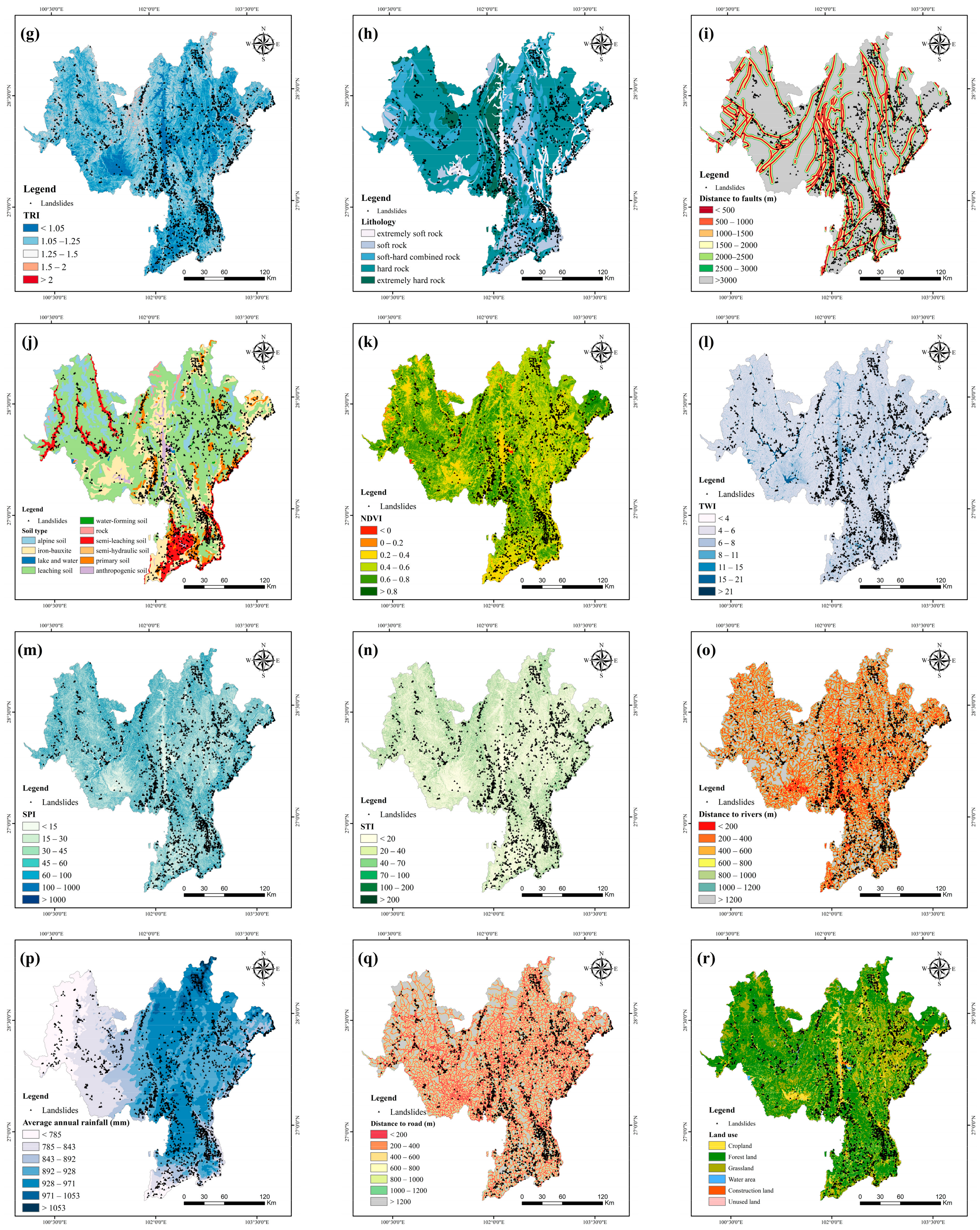
2.3. Landslide Conditioning Factors

LCFs are predictors for landslide susceptibility modeling and are often referred to as input features in the context of machine learning, which also need to be determined. Because of the extremely complicated formation mechanism of landslides, there is currently still no clear guide for the selection of LCFs [51]. Following the previous literature and considering the local characteristics of the study area and the issue of data availability [6,25], we selected 18 LCFs in 5 categories: topography, geology, ecology, hydrology and meteorology, and human activity.

Table 2. The conditioning factors and their data sources.

Category	Conditioning Factor	Data Name	Data Source	Data Type	Precision
Topography factors	Elevation	DEM	Geospatial Data Cloud	Grid	30 m
	Slope angle
	Slope aspect
	Profile curvature
	Plan curvature
	Topographic relief
	Topographic roughness index
Geology factors	Lithology	Geologic map	RESDC	Vector	1:200,000
	Distance to faults
Ecology factors	Soil type	Soil map		Grid	30 m
	Normalized difference vegetation index	Landsat8	United States Geological Survey	Grid	30 m
Hydrology and meteorology factors	Topographic wetness index	DEM	Geospatial Data Cloud	Grid	30 m
	Stream power index
	Sediment transport index
	Distance to rivers	River map	National Basic Geographical Database (NBGD)	Vector	1:250,000
	Average annual rainfall	Rainfall monitoring data	China Meteorological Data Network	Tabular	-
Human activity factors	Distance to roads	Road map	NBGD	Vector	1:250,000
	Land use	Land use map	RESDC	Grid	30 m

lists the 18 LCFs and their corresponding data sources.

Before the information extraction for these LCFs, we needed to first determine the mapping unit, which not only influences the data preparation process of the factors but also has a significant influence on LSA [43]. A mapping unit is the minimum spatial unit for LSA. We needed to split the study area into many units, and for each unit, we needed to compute the values for its factors and produce its landslide susceptibility value. There are different types of mapping units for LSA, such as grid units, slope units, terrain units, and watershed units [52]. We selected grid units, which are among the most commonly used mapping units for susceptibility evaluation, for LSA in this paper [53]. Specifically, we set the grid size to 90 × 90 m to take into account both accuracy and computational cost.

Accordingly, we needed to compute the values of the 18 LCFs for each grid. The computation process consisted of three steps. First, we collected all the necessary datasets, from which the information of the 18 LCFs was extracted. Second, we applied the reclassification operation to the continuous variables. The extracted information has different nominal scales. For example, elevation and slope angle are continuous variables, and land use and soil type have categorical scales, while lithology is an ordinal variable. These differences in the nominal scales of the factors may lead to some uncertainty in ML models due to data discretization [25]. Therefore, we reclassified continuous variables into discrete ones by learning from the classification strategies of existing studies [45,46].

Table 3. Classification of landslide conditioning factors.

Category	Factor	Classification Scheme
Topography factors	Elevation (m)	1. <1500; 2. 1500–2000; 3. 2000–2500; 4. 2500–3000; 5. 3000–3500; 6. 3500–4000; 7. >4000
	Slope angle (°)	1. <10; 2. 10–20; 3. 20–30; 4. 30–40; 5. 40–50; 6. >50
	Slope aspect	1. flat; 2. north; 3. northeast; 4. east; 5. southeast; 6. south; 7. southwest; 8. west; 9. northwest
	Profile curvature	1. <−3; 2. −3 to −2; 3. −2 to −1; 4. −1 to 0; 5. 0 to 1; 6. 1 to 2; 7. 2 to 3; 8. >3
	Plan curvature	1. <−2; 2. −2 to −1; 3. −1 to −0.5; 4. −0.5 to 0; 5. 0 to 0.5; 6. 0.5 to 1; 7. 1 to 2; 8. >2
	Topographic relief (m)	1. <20; 2. 20–35; 3. 35–50; 4. 50–65; 5. 65–80; 6. 80–110; 7. >110
	Topographic roughness index	1. <1.05; 2. 1.05–1.25; 3. 1.25–1.5; 4. 1.5–2; 5. >2
Geology factors	Lithology	1. extremely soft rock; 2. soft rock; 3. soft–hard combined rock; 4. hard rock; 5. extremely hard rock
	Distance to faults (m)	1. <500; 2. 500–1000; 3. 1000–1500; 4. 1500–2000; 5. 2000–2500; 6. 2500–3000; 7. >3000
Ecology factors	Soil type	1. semi-leaching soil; 2. semi-hydraulic soil; 3. primary soil; 4. alpine soil; 5. lake and water; 6. leaching soil; 7. anthropogenic soil; 8. water-forming soil; 9. iron-bauxite; 10. rock
	Normalized difference vegetation index	1. <0; 2. 0–0.2; 3. 0.2–0.4; 4. 0.4–0.6; 5. 0.6–0.8; 6. >0.8
Hydrology and meteorology factors	Topographic wetness index	1. <4; 2. 4–6; 3. 6–8; 4. 8–11; 5. 11–15; 6. 15–21; 7. >21
	Stream power index	1. <15; 2. 15–30; 3. 30–45; 4. 45–60; 5. 60–100; 6. 100–1000; 7. >1000
	Sediment transport index	1. <20; 2. 20–40; 3. 40–70; 4. 70–100; 5.100–200; 6. >200
	Distance to rivers (m)	1. <200; 2. 200–400; 3. 400–600; 4. 600–800; 5. 800–1000; 6. 1000–1200; 7. >1200
	Average annual rainfall (mm)	1. <785; 2. 785–843; 3. 843–892; 4. 892–928; 5. 928–971; 6. 971–1053; 7. >1053
Human activity factors	Distance to roads (m)	1. <200; 2. 200–400; 3. 400–600; 4. 600–800; 5. 800–1000; 6. 1000–1200; 7. >1200
	Land use	1. cropland; 2. forest land 3. grassland; 4. water area; 5. construction land; 6. unused land

presents the classification scheme of each factor. Third, we uniformly converted the data of the 18 LCFs into grids with a 90 m resolution (Figure 2). In addition, in order to avoid the impact of differences between different orders of magnitude on the model, all conditioning factors were normalized to 0–1 before being injected into the model. In the following subsections, we present the specific data extraction methods for each factor and their relevance to landslides, i.e., the reasons why they can influence landslide occurrence.

2.3.1. Topography Factors

The topography factors include elevation (Figure 2a), slope angle (Figure 2b), slope aspect (Figure 2c), profile curvature (Figure 2d), plan curvature (Figure 2e), topographic relief (Figure 2f), and topographic roughness index (TRI) (Figure 2g). They were all calculated from DEM data (ASTER GDEM V3.0 from the Geospatial Data Cloud (http://www.gscloud.cn/, accessed on 27 July 2022)) using ArcGIS software. They were reclassified into different numbers of categories: 7 for elevation, 6 for slope angle, 9 for slope aspect, 8 for profile curvature and plan curvature, 7 for topographic relief, and 5 for TRI.

Elevation is a very common factor in landslide susceptibility evaluation [5], and it affects landslides mainly by influencing the distribution of other factors, such as vegetation, climate, water systems, and human activities [46]. Slope angle is a key factor affecting the stability of a slope [54]. It has a significant impact on the distribution of the slope stress field, the surface runoff process, and the accumulation of slope sediment, which are closely related to the occurrence of landslides [55]. Slope aspect is also relevant to slope stability by affecting solar radiation and rainfall seepage [56]. Profile curvature and plan curvature are two proxies of surface curvature, and they can, respectively, affect the deceleration and acceleration of surface water flow and the divergence and convergence of water flow, which in turn contributes to deposition and erosion [57]. Topographic relief reflects the displacement potential energy of the slope material [31], influencing the frequency and scale of landslide occurrences. TRI is the degree of soil surface depression, representing the change in surface erosion [58].

2.3.2. Geology Factors

Lithology (Figure 2h) and distance to faults (Figure 2i) were selected as geological factors. They were extracted from a geological map of the RESDC. While there are multiple distance measures, we specifically selected the Euclidean distance for distance to faults. The computation was implemented by applying the Euclidean Distance tool from ArcGIS Toolboxes to the geological map. We reclassified distance to faults into 7 categories.

Lithology can directly affect the strength of rock and plays a key role in the development of landslides [59]. In geology, lithology is often represented using engineering rock groups [60]. By merging strata with similar mechanical properties in the study area, the engineering rock groups can be divided into five categories: extremely hard rock, hard rock, soft–hard combined rock, soft rock, and extremely soft rock. Distance to faults can change landslides’ susceptibility due to its influence on the degree of weathering and fracturing of the rock [61].

2.3.3. Ecology Factors

Soil type (Figure 2j) and the normalized difference vegetation index (NDVI) (Figure 2k) were used as proxies of ecological factors. Soil type data were obtained from RESDC. NDVI value can change over time all year around because of seasonal fluctuations. Therefore, we computed NDVI data as the average NDVI calculated using Landat8 images from 2015 to 2019, and images were downloaded from the United States Geological Survey website (https://www.usgs.gov/, accessed on 27 July 2022). NDVI was reclassified into 6 categories.

Different soil types differ in soil water content and viscosity, which may affect the surface sliding [59]. Ten soil types are found in the study area: semi-leaching soil, semi-hydraulic soil, primary soil, alpine soil, lake and water, leaching soil, anthropogenic soil, water-forming soil, iron-bauxite, and rock. NDVI reflects the growth status and coverage of vegetation, which have an important impact on slope stability [48].

2.3.4. Hydrology and Meteorology Factors

The topographic wetness index (TWI) (Figure 2l), stream power index (SPI) (Figure 2m), sediment transport index (STI) (Figure 2n), distance to rivers (Figure 2o), and average annual rainfall (Figure 2p) were considered as hydrology and meteorology factors. TWI, SPI, and STI were extracted from the DEM, and they were reclassified into 7, 7, and 6 categories, respectively. Distance to rivers was also computed by applying the Euclidean Distance tool to the river map from the National Basic Geographical Database (https://www.webmap.cn/, accessed on 27 July 2022) and was reclassified into 7 categories. The average annual rainfall was calculated via kriging interpolation based on the rainfall data from 2015 to 2019 obtained from the China Meteorological Data Network (http://www.nmic.cn/, accessed on 27 July 2022) and was also reclassified into 7 categories.

TWI quantifies the spatial distribution of soil hydrology and reflects the role of topography in controlling hydrological processes [62]. SPI measures the erosive capacity of water flow that occurs in landslides. STI represents the amount of sediment transport by water flow in landslides [4]. Distance to rivers is negatively correlated with slope stability [63], meaning that a decrease in this distance can lead to an increase in erosion at the base of the slope and saturation of material on the slope. Average annual rainfall reflects the year-round meteorological conditions in a region and represents the spatial distribution difference in precipitation [59], and an uneven rainfall distribution plays an important role in slope damage induced in specific areas [64].

2.3.5. Human Activity Factors

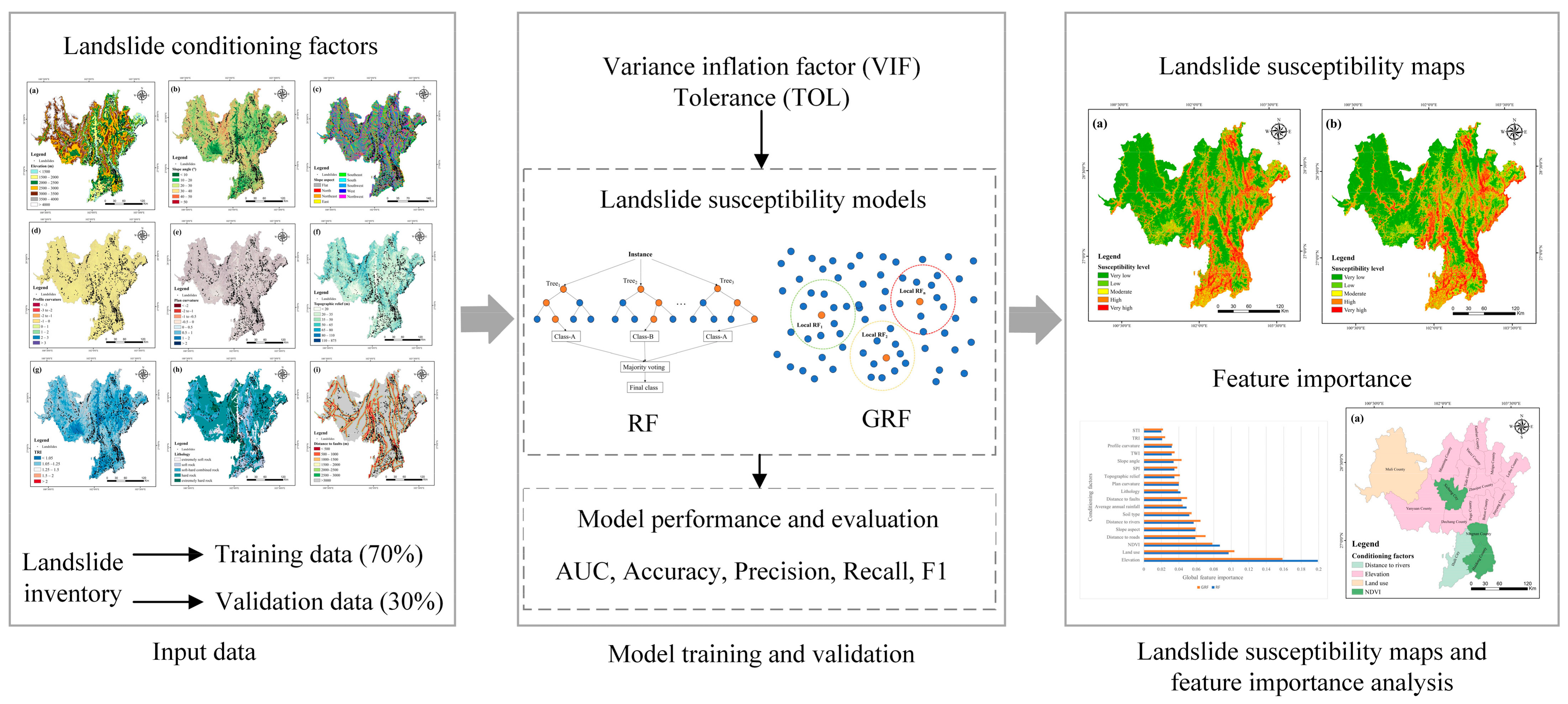
Human activity factors include distance to roads (Figure 2q) and land use (Figure 2r). Distance to roads was computed in the same way as distance to faults using the road map and was reclassified into 7 categories, and land-use data for 2018 were obtained from RESDC.

Road construction can change the original slope conditions. The shorter the distance to roads, the worse the slope stability [48]. Land use represents surface vegetation conditions and can reflect the extent of human interference with slope stability [61]. We considered 6 land-use categories in the study area: cropland, forest land, grassland, water area, construction land, and unused land.

3. Methodology

Figure 3 shows an overview of the methodology used in this study. The input data include the landslide inventory, generated non-landslide points, and LCFs. We first randomly divided the landslide inventory and non-landslide points into two subsets, with 70% for training and 30% for validation [65]. Then, we tested for multicollinearity among features. We conducted experiments to identify landslide and non-landslide points based on RF and GRF, and we evaluated their performance. We finally analyzed the landslide susceptibility maps produced by RF and GRF and their output feature importance. In the following, we present the detailed methods used for the above process.

3.1. Feature Screening Method

The 18 LCFs may not be independent of each other, which can introduce noise and have a negative effect on the model performance [5]. We therefore needed to exclude features with high correlation. Specifically, we employed a multicollinearity test to examine the existence of highly correlated features. Tolerance (TOL) and the variance inflation factor (VIF) are two commonly used indicators to help identify multicollinearity, and they can be computed using the following equations:

$$TOL=1-R_i^2,$$

(1)

$$VIF=\frac{1}{TOL},$$

(2)

where $R_i$ is the coefficient of determination of the regression with conditioning factor $i$ as the dependent variable and the remaining conditioning factors as independent variables. The smaller the TOL, the larger the VIF, indicating a higher degree of multicollinearity among the conditional factors [66]. Generally, if TOL > 0.1 and VIF < 10, the multicollinearity among variables is acceptable and has a negligible effect on LSA [67]. We employed SPSS software to implement the multicollinearity analysis of the 18 LCFs.

3.2. Machine Learning Models

3.2.1. Random Forest

RF is a popular ensemble machine learning model based on a bagging algorithm for both classification and regression tasks. RF is built with a collection of decision trees trained using randomly selected subsets of training data. It can model complex non-linear relationships between variables while tolerating relatively high outliers and noise levels [68], and it has been widely used in landslide susceptibility modeling with fair performance [25]. In addition, RF can output the feature importance to show the difference in contributions of features to predictions. The higher the importance value of a feature, the more it contributes to generating correct predictions. When solving a classification problem (including the binary classification task in this work), the output of RF is the class determined by most trees [69]. In this study, we implemented this model using the scikit-learn package in Python, and it has two major hyperparameters that need to be tuned, namely, n_estimators, which controls the number of trees, and max_features, which controls the number of features considered for node splitting. We used the grid search strategy for hyperparameter tuning. The search space of n_estimators is [10, 600] with an interval of 10, and the search space of max_features is {M, M/2, M/3, ${\log }_{2}M$, $\sqrt{M}$}, where M is the total number of features. Based on the hyperparameter tuning results from the training data, we set n_estimators to 500 and max_features to M. RF is a global and aspatial model; thus, it cannot account for the spatial non-stationarity between conditioning factors and landslides.

3.2.2. Geographical Random Forest

GRF is an extension of RF and can take into account the spatial dependence and spatial heterogeneity of data [33]. The basic idea of GRF is similar to that of geographically weighted regression (GWR) [70], whereby GRF decomposes the global RF model into multiple local sub-models. In other words, for each data point, a local RF model is trained using only its nearby observations. Each local model can output the feature importance to show how the features influence landslide susceptibility in a sub-area. By combining all the local models, we can understand how the impact of each feature varies spatially.

Besides the two hyperparameters n_estimators and max_features for RF, GRF has two new hyperparameters: bandwidth and local.w. Bandwidth determines whether other points belong to nearby observations of the target point. There are two types of bandwidth: fixed bandwidth (defined based on a certain distance) and adaptive bandwidth (determining a certain number of nearest neighbors). We chose adaptive bandwidth in this study as it is commonly used when the spatial distribution density of data points varies greatly, which is consistent with this case. When generating predictions for unknown data points, GRF fuses the outputs of the global and local model by a weighted sum. The weights for the global estimate and local estimate are controlled by local.w. The local estimate is obtained using the closest local model. We implemented the GRF model using the SpatialML package (version: 0.1.4) in R. A grid search was used to tune the above two hyperparameters. The search space of bandwidth is [50, 1000] in intervals of 50, and the search space of local.w is {0.25, 0.50, 0.75, 1}. The search results indicated that the optimal values for bandwidth and local.w are 150 and 0.50, respectively. To ensure a fair comparison between GRF and RF, the same n_estimators and max_features values for RF were used for GRF.

3.3. Model Evaluation Metrics and Validation Methods

We evaluated the models in LSA from two aspects. The first aspect is to evaluate the performances of the models in classifying positive and negative samples in the validation data. Accuracy, precision, recall, F-score, and AUC (area under the curve), which are commonly used for evaluating binary classifiers, were selected to assess the performances of RF and GRF in LSA. The first four metrics were calculated as follows:

$$accuracy=\frac{TP+TN}{TP+FP+TN+FN},$$

(3)

$$precision=\frac{TP}{TP+FP},$$

(4)

$$recall=\frac{TP}{TP+FN},$$

(5)

$$F\text{-}score=\frac{2\times TP}{2\times TP+FP+FN},$$

(6)

where $TP$ (true positives) and $TN$ (true negatives) are the numbers of correctly identified landslides and non-landslides, and $FP$ (false positives) and $FN$ (false negatives) are the numbers of incorrectly identified landslide and non-landslide points.

AUC refers to the area under the receiver operating characteristic (ROC) curve, which is a graphical plot that represents the predictive ability of a binary classifier. In this curve, the horizontal axis represents the false positive rate (FPR), i.e., the ratio of $FP$ to the number of all non-landslide points, and the vertical coordinate indicates the true positive rate (TPR), i.e., the ratio of $TP$ to the number of all landslide points. The higher the AUC value of the ROC curve for a classifier, the better its predictive ability [71].

Random 10-fold cross-validation (CV) and spatial CV were used for computing the above metrics of RF and GRF using the validation data. In the random 10-fold CV, the validation data were randomly divided into 10 parts with equal size. The whole process was iterated 10 times, and in each iteration, 9 parts were used for training and the remaining part was used for testing. The average performance metrics of the 10 iterations are reported as the final performance score of the models. While random 10-fold CV is easy to implement, it is based on the assumption that the samples are independent of each other. However, LSA has a significant nature of spatial autocorrelation, which violates the basic assumption of random 10-fold CV, possibly leading to a biased model assessment result.

To address such bias, we considered spatial CV, which splits the data into subsets spatially rather than randomly. Through spatial splitting, spatial CV can account for the spatial dependence of data, therefore producing a model performance estimate closer to the truth. Specifically, we used the k-means clustering-based spatial CV method, in which the data were divided into 10 clusters based on the spatial coordinates of the samples using the k-means clustering algorithm. The validation process also consisted of 10 iterations, whereby 9 clusters were used for training, and 1 was used for testing. We implemented this method using the scikit-learn package in Python, and we only need to set the number of clusters to form as 10.

The second aspect is to evaluate the quality of the landslide susceptibility maps using landslide density (LD), whereby the values for each pixel are the probabilities of belonging to landslides output by the trained models. We classified all pixels into 5 categories using the natural breaks method based on their susceptibility: very low, low, moderate, high, and very high. We did not use the quantile method for classifying the susceptibility maps for two reasons. First, when using 1:1 ratio of landslide points to non-landslide points (which is the case of this paper), the existing studies mostly used the natural breaks method for classifying landslide susceptibility maps, while the quantile method was used less. Second, if the quantile method is used for the classification, the areas of each landslide susceptibility level in the maps should be the same, which has a great impact on calculating the landslide density. The map quality can be assessed by calculating LD of each class [72,73], which is defined by the following equation:

$$L{D}_i=\frac{L{P}_i}{A{P}_i},$$

(7)

where $L{D}_i$ is the landslide density of class $i$, $L{P}_i$ is the ratio of the number of landslide points in all the pixels of class $i$ to the total number of landslide points, and $A{P}_i$ is the ratio of the area of pixels belonging to class $i$ to the total area.

4. Results

4.1. Multicollinearity Diagnosis

Table 4. Multicollinearity analysis of conditioning factors.

Conditioning Factors	TOL	VIF	Conditioning Factors	TOL	VIF
Elevation	0.59	1.70	Soil type	0.82	1.23
Slope angle	0.15	6.56	NDVI	0.87	1.16
Slope aspect	0.99	1.01	TWI	0.49	2.06
Profile curvature	0.77	1.30	SPI	0.31	3.26
Plan curvature	0.60	1.67	STI	0.35	2.83
Topographic relief	0.17	5.74	Distance to rivers	0.86	1.16
TRI	0.23	4.31	Average annual rainfall	0.80	1.25
Lithology	0.91	1.10	Distance to roads	0.87	1.14
Distance to faults	0.95	1.05	Land use	0.94	1.06

shows the results of the multicollinearity analysis of the 18 LCFs. As can be seen, the TOL values of all conditioning factors are higher than 0.1, and the VIF values are lower than 10, indicating low multicollinearity among them. We therefore used all conditioning factors in the subsequent landslide susceptibility modeling.

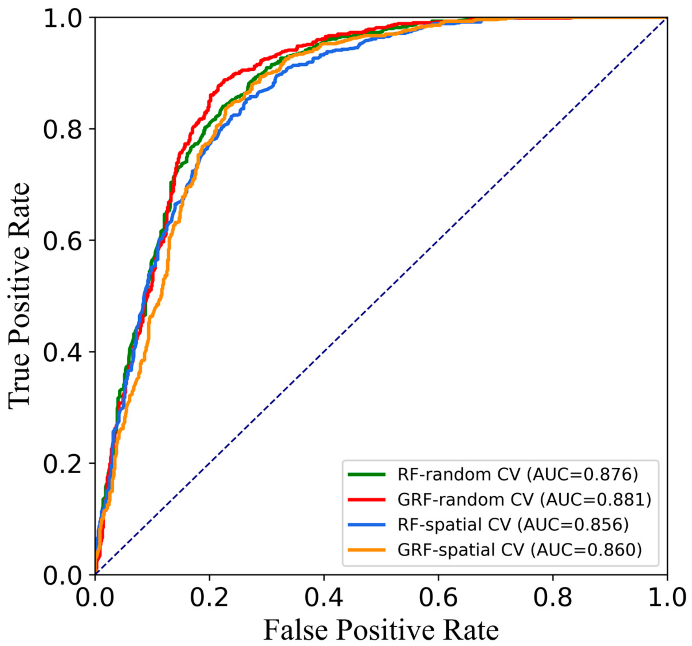
4.2. Model Performance Evaluation

Table 5. Performances of RF and GRF on the validation data using random CV and spatial CV.

Model	Cross-Validation Method	Accuracy	Precision	Recall	F-Score	AUC
RF	Random CV	0.806	0.781	0.852	0.815	0.876
GRF		0.829	0.801	0.879	0.838	0.881
RF	Spatial CV	0.789	0.766	0.833	0.798	0.856
GRF		0.798	0.767	0.858	0.810	0.860

shows the performances of RF and GRF using random CV and spatial CV based on the validation data. AUC was computed based on the ROC curves of RF and GRF shown in Figure 4. As can be seen in Table 5, the highest performance was achieved by GRF when using random CV, with an accuracy of 0.829 and an AUC of 0.881. The four different cases all achieved high recalls (from 0.833 to 0.879), suggesting that they could find most of the landslide points. In contrast, their precisions were lower than their recalls (from 0.766 to 0.801), indicating that about 20% to 23% of the identified landslide points were incorrect. In either cross-validation strategy, GRF obtained higher performances than RF over all metrics, suggesting that it has stronger capability in distinguishing between landslide and non-landslide points. For example, when using random CV, GRF achieved an increase of 0.02 and 0.03 in precision and recall compared with RF, indicating that GRF can not only effectively exclude non-landslide points, but also successfully recognize more landslide points.

When it comes to using different cross-validation methods, we can observe that the performances of both models using random CV were significantly higher than those based on spatial CV. For example, the F-scores of RF and GRF were 0.815 and 0.838 for random CV, which were 0.02 and 0.03 higher than those of spatial CV. This piece of evidence strongly shows that random CV can lead to a biased over-optimistic model performance estimate due to its lack of consideration of the spatial dependence among the spatial data. In contrast, spatial CV can resolve such bias by splitting the data into subsets spatially instead of randomly. Furthermore, when using random CV, the increases for GRF over RF in the five metrics were 0.02, 0.02, 0.03, 0.02, and 0.01. Such increases based on spatial CV, however, were reduced: 0.01, 0, 0.03, 0.01, and 0. In other words, the performance differences between GRF and RF based on spatial CV were significantly narrowed. This second piece of evidence suggests that more complex models (i.e., GRF in this study) are more likely to achieve a higher performance when using random CV than simple models (i.e., RF in this study). Spatial CV can help, to a certain extent, to reduce the tendency of selecting more complex models.

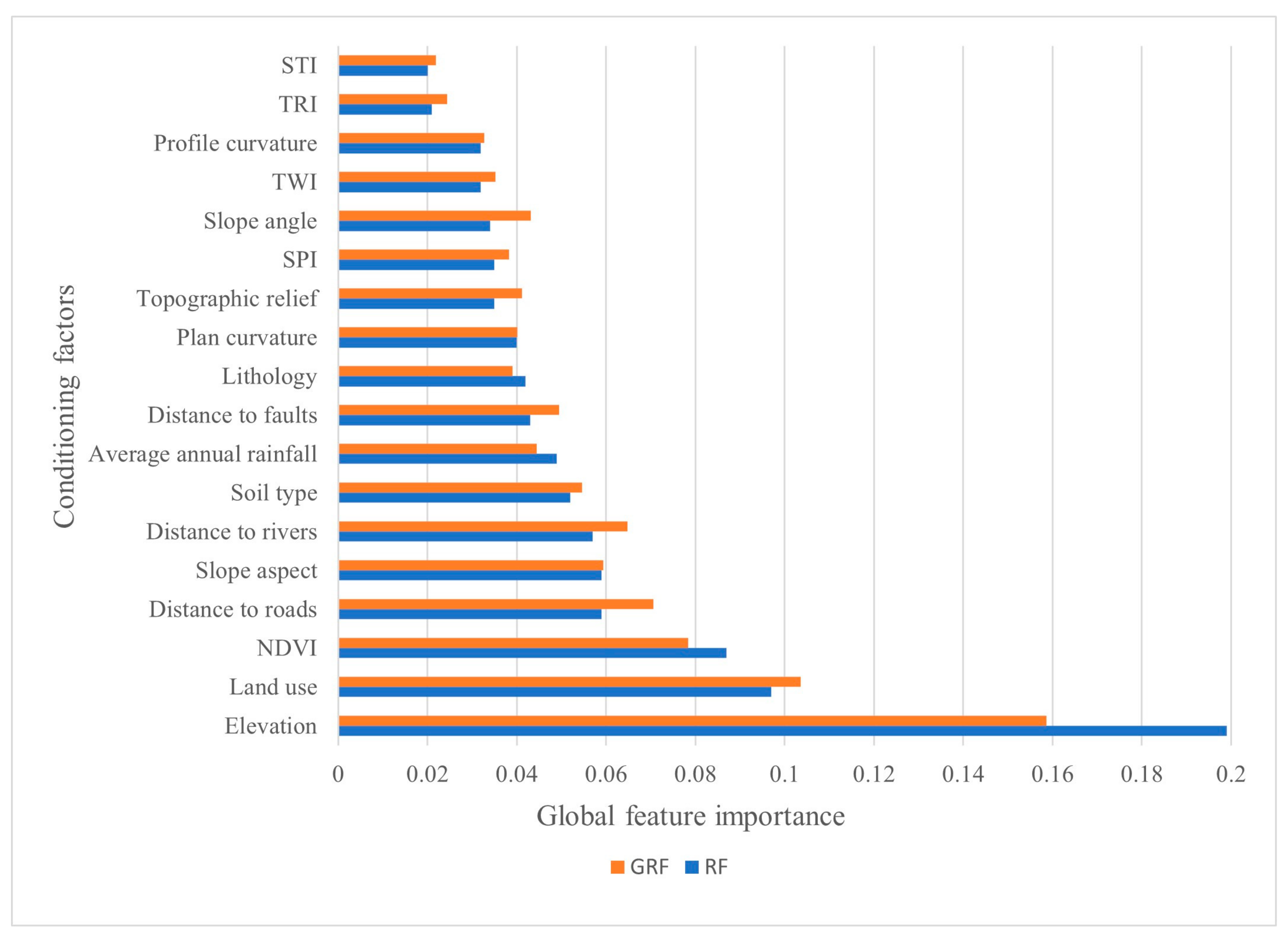
4.3. Global Feature Importance Comparison

The global feature importance of each conditioning factor based on RF and GRF is depicted in Figure 5. The feature importance for RF can be directly obtained from the trained model, while the global feature importance for GRF is computed as the average of the local feature importance output by all the local models. Generally, the rankings of the feature importance were very similar. For example, they had the same four most important factors, namely, elevation, land use, NDVI, and distance to roads, and their four least important factors were also the same, namely, STI, TRI, profile curvature, and TWI.

Apart from that, some differences between them could still be observed. Though elevation was the most important factor for both models, it had a higher importance value for RF than GRF, by 0.04. Slope aspect and distance to rivers were ranked the fifth and sixth most important features in RF, while they had the opposite rankings for GRF. The fifth least important features for RF and GRF were slope angle and SPI, respectively, differing from the findings in the previous literature [14]. The possible reason is that these features were computed based on elevation, and they may be less important since elevation already explained the output for both of them. Two other factors with very different rankings were slope angle, ranked 14th for RF and 10th for GRF, and lithology, ranked 10th for RF and 14th for GRF. The importance rankings of the remaining features, such as average annual rainfall, distance to faults, and topographic relief, generally differed by only one place.

While RF and GRF generally obtained quite similar importance rankings, GRF can learn the local feature importance and show how it varies spatially. We discuss the local patterns of the feature importance in Section 5.1.

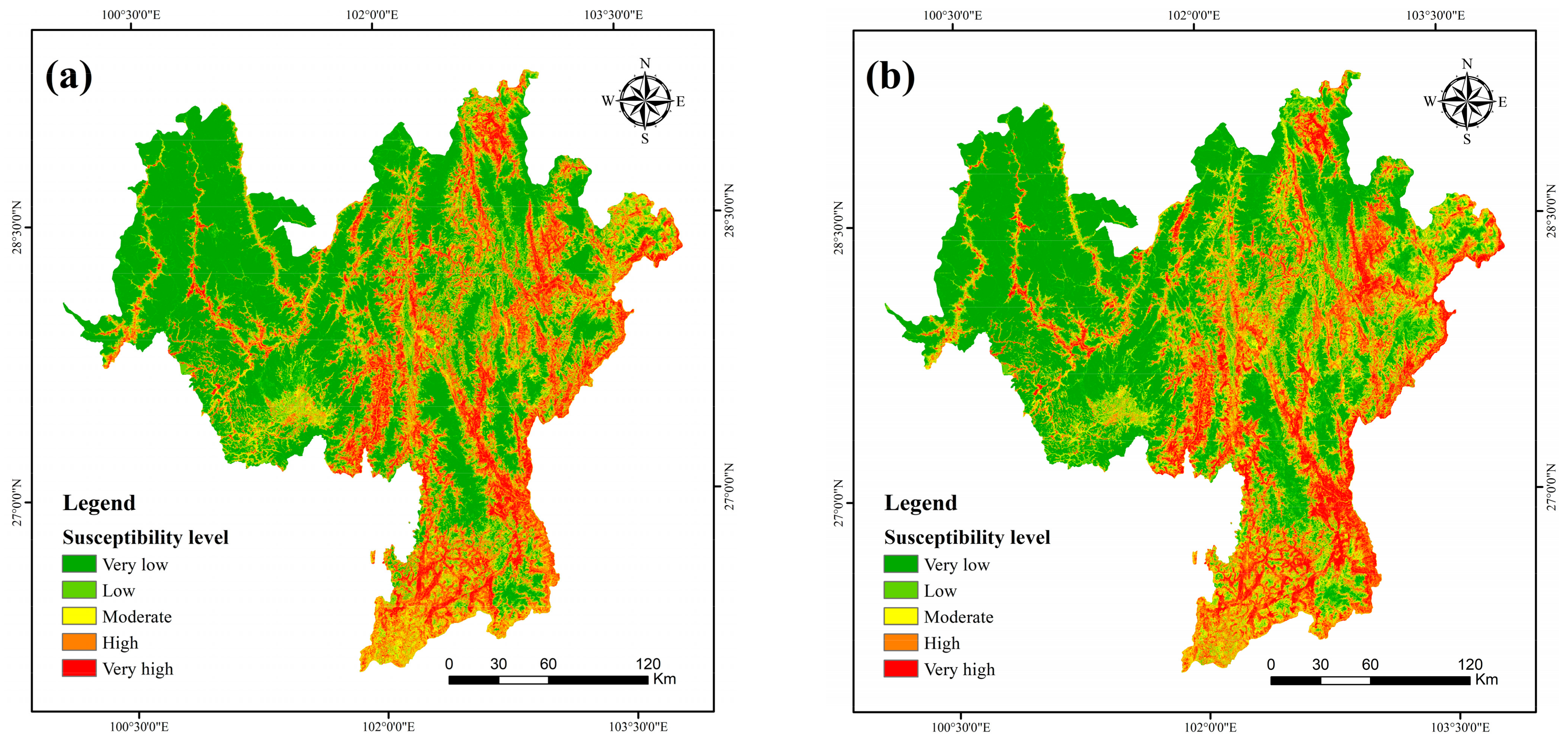
4.4. Landslide Susceptibility Maps

The trained RF and GRF models were employed to predict the landslide susceptibility for the entire study area. We then leveraged the natural breaks method in ArcGIS software to classify the computed landslide susceptibility into five levels: very low, low, moderate, high, and very high, thereby producing the landslide susceptibility maps (Figure 6). Overall, the two models showed a similar spatial distribution. The high-risk areas are concentrated in the southern and eastern areas, which is consistent with the report on key prevention areas for geological hazards published by the Liangshan government (http://www.lsz.gov.cn/xxgk/zcwj/zzfbgsh/202206/t20220610_2238890.html, accessed on 27 July 2022). The areas with very low susceptibility are located in the western part.

In order to quantitatively analyze the differences between the two susceptibility maps, we further computed the area of each susceptibility level and the number of landslide points for each level, and we calculated the landslide density. The results are shown in

Table 6. Evaluation results of landslide susceptibility maps.

Models	Susceptibility Level	Area (km2)	Percentage of Area (%)	Number of Landslides	Percentage of Landslides (%)	Landslide Density
RF	Very Low	26,450.31	43.86	12	0.52	0.01
	Low	10,132.89	16.80	61	2.64	0.16
	Moderate	8327.19	13.81	184	7.96	0.58
	High	8239.20	13.66	469	20.29	1.48
	Very High	7154.91	11.86	1586	68.60	5.78
GRF	Very Low	24,289.59	40.28	8	0.35	0.01
	Low	11,706.39	19.41	31	1.34	0.07
	Moderate	8964.90	14.87	138	5.97	0.40
	High	8349.93	13.85	411	17.78	1.28
	Very High	6993.69	11.60	1724	74.57	6.43

. As can be seen, the areas of regions with a very high level and high level are quite similar for RF and GRF. The area with a very high level for GRF is 0.26% smaller than that for RF, while the area with a high level for GRF is 0.19% larger than that for RF. Meanwhile, the areas with very low and low-level regions are fairly different, with a gap of 3.58% and 2.61%, respectively. In terms of the landslide points for each level, GRF showed a significantly better performance, with 92.35% of the landslide points correctly identified as grids with high and very high susceptibility levels and only 1.69% of them incorrectly identified as grids with very low and low susceptibility levels. In contrast, RF could only correctly consider 88.89% of the landslide points as high and very high susceptibility grids, while it incorrectly considered 3.16% of them as very low and low susceptibility grids. Similarly, GRF achieved a higher landslide density for the high and very high levels, and a lower landslide density for the very low and low levels, compared to RF. The differences between GRF and RF in the percentage of landslides and landslide density suggest that GRF is better at distinguishing areas with a high risk and areas with a low risk, which is very important for the local government to prevent potential hazards.

5. Discussion

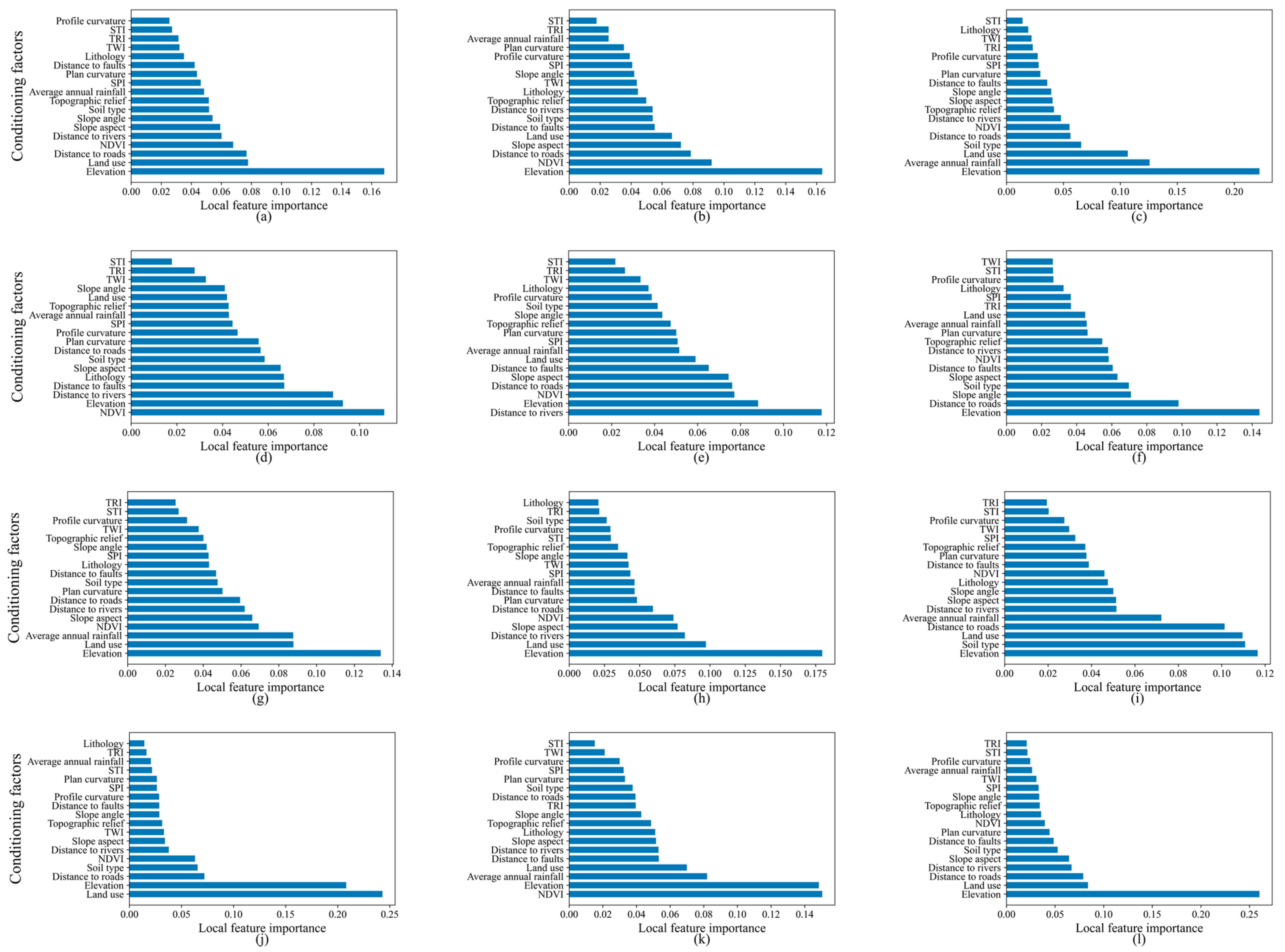
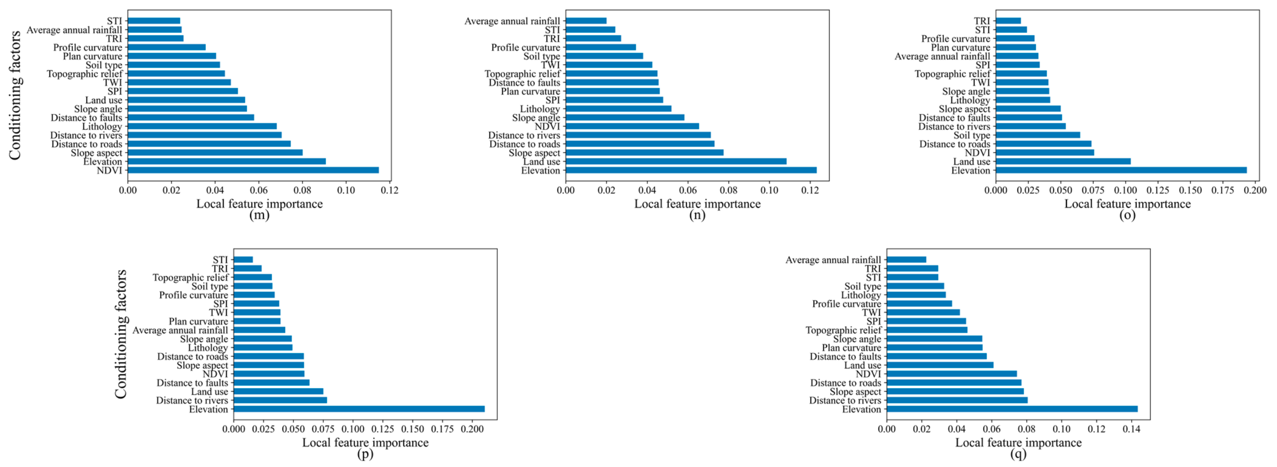
5.1. Local Feature Importance

To understand how the influence of LCFs on LSA varies spatially, we computed the feature importance for each county in Liangshan by averaging the feature importance derived from all the local models within each county, as shown in Figure 7. As can be seen, in comparison with the similar global feature importance rankings of RF and GRF, the rankings of the local feature importance were largely different for each county. For most of the counties, elevation, NDVI, distance to rivers, and land use were ranked among the top five most important features, which were precisely the top four most important features suggested by the global feature importance of RF and GRF. Beyond this, some other features also appeared among the top five most important features for some counties: for example, average annual rainfall for the counties of Ganluo, Leibo, Mianning, and Ningnan; soil type for the counties of Ganluo, Jinyang, Mianning, Muli, and Yanyuan; and distance to faults for the counties of Huidong, Ningnan, and Yuexi. STI was the least important feature for seven counties, and TRI was the least important feature for four counties. They were also two of the four least important factors shown in the global feature importance. Some of the features varied greatly in the importance ranking across counties. For example, average annual rainfall was ranked the second most important feature for Ganluo County, while it was ranked the least important feature for the counties of Xide and Zhaojue.

We further mapped the top four most important features of all the counties (Figure 8). Elevation was ranked the most important feature for 12 counties, while the most important feature was NDVI for the counties of Huidong, Ningnan, and Xichang, distance to rivers for Huili City, and land use for Muli County. Nonetheless, elevation was ranked the second most important feature for these five counties. Therefore, elevation has the most significant capacity to distinguish landslide and non-landslide points in Liangshan. Land use was ranked the second most important feature for six counties. The third most important features tended to be distributed across counties, and the maximum number of counties that one feature (i.e., distance to roads) occupied was just four. Distance to roads was also ranked the fourth most important feature for six counties. The differences in the importance ranking of local features in each county indicate that conditioning factors are spatially heterogeneous in predicting landslide occurrence. Therefore, these factors should be given different levels of attention by each county in landslide hazard prevention and mitigation. For example, the Muli County government should focus on the land use of local areas with a high risk, while Huili City should place more focus on risk areas with a shorter distance to rivers.

5.2. Limitations

This study achieved higher performances in LSA using GRF with its good consideration of the spatial heterogeneity among variables and accurately examined the spatial variation in the feature importance. Nevertheless, it remains limited in two aspects. From the perspective of input data, conditioning factors were extracted from datasets with different data types and resolutions or precisions. In order to attain a unified mapping unit, we converted them to grids with a 90 m resolution, which may lead to some uncertainties. One way to solve this problem is to first determine the mapping unit of LSA and collect data with the same resolution as the mapping unit. However, there is often a lack of data that can satisfy the requirement.

Some limitations also exist in the methodological part. First, the computational complexity of GRF is very large due to its need to train many local models. Therefore, the hyperparameter tuning and model training processes are very time-consuming. This issue can be mitigated to some extent through the use of more powerful hardware and parallel implementations of local model computation. Second, according to Tobler’s first law of geography, everything is related to everything else, but closer things are more related to each other than distant things. This can also be interpreted as the distance decay effect of the spatial dependence among spatial objects, i.e., the dependence among objects decreases as their distance increases. However, the GRF implementation that we used was based on the assumption that the spatial dependence between the nearby observations and the target data point is constant in terms of distance and did not consider the distance decay effect. We have noted that the latest implementation of GRF incorporates a new parameter, “weighted”, which allows the model to assign different weights to observations based on their distances. This can help take into account the distance decay effect of spatial dependence, thereby producing more accurate estimates. Third, the map for inventory data showed an incomplete bias in terms of the spatial distribution of landslide points across the study area. For example, landslide points are very dense in the south, while they are sparse in the northwest. Previous studies have shown that the landslide susceptibility maps generated using incomplete landslide inventory data can be biased [74,75]. However, GRF cannot fully address such an issue, which may further lead to a bias of local effects captured by GRF. For example, for a sub-area with dense data records, more local GRF models will be built and trained, thereby better showing the local effects. In contrast, for sub-areas with sparse data records, GRF can only capture the spatial dependence among data on a larger scale since only a smaller number of local models can be trained. Steger et al. suggested that the use of non-linear mixed-effect models can partially address the propagation of the bias [76]. We should try these models to deal with the data incompleteness in the future.

6. Conclusions

Landslides have great destructive power and can pose a serious threat to the safety of people’s lives and property, the social economy, and the ecological environment. At present, however, few studies have modeled LSA considering the spatial heterogeneity of landslides. In this work, we employed GRF, a spatially explicit model that can address the spatial variation in landslide modeling, to assess landslide susceptibility in Liangshan Prefecture, China. We evaluated the performances of GRF and RF using not only random CV but also spatial CV, which can help split data into subsets by accounting for the spatial dependence among the data. We also discussed the global and local feature importance derived from RF and GRF. Ultimately, we came to the following conclusions. First, GRF succeeds in considering the spatial heterogeneity among variables, thereby achieving a higher performance than RF, with an AUC of 0.86 in LSA based on spatial CV. Second, spatial CV divides data into subsets spatially and can effectively resolve the over-optimistic bias in model performance evaluation brought by the random split of random CV. Third, GRF can produce a landslide susceptibility map with a higher quality. Although the landslide susceptibility maps produced by RF and GRF showed a similar spatial distribution, GRF correctly placed 92.35% of the landslide points in high-susceptibility areas. In contrast, RF assigned 88.89% of the landslide points to the correct high-risk areas. The strong capability of GRF in correctly distinguishing high-risk areas and low-risk areas can greatly support the decision making of local governments. Fourth, GRF can effectively investigate how the feature importance varies across counties and identify which features contribute more locally to landslides, thereby providing insights and scientific suggestions to local governments on landslide control and management.

Although this study is not the first to use GRF for LSA, it is unique in that we assessed the model performance with spatial CV, addressing the biased model error evaluation, and analyzed the differences in the local feature importance of the conditioning factors. In addition, while this study has its limitations, it improves our understanding of spatially varying relationships between conditioning factors and landslide susceptibility.

Two directions can be pursued in the near future. First, we can continue to improve the implementation of GRF. For example, we could implement local model training in a parallel manner, thereby improving the running efficiency. Second, some other spatially explicit machine learning models have recently emerged, such as geographically weighted support vector machines and geographically weighted artificial neural networks, which have not yet been applied in landslide susceptibility modeling. We can attempt to apply them and determine the most effective model by comparing their performances in LSA.

References

1. Rotaru, A.; Oajdea, D.; Răileanu, P. Analysis of the Landslide Movements. Int. J. Geol. 2007, 1, 70–79. [Google Scholar]
2. Dai, F.C.; Lee, C.F.; Ngai, Y.Y. Landslide Risk Assessment and Management: An Overview. Eng. Geol. 2002, 64, 65–87. [Google Scholar] [CrossRef]
3. Niu, C.; Zhang, H.; Liu, W.; Li, R.; Hu, T. Using a Fully Polarimetric SAR to Detect Landslide in Complex Surroundings: Case Study of 2015 Shenzhen Landslide. ISPRS J. Photogramm. Remote Sens. 2021, 174, 56–67. [Google Scholar] [CrossRef]
4. Fang, Z.; Wang, Y.; Peng, L.; Hong, H. A Comparative Study of Heterogeneous Ensemble-Learning Techniques for Landslide Susceptibility Mapping. Int. J. Geogr. Inf. Sci. 2021, 35, 321–347. [Google Scholar] [CrossRef]
5. Chen, W.; Zhang, S.; Li, R.; Shahabi, H. Performance Evaluation of the GIS-Based Data Mining Techniques of Best-First Decision Tree, Random Forest, and Naïve Bayes Tree for Landslide Susceptibility Modeling. Sci. Total Environ. 2018, 644, 1006–1018. [Google Scholar] [CrossRef]
6. Reichenbach, P.; Rossi, M.; Malamud, B.D.; Mihir, M.; Guzzetti, F. A Review of Statistically-Based Landslide Susceptibility Models. Earth-Sci. Rev. 2018, 180, 60–91. [Google Scholar] [CrossRef]
7. Thi Ngo, P.T.; Panahi, M.; Khosravi, K.; Ghorbanzadeh, O.; Kariminejad, N.; Cerda, A.; Lee, S. Evaluation of Deep Learning Algorithms for National Scale Landslide Susceptibility Mapping of Iran. Geosci. Front. 2021, 12, 505–519. [Google Scholar] [CrossRef]
8. Kjekstad, O.; Highland, L. Economic and Social Impacts of Landslides. In Landslides—Disaster Risk Reduction; Sassa, K., Canuti, P., Eds.; Springer: Berlin/Heidelberg, Germany, 2009; pp. 573–587. ISBN 978-3-540-69970-5. [Google Scholar]
9. Yong, C.; Jinlong, D.; Fei, G.; Bin, T.; Tao, Z.; Hao, F.; Li, W.; Qinghua, Z. Review of Landslide Susceptibility Assessment Based on Knowledge Mapping. Stoch. Environ. Res. Risk Assess. 2022, 36, 2399–2417. [Google Scholar] [CrossRef]
10. Lima, P.; Steger, S.; Glade, T.; Murillo-García, F.G. Literature Review and Bibliometric Analysis on Data-Driven Assessment of Landslide Susceptibility. J. Mt. Sci. 2022, 19, 1670–1698. [Google Scholar] [CrossRef]
11. Aditian, A.; Kubota, T.; Shinohara, Y. Comparison of GIS-Based Landslide Susceptibility Models Using Frequency Ratio, Logistic Regression, and Artificial Neural Network in a Tertiary Region of Ambon, Indonesia. Geomorphology 2018, 318, 101–111. [Google Scholar] [CrossRef]
12. Riaz, M.T.; Basharat, M.; Brunetti, M.T. Assessing the Effectiveness of Alternative Landslide Partitioning in Machine Learning Methods for Landslide Prediction in the Complex Himalayan Terrain. Prog. Phys. Geogr. Earth Environ. 2022, 03091333221113660. [Google Scholar] [CrossRef]
13. Regmi, N.R.; Giardino, J.R.; Vitek, J.D. Modeling Susceptibility to Landslides Using the Weight of Evidence Approach: Western Colorado, USA. Geomorphology 2010, 115, 172–187. [Google Scholar] [CrossRef]
14. Quevedo, R.P.; Maciel, D.A.; Uehara, T.D.T.; Vojtek, M.; Rennó, C.D.; Pradhan, B.; Vojteková, J.; Pham, Q.B. Consideration of Spatial Heterogeneity in Landslide Susceptibility Mapping Using Geographical Random Forest Model. Geocarto Int. 2021, 37, 1–24. [Google Scholar] [CrossRef]
15. Zeng, H.; Zhu, Q.; Ding, Y.; Hu, H.; Chen, L.; Xie, X.; Chen, M.; Yao, Y. Graph Neural Networks with Constraints of Environmental Consistency for Landslide Susceptibility Evaluation. Int. J. Geogr. Inf. Sci. 2022, 36, 1–26. [Google Scholar] [CrossRef]
16. Stamatopoulos, C.A.; Di, B. Analytical and Approximate Expressions Predicting Post-Failure Landslide Displacement Using the Multi-Block Model and Energy Methods. Landslides 2015, 12, 1207–1213. [Google Scholar] [CrossRef]
17. Chen, T.; Niu, R.; Jia, X. A Comparison of Information Value and Logistic Regression Models in Landslide Susceptibility Mapping by Using GIS. Environ. Earth Sci. 2016, 75, 867. [Google Scholar] [CrossRef]
18. Vakhshoori, V.; Zare, M. Landslide Susceptibility Mapping by Comparing Weight of Evidence, Fuzzy Logic, and Frequency Ratio Methods. Geomat. Nat. Hazards Risk 2016, 7, 1731–1752. [Google Scholar] [CrossRef]
19. Li, L.; Lan, H.; Guo, C.; Zhang, Y.; Li, Q.; Wu, Y. A Modified Frequency Ratio Method for Landslide Susceptibility Assessment. Landslides 2017, 14, 727–741. [Google Scholar] [CrossRef]
20. Goetz, J.N.; Brenning, A.; Petschko, H.; Leopold, P. Evaluating Machine Learning and Statistical Prediction Techniques for Landslide Susceptibility Modeling. Comput. Geosci. 2015, 81, 1–11. [Google Scholar] [CrossRef]
21. Pourghasemi, H.R.; Rahmati, O. Prediction of the Landslide Susceptibility: Which Algorithm, Which Precision? CATENA 2018, 162, 177–192. [Google Scholar] [CrossRef]
22. Riaz, M.T.; Basharat, M.; Pham, Q.B.; Sarfraz, Y.; Shahzad, A.; Ahmed, K.S.; Ikram, N.; Waseem, M.H. Improvement of the Predictive Performance of Landslide Mapping Models in Mountainous Terrains Using Cluster Sampling. Geocarto Int. 2022, 37, 12294–12337. [Google Scholar] [CrossRef]
23. Huang, F.; Cao, Z.; Guo, J.; Jiang, S.-H.; Li, S.; Guo, Z. Comparisons of Heuristic, General Statistical and Machine Learning Models for Landslide Susceptibility Prediction and Mapping. CATENA 2020, 191, 104580. [Google Scholar] [CrossRef]
24. Dou, J.; Yunus, A.P.; Tien Bui, D.; Merghadi, A.; Sahana, M.; Zhu, Z.; Chen, C.-W.; Khosravi, K.; Yang, Y.; Pham, B.T. Assessment of Advanced Random Forest and Decision Tree Algorithms for Modeling Rainfall-Induced Landslide Susceptibility in the Izu-Oshima Volcanic Island, Japan. Sci. Total Environ. 2019, 662, 332–346. [Google Scholar] [CrossRef] [PubMed]
25. Sun, D.; Shi, S.; Wen, H.; Xu, J.; Zhou, X.; Wu, J. A Hybrid Optimization Method of Factor Screening Predicated on GeoDetector and Random Forest for Landslide Susceptibility Mapping. Geomorphology 2021, 379, 107623. [Google Scholar] [CrossRef]
26. Cheng, J.; Dai, X.; Wang, Z.; Li, J.; Qu, G.; Li, W.; She, J.; Wang, Y. Landslide Susceptibility Assessment Model Construction Using Typical Machine Learning for the Three Gorges Reservoir Area in China. Remote Sens. 2022, 14, 2257. [Google Scholar] [CrossRef]
27. He, Q.; Shahabi, H.; Shirzadi, A.; Li, S.; Chen, W.; Wang, N.; Chai, H.; Bian, H.; Ma, J.; Chen, Y.; et al. Landslide Spatial Modelling Using Novel Bivariate Statistical Based Naïve Bayes, RBF Classifier, and RBF Network Machine Learning Algorithms. Sci. Total Environ. 2019, 663, 1–15. [Google Scholar] [CrossRef] [PubMed]
28. Tien Bui, D.; Tuan, T.A.; Klempe, H.; Pradhan, B.; Revhaug, I. Spatial Prediction Models for Shallow Landslide Hazards: A Comparative Assessment of the Efficacy of Support Vector Machines, Artificial Neural Networks, Kernel Logistic Regression, and Logistic Model Tree. Landslides 2016, 13, 361–378. [Google Scholar] [CrossRef]
29. Kavzoglu, T.; Teke, A. Predictive Performances of Ensemble Machine Learning Algorithms in Landslide Susceptibility Mapping Using Random Forest, Extreme Gradient Boosting (XGBoost) and Natural Gradient Boosting (NGBoost). Arab. J. Sci. Eng. 2022, 47, 7367–7385. [Google Scholar] [CrossRef]
30. Yang, W.; Deng, M.; Tang, J.; Luo, L. Geographically Weighted Regression with the Integration of Machine Learning for Spatial Prediction. J. Geogr. Syst. 2022, 1–24. [Google Scholar] [CrossRef]
31. Gu, T.; Li, J.; Wang, M.; Duan, P. Landslide Susceptibility Assessment in Zhenxiong County of China Based on Geographically Weighted Logistic Regression Model. Geocarto Int. 2022, 37, 4952–4973. [Google Scholar] [CrossRef]
32. Yang, Y.; Yang, J.; Xu, C.; Xu, C.; Song, C. Local-Scale Landslide Susceptibility Mapping Using the B-GeoSVC Model. Landslides 2019, 16, 1301–1312. [Google Scholar] [CrossRef]
33. Georganos, S.; Grippa, T.; Niang Gadiaga, A.; Linard, C.; Lennert, M.; Vanhuysse, S.; Mboga, N.; Wolff, E.; Kalogirou, S. Geographical Random Forests: A Spatial Extension of the Random Forest Algorithm to Address Spatial Heterogeneity in Remote Sensing and Population Modelling. Geocarto Int. 2021, 36, 121–136. [Google Scholar] [CrossRef] [Green Version]
34. Grekousis, G.; Feng, Z.; Marakakis, I.; Lu, Y.; Wang, R. Ranking the Importance of Demographic, Socioeconomic, and Underlying Health Factors on US COVID-19 Deaths: A Geographical Random Forest Approach. Health Place 2022, 74, 102744. [Google Scholar] [CrossRef] [PubMed]
35. Quiñones, S.; Goyal, A.; Ahmed, Z.U. Geographically Weighted Machine Learning Model for Untangling Spatial Heterogeneity of Type 2 Diabetes Mellitus (T2D) Prevalence in the USA. Sci. Rep. 2021, 11, 6955. [Google Scholar] [CrossRef]
36. Aguirre-Gutiérrez, J.; Rifai, S.; Shenkin, A.; Oliveras, I.; Bentley, L.P.; Svátek, M.; Girardin, C.A.J.; Both, S.; Riutta, T.; Berenguer, E.; et al. Pantropical Modelling of Canopy Functional Traits Using Sentinel-2 Remote Sensing Data. Remote Sens. Environ. 2021, 252, 112122. [Google Scholar] [CrossRef]
37. Santos, F.; Graw, V.; Bonilla, S. A Geographically Weighted Random Forest Approach for Evaluate Forest Change Drivers in the Northern Ecuadorian Amazon. PLoS ONE 2019, 14, e0226224. [Google Scholar] [CrossRef]
38. Roberts, D.R.; Bahn, V.; Ciuti, S.; Boyce, M.S.; Elith, J.; Guillera-Arroita, G.; Hauenstein, S.; Lahoz-Monfort, J.J.; Schröder, B.; Thuiller, W.; et al. Cross-Validation Strategies for Data with Temporal, Spatial, Hierarchical, or Phylogenetic Structure. Ecography 2017, 40, 913–929. [Google Scholar] [CrossRef] [Green Version]
39. Xiang, X.; Xiao, D. Socioeconomic Development Evaluation for Chinese Poverty-Stricken Counties Using Indices Derived from Remotely Sensed Data. Eur. J. Remote Sens. 2021, 54, 226–239. [Google Scholar] [CrossRef]
40. Liu, B.; Cao, W.; Liu, S.; Tao, H.; Shi, Z.; Guo, S. Land Resources Assessment Model for Mountainous Areas Based on GIS: A Case Study of Liangshan Yizu Autonomous Prefecture, Sichuan Province. Acta Geogr. Sin. 2011, 66, 1131. [Google Scholar] [CrossRef]
41. Ouyang, Y.; Zhang, J.; Liu, H.; Huang, H.; Zhang, T.; Huang, Y. Classification of Soil Parent Materials in Mountain Areas of Southwest China Based on Geological Formations: A Case Study of Daliangshan Region. Geol. Surv. China 2021, 8, 50–62. [Google Scholar] [CrossRef]
42. Jiang, Y.H.; Wei, F.Q.; Zhang, J.H.; Deng, B.; Xu, A.S. Debris Flow and Landslide Forecast Based on Gis and Doppler Weather Radar in Liangshan Prefecture. Ital. J. Eng. Geol. Environ. 2011, 903–911. [Google Scholar] [CrossRef]
43. Wang, Y.; Feng, L.; Li, S.; Ren, F.; Du, Q. A Hybrid Model Considering Spatial Heterogeneity for Landslide Susceptibility Mapping in Zhejiang Province, China. CATENA 2020, 188, 104425. [Google Scholar] [CrossRef]
44. Wei, A.; Yu, K.; Dai, F.; Gu, F.; Zhang, W.; Liu, Y. Application of Tree-Based Ensemble Models to Landslide Susceptibility Mapping: A Comparative Study. Sustainability 2022, 14, 6330. [Google Scholar] [CrossRef]
45. Wang, S.; Zhuang, J.; Mu, J.; Zheng, J.; Zhan, J.; Wang, J.; Fu, Y. Evaluation of Landslide Susceptibility of the Ya’an–Linzhi Section of the Sichuan–Tibet Railway Based on Deep Learning. Environ. Earth Sci. 2022, 81, 250. [Google Scholar] [CrossRef]
46. Zhou, X.; Wen, H.; Zhang, Y.; Xu, J.; Zhang, W. Landslide Susceptibility Mapping Using Hybrid Random Forest with GeoDetector and RFE for Factor Optimization. Geosci. Front. 2021, 12, 101211. [Google Scholar] [CrossRef]
47. Yao, K.; Yang, S.; Wu, S.; Tong, B. Landslide Susceptibility Assessment Considering Spatial Agglomeration and Dispersion Characteristics: A Case Study of Bijie City in Guizhou Province, China. ISPRS Int. J. Geo-Inf. 2022, 11, 269. [Google Scholar] [CrossRef]
48. Yuan, R.; Chen, J. A Hybrid Deep Learning Method for Landslide Susceptibility Analysis with the Application of InSAR Data. Nat. Hazards 2022, 2, 1393–1426. [Google Scholar] [CrossRef]
49. Sun, D.; Wen, H.; Xu, J.; Zhang, Y.; Wang, D.; Zhang, J. Improving Geospatial Agreement by Hybrid Optimization in Logistic Regression-Based Landslide Susceptibility Modelling. Front. Earth Sci. 2021, 9, 686. [Google Scholar] [CrossRef]
50. Yi, Y.; Zhang, W.; Xu, X.; Zhang, Z.; Wu, X. Evaluation of Neural Network Models for Landslide Susceptibility Assessment. Int. J. Digit. Earth 2022, 15, 934–953. [Google Scholar] [CrossRef]
51. Chen, X.; Chen, W. GIS-Based Landslide Susceptibility Assessment Using Optimized Hybrid Machine Learning Methods. CATENA 2021, 196, 104833. [Google Scholar] [CrossRef]
52. Erener, A.; Düzgün, H.S.B. Landslide Susceptibility Assessment: What Are the Effects of Mapping Unit and Mapping Method? Environ. Earth Sci. 2012, 66, 859–877. [Google Scholar] [CrossRef]
53. Wang, F.; Xu, P.; Wang, C.; Wang, N.; Jiang, N. Application of a GIS-Based Slope Unit Method for Landslide Susceptibility Mapping along the Longzi River, Southeastern Tibetan Plateau, China. ISPRS Int. J. Geo-Inf. 2017, 6, 172. [Google Scholar] [CrossRef] [Green Version]
54. Xie, J.; Uchimura, T.; Chen, P.; Liu, J.; Xie, C.; Shen, Q. A Relationship between Displacement and Tilting Angle of the Slope Surface in Shallow Landslides. Landslides 2019, 16, 1243–1251. [Google Scholar] [CrossRef]
55. Hong, H.; Pourghasemi, H.R.; Pourtaghi, Z.S. Landslide Susceptibility Assessment in Lianhua County (China): A Comparison between a Random Forest Data Mining Technique and Bivariate and Multivariate Statistical Models. Geomorphology 2016, 259, 105–118. [Google Scholar] [CrossRef]
56. Wang, Y.; Fang, Z.; Hong, H. Comparison of Convolutional Neural Networks for Landslide Susceptibility Mapping in Yanshan County, China. Sci. Total Environ. 2019, 666, 975–993. [Google Scholar] [CrossRef] [PubMed]
57. Wu, Y.; Ke, Y.; Chen, Z.; Liang, S.; Zhao, H.; Hong, H. Application of Alternating Decision Tree with AdaBoost and Bagging Ensembles for Landslide Susceptibility Mapping. CATENA 2020, 187, 104396. [Google Scholar] [CrossRef]
58. Yuanbo, L.I.U.; Ruiqing, N.I.U.; Xianyu, Y.U.; Kaixiang, Z. Application of the Rotation Forest Model in Landslide Susceptibility Assessment. Geomat. Inf. Sci. Wuhan Univ. 2018, 43, 959–964. [Google Scholar] [CrossRef]
59. Liao, M.; Wen, H.; Yang, L. Identifying the Essential Conditioning Factors of Landslide Susceptibility Models under Different Grid Resolutions Using Hybrid Machine Learning: A Case of Wushan and Wuxi Counties, China. CATENA 2022, 217, 106428. [Google Scholar] [CrossRef]
60. Liu, Q.; Tang, A.; Huang, Z.; Sun, L.; Han, X. Discussion on the Tree-Based Machine Learning Model in the Study of Landslide Susceptibility. Nat. Hazards 2022, 113, 887–911. [Google Scholar] [CrossRef]
61. Hamedi, H.; Alesheikh, A.A.; Panahi, M.; Lee, S. Landslide Susceptibility Mapping Using Deep Learning Models in Ardabil Province, Iran. Stoch. Environ. Res. Risk Assess. 2022, 12, 4287–4310. [Google Scholar] [CrossRef]
62. Saleem, N.; Huq, M.E.; Twumasi, N.Y.D.; Javed, A.; Sajjad, A. Parameters Derived from and/or Used with Digital Elevation Models (DEMs) for Landslide Susceptibility Mapping and Landslide Risk Assessment: A Review. ISPRS Int. J. Geo-Inf. 2019, 8, 545. [Google Scholar] [CrossRef] [Green Version]
63. Zhao, Y.; Wang, R.; Jiang, Y.; Liu, H.; Wei, Z. GIS-Based Logistic Regression for Rainfall-Induced Landslide Susceptibility Mapping under Different Grid Sizes in Yueqing, Southeastern China. Eng. Geol. 2019, 259, 105147. [Google Scholar] [CrossRef]
64. Hu, Q.; Zhou, Y.; Wang, S.; Wang, F. Machine Learning and Fractal Theory Models for Landslide Susceptibility Mapping: Case Study from the Jinsha River Basin. Geomorphology 2020, 351, 106975. [Google Scholar] [CrossRef]
65. Pourghasemi, H.R.; Kornejady, A.; Kerle, N.; Shabani, F. Investigating the Effects of Different Landslide Positioning Techniques, Landslide Partitioning Approaches, and Presence-Absence Balances on Landslide Susceptibility Mapping. CATENA 2020, 187, 104364. [Google Scholar] [CrossRef]
66. Saha, A.; Pal, S.C.; Santosh, M.; Janizadeh, S.; Chowdhuri, I.; Norouzi, A.; Roy, P.; Chakrabortty, R. Modelling Multi-Hazard Threats to Cultural Heritage Sites and Environmental Sustainability: The Present and Future Scenarios. J. Clean. Prod. 2021, 320, 128713. [Google Scholar] [CrossRef]
67. Dou, J.; Yunus, A.P.; Merghadi, A.; Shirzadi, A.; Nguyen, H.; Hussain, Y.; Avtar, R.; Chen, Y.; Pham, B.T.; Yamagishi, H. Different Sampling Strategies for Predicting Landslide Susceptibilities Are Deemed Less Consequential with Deep Learning. Sci. Total Environ. 2020, 720, 137320. [Google Scholar] [CrossRef] [PubMed]
68. Xia, Z.; Stewart, K.; Fan, J. Incorporating Space and Time into Random Forest Models for Analyzing Geospatial Patterns of Drug-Related Crime Incidents in a Major, U.S. Metropolitan Area. Comput. Environ. Urban Syst. 2021, 87, 101599. [Google Scholar] [CrossRef]
69. Kohestani, V.R.; Hassanlourad, M.; Ardakani, A. Evaluation of Liquefaction Potential Based on CPT Data Using Random Forest. Nat. Hazards 2015, 79, 1079–1089. [Google Scholar] [CrossRef]
70. Fotheringham, A.S.; Brunsdon, C.; Charlton, M. Geographically Weighted Regression: The Analysis of Spatially Varying Relationships; John Wiley & Sons: New York, NY, USA, 2003; ISBN 978-0-470-85525-6. [Google Scholar]
71. Bradley, A.P. The Use of the Area under the ROC Curve in the Evaluation of Machine Learning Algorithms. Pattern Recognit. 1997, 30, 1145–1159. [Google Scholar] [CrossRef] [Green Version]
72. Lombardo, L.; Opitz, T.; Ardizzone, F.; Guzzetti, F.; Huser, R. Space-Time Landslide Predictive Modelling. Earth-Sci. Rev. 2020, 209, 103318. [Google Scholar] [CrossRef]
73. Pham, B.T.; Tien Bui, D.; Prakash, I.; Dholakia, M.B. Rotation Forest Fuzzy Rule-Based Classifier Ensemble for Spatial Prediction of Landslides Using GIS. Nat. Hazards 2016, 83, 97–127. [Google Scholar] [CrossRef]
74. Lin, Q.; Lima, P.; Steger, S.; Glade, T.; Jiang, T.; Zhang, J.; Liu, T.; Wang, Y. National-Scale Data-Driven Rainfall Induced Landslide Susceptibility Mapping for China by Accounting for Incomplete Landslide Data. Geosci. Front. 2021, 12, 101248. [Google Scholar] [CrossRef]
75. Lima, P.; Steger, S.; Glade, T. Counteracting Flawed Landslide Data in Statistically Based Landslide Susceptibility Modelling for Very Large Areas: A National-Scale Assessment for Austria. Landslides 2021, 18, 3531–3546. [Google Scholar] [CrossRef]
76. Steger, S.; Brenning, A.; Bell, R.; Glade, T. The Influence of Systematically Incomplete Shallow Landslide Inventories on Statistical Susceptibility Models and Suggestions for Improvements. Landslides 2017, 14, 1767–1781. [Google Scholar] [CrossRef] [Green Version]
Figure 1. The study area: (a) China; (b) Sichuan Province; (c) Liangshan Prefecture.
Remotesensing 15 01513 g001
Figure 2. Landslide conditioning factors: (a) elevation; (b) slope angle; (c) slope aspect; (d) profile curvature; (e) plan curvature; (f) topographic relief; (g) TRI; (h) lithology; (i) distance to faults; (j) soil type; (k) NDVI; (l) TWI; (m) SPI; (n) STI; (o) distance to rivers; (p) average annual rainfall; (q) distance to roads; (r) land use.
Remotesensing 15 01513 g002aRemotesensing 15 01513 g002b
Figure 3. An overview of the methodology.
Remotesensing 15 01513 g003
Figure 4. ROC curves of RF and GRF on the validation data using random CV and spatial CV.
Remotesensing 15 01513 g004
Figure 5. Global feature importance of RF and GRF.
Remotesensing 15 01513 g005
Figure 6. Landslide susceptibility maps: (a) RF; (b) GRF.
Remotesensing 15 01513 g006
Figure 7. Local feature importance at the county level: (a) Butuo County; (b) Dechang County; (c) Ganluo County; (d) Huidong County; (e) Huili City; (f) Jinyang County; (g) Leibo County; (h) Meigu County; (i) Mianning County; (j) Muli County; (k) Ningnan County; (l) Puge County; (m) Xichang City; (n) Xide County; (o) Yanyuan County; (p) Yuexi County; (q) Zhaojue County.
Remotesensing 15 01513 g007aRemotesensing 15 01513 g007b
Figure 8. The four most important features at the county level: (a) first feature ranking; (b) second feature ranking; (c) third feature ranking; (d) fourth feature ranking.
Remotesensing 15 01513 g008aRemotesensing 15 01513 g008b