
Assessing the Leaf Blade Nutrient Status of Pinot Noir Using Hyperspectral Reflectance and Machine Learning Models


Abstract

1. Introduction
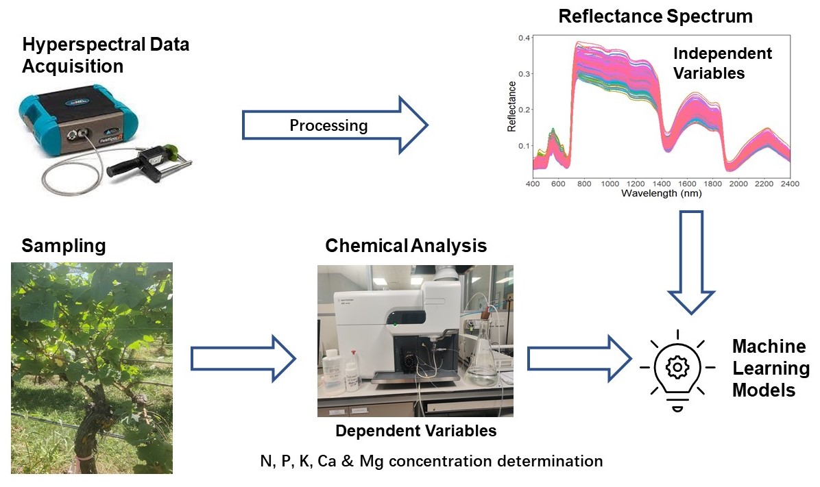
2. Methodology
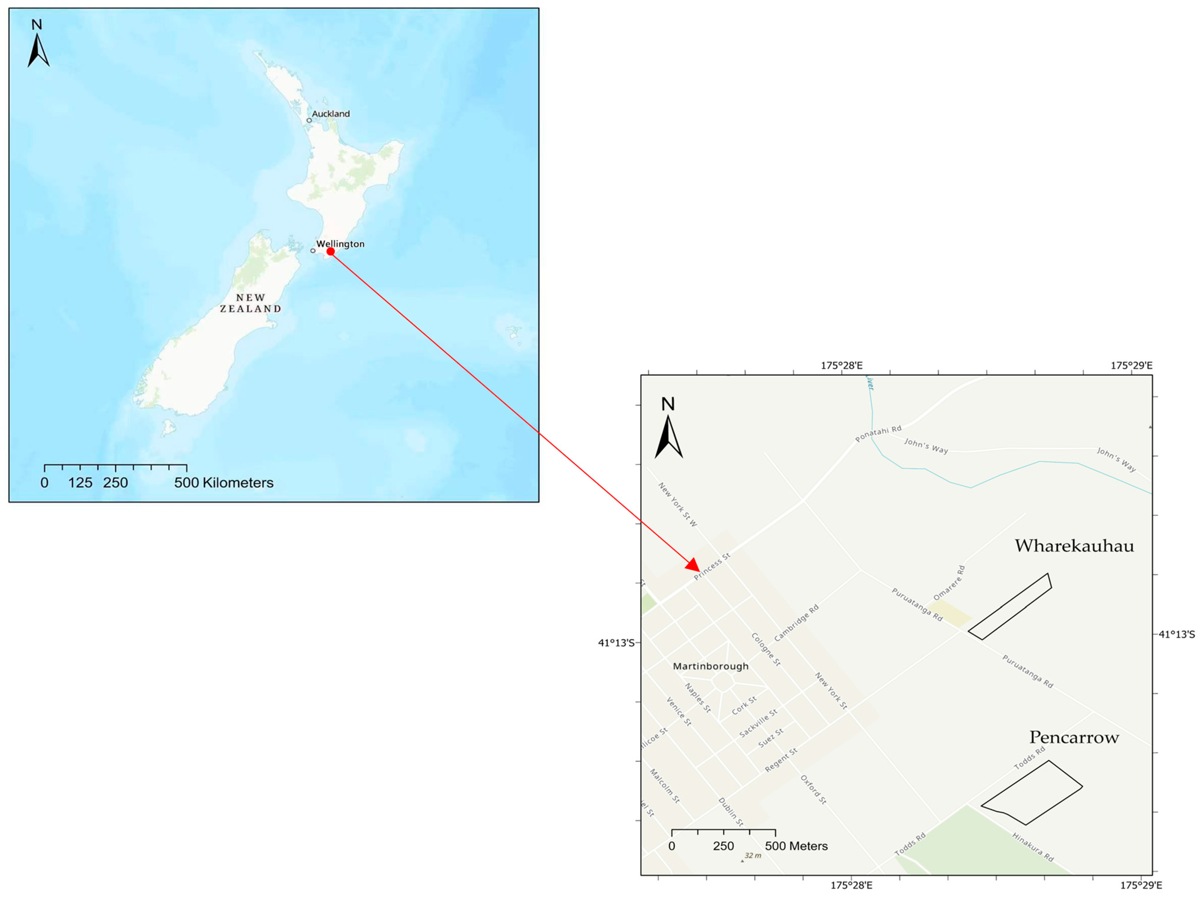
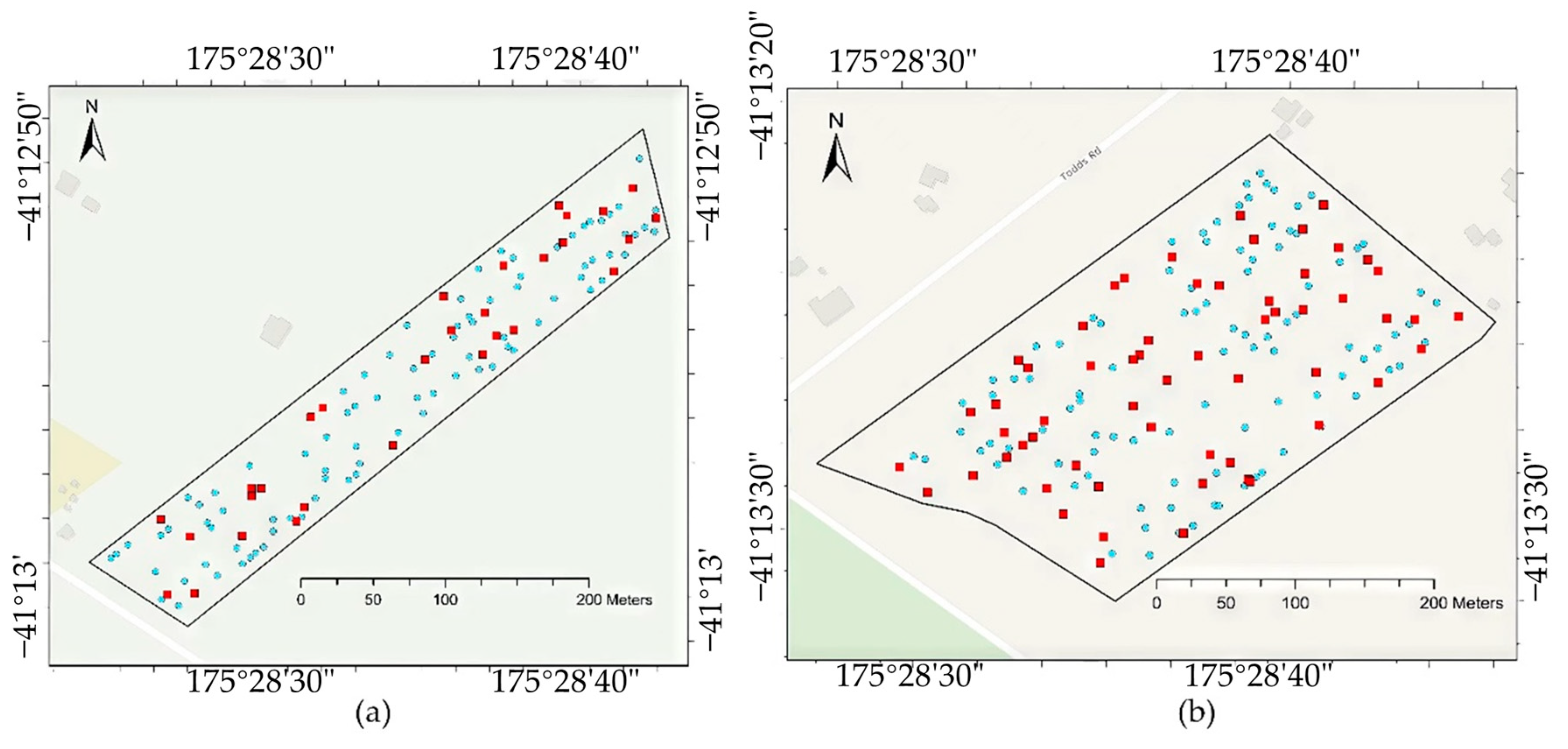
2.1. Research Sites
2.2. Sampling Plan and Chemical Analysis
2.3. Acquisition of Spectral Data
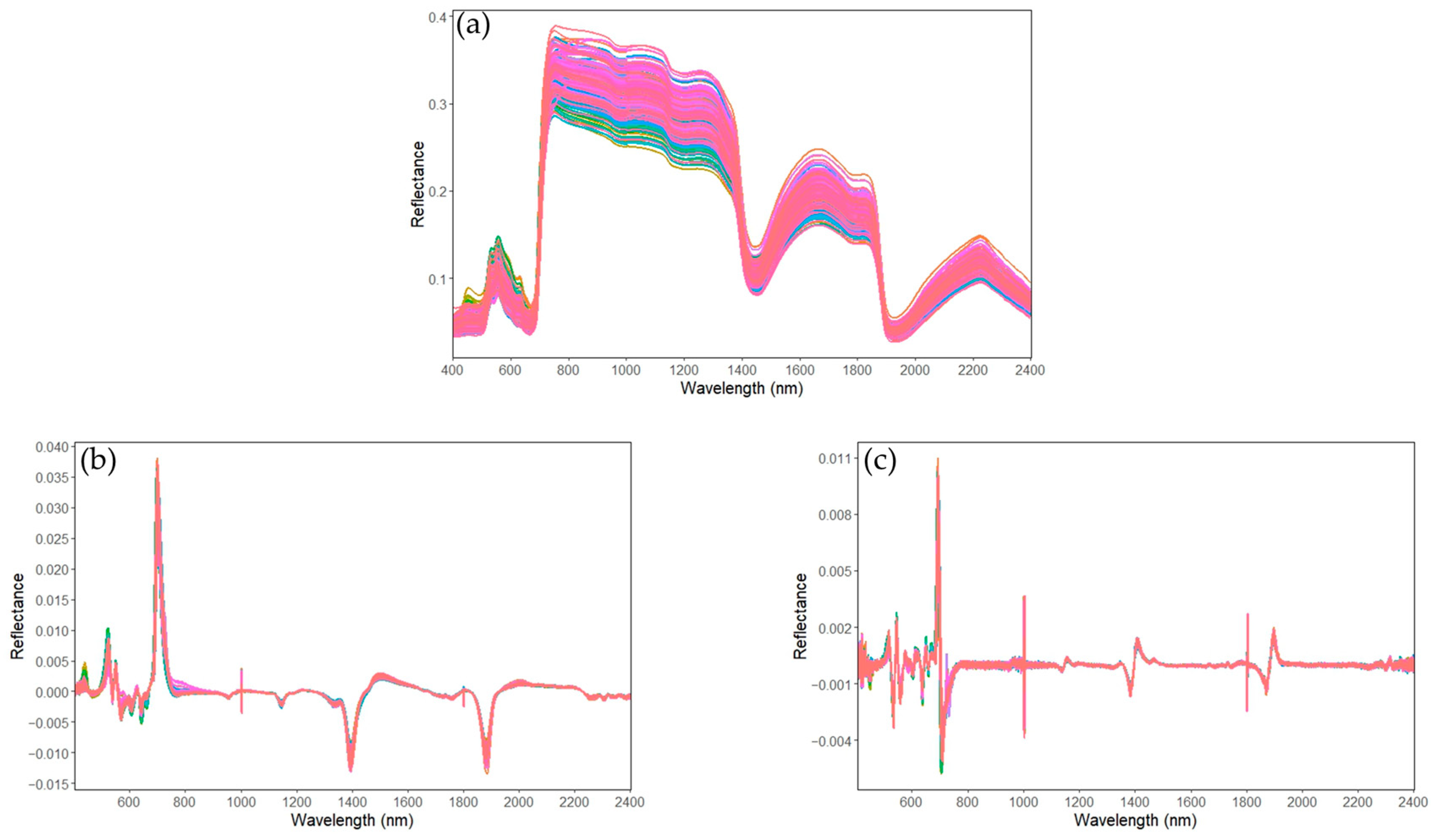
2.4. Spectral Pre-Treatments
2.5. Data Analysis

| Vegetation Indices | Acronym | Formula | Reference |
|---|---|---|---|
| Normalized difference vegetation index | NDVI | (R860 − R650)/(R860 + R650) | [36] |
| Modified Normalized Difference Vegetation Index | mNDVI | (R775 − R670)/(R775 + R670) | [37] |
| Renormalized Difference Vegetation Index | RDVI | (R800 − R670)/((R800 + R670) × 0.5 | [38] |
| Green Normalized Difference Vegetation Index | GNDVI | (R860 − R550)/(R860 + R550) | [39] |
| Chlorophyll Absorption Reflectance Index | CARI | [(R700 − R670) − 0.2 × (R700 − R550)] | [40] |
| Chlorophyll Indices | Clgreen | (R730/R530) – 1 | [41] |
| Normalized Difference Red-Edge | NDRE | (R790 − R720)/(R790 + R720) | [40] |
| Plant cell density index | PCD | R860/R650 | [42] |
| Normalized index (870, 1450) | N_870_1450 | (R870 – R1450)/(R870 + R1450) | [24] |
| Normalized index (1645, 1715) | N_1645_1715 | (R1645 – R1715)/(R1645 + R1715) | [24] |
| Modified anthocyanin reflectance index | mARI | (1/R550 − 1/R700) × R780 | [43] |
| Carotenoid reflectance index | CRI-1 | (1/R515 − 1/R565) × R790 | [43] |
| Photochemical reflectance index | PRI | (R531 − R570)/(R531 + R570) | [44] |
| Normalized difference lignin index | NDLI | (log(1/R1754)) − log(1/R1680))/(log(1/R1754) + log(1/R1680)) | [45] |
2.6. Variable Selection
2.6.1. Hierarchical Clustering
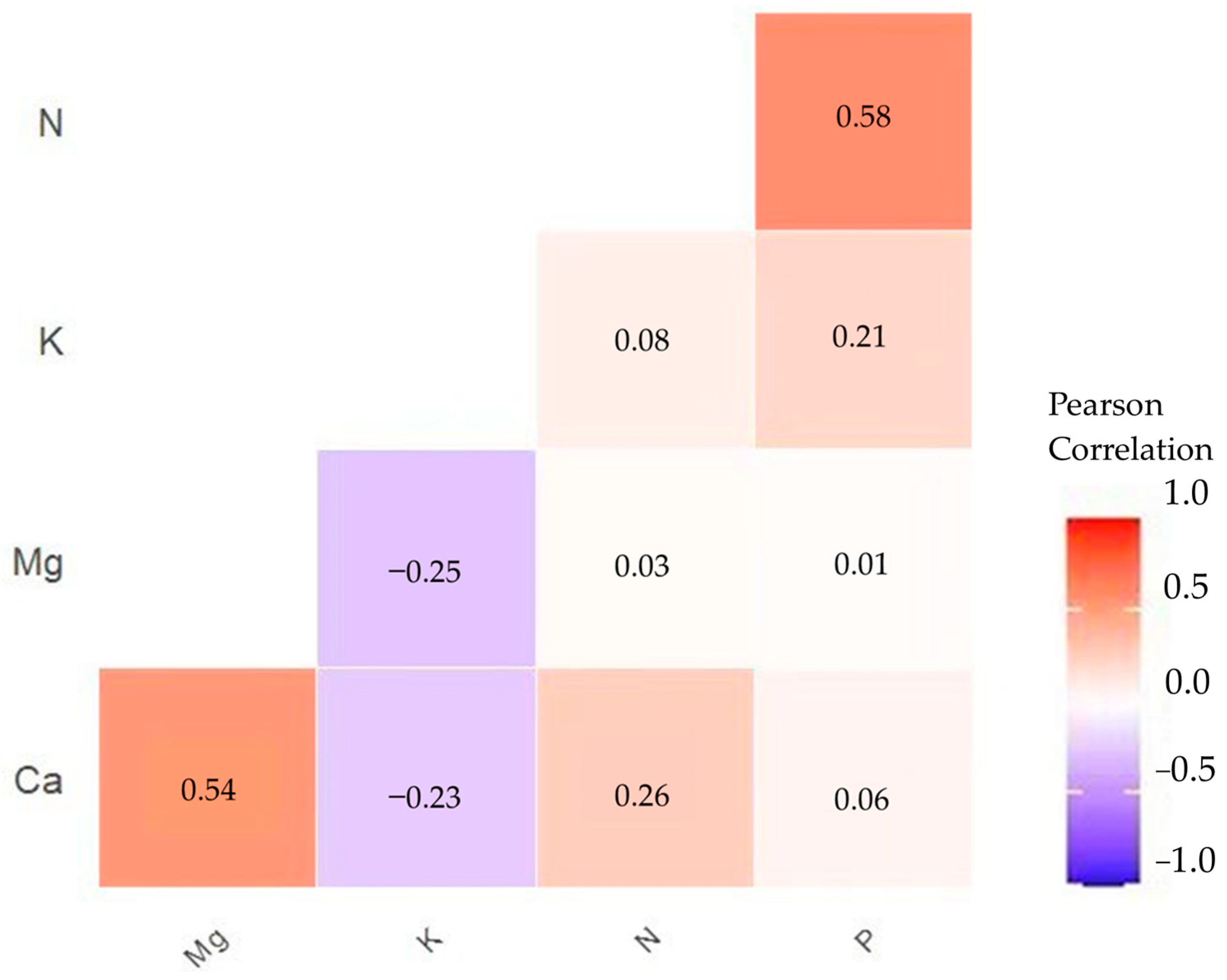
2.6.2. Pearson Correlation
2.6.3. Recursive Feature Elimination Based on Cross-Validation (RFECV)
2.7. Machine Learning Models
3. Results
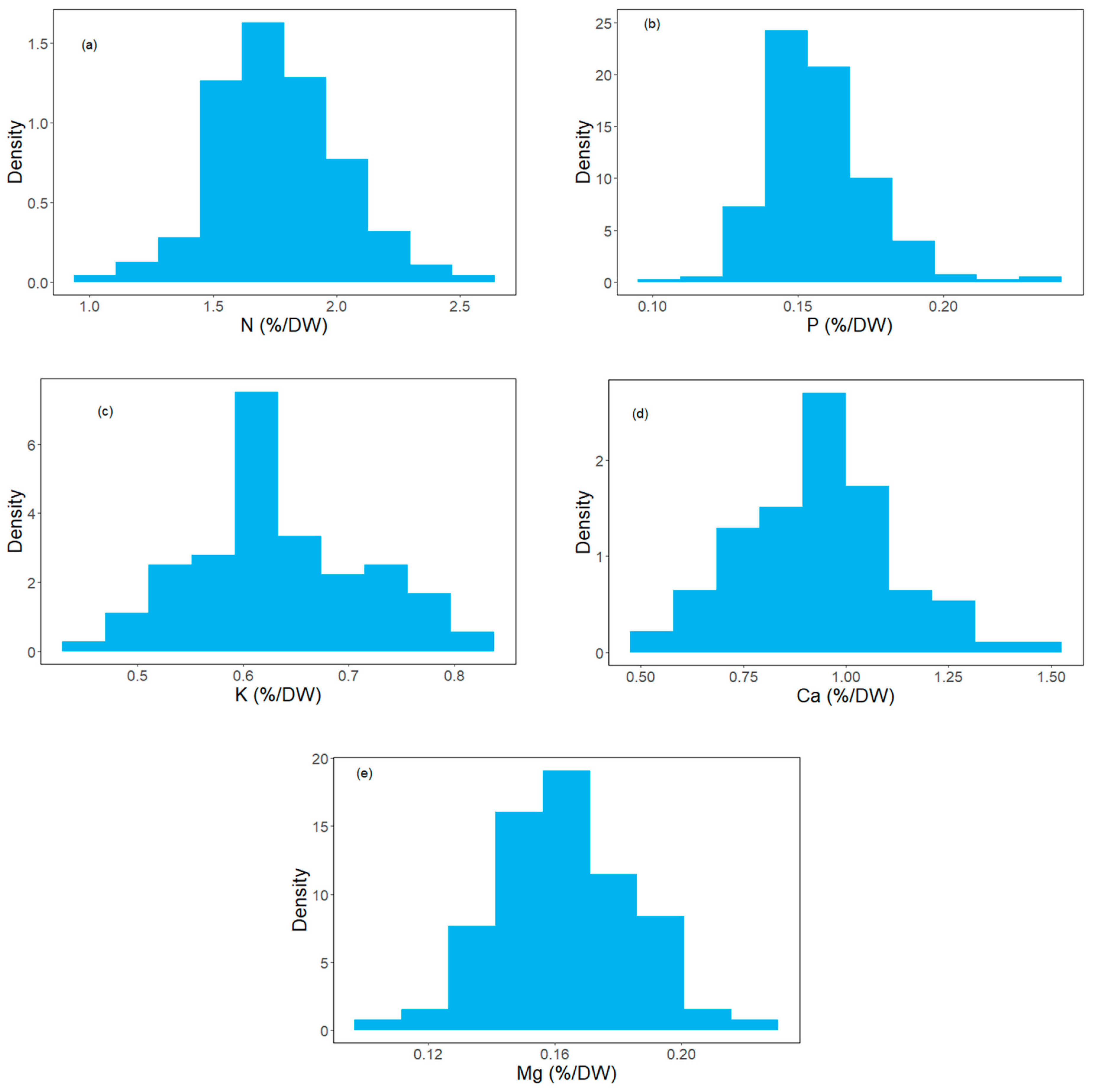
3.1. Biochemical Variables
3.2. Spectral Analysis
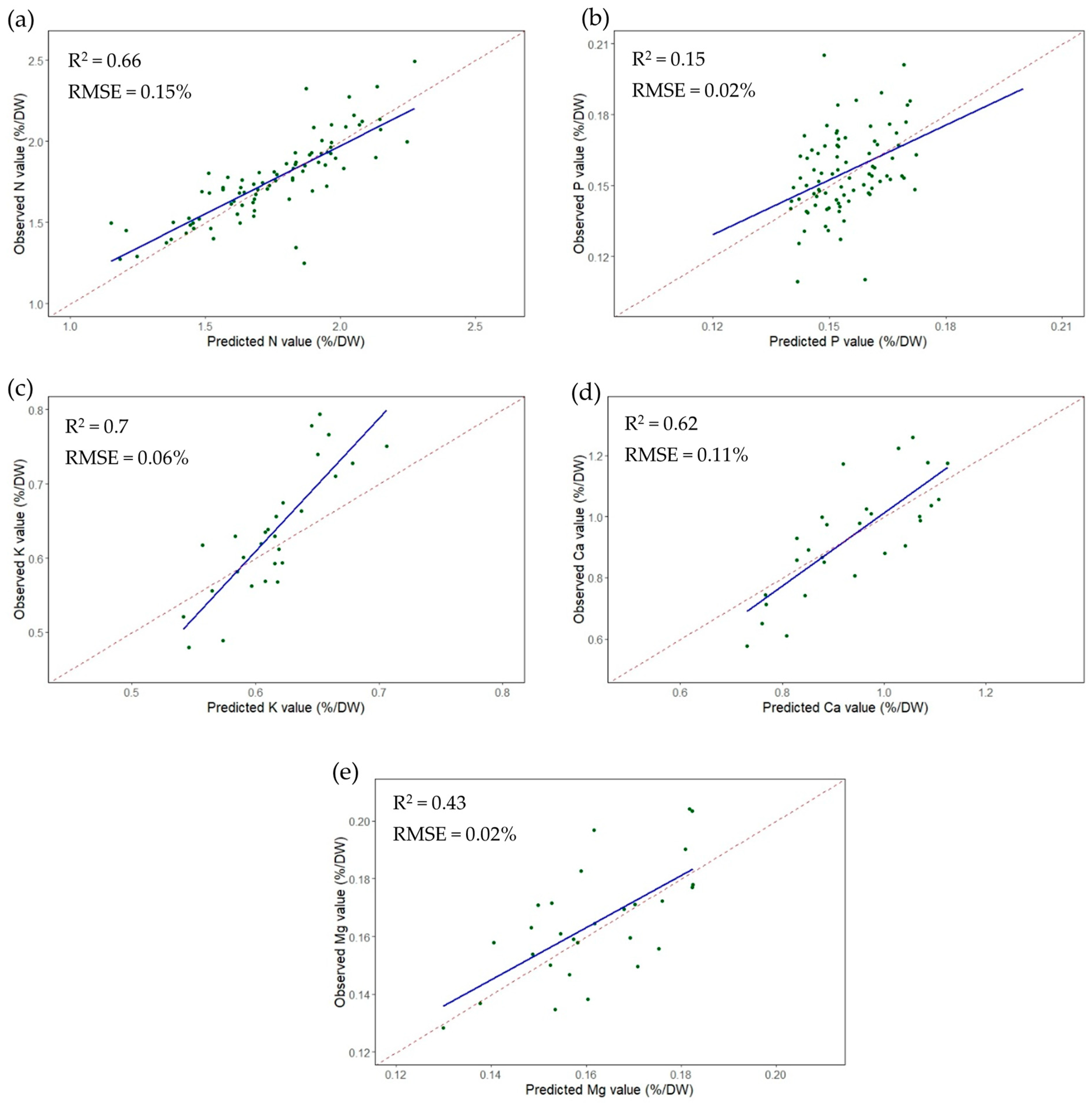
3.3. Prediction Accuracy
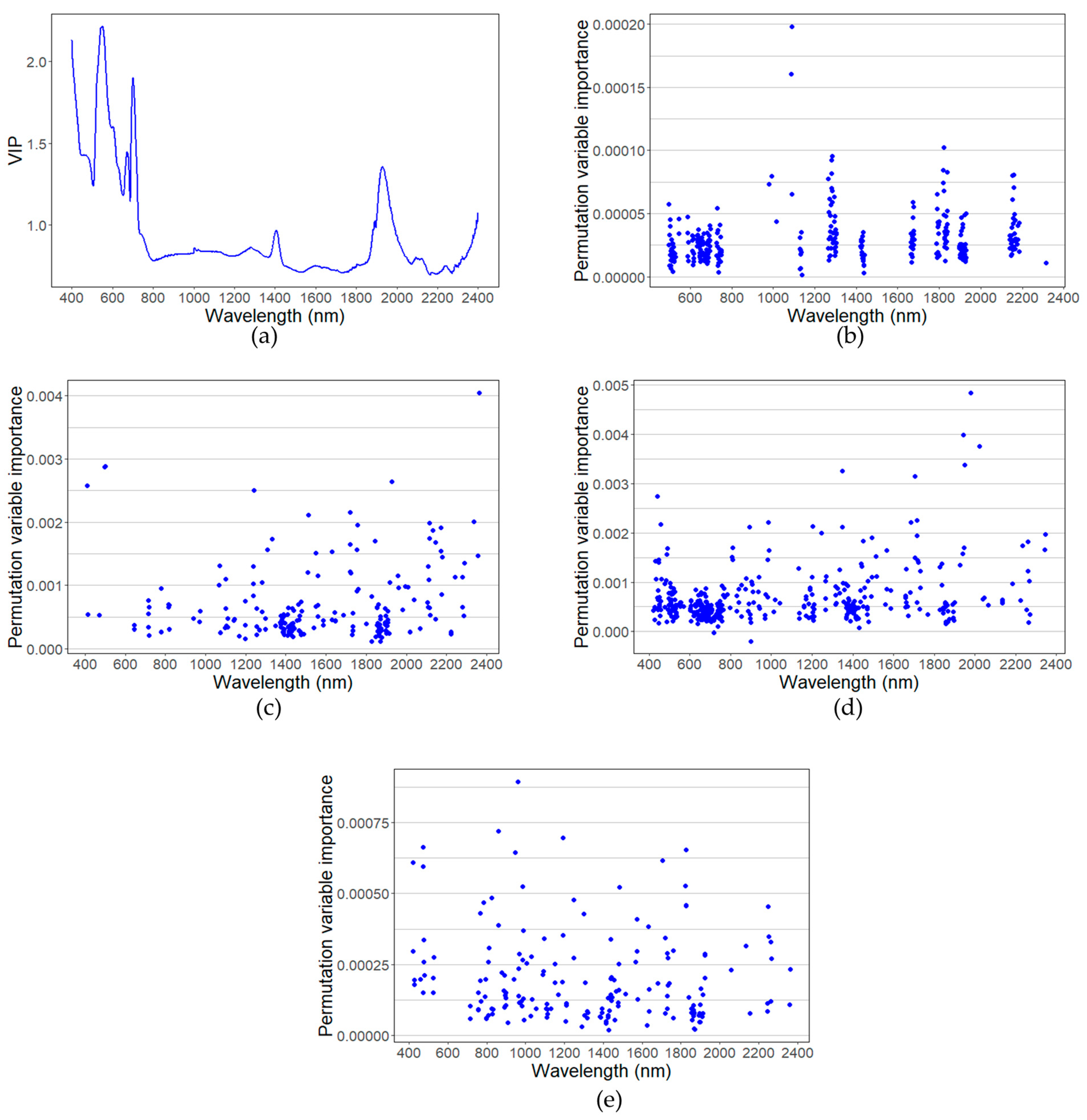
3.4. Contribution of Each Wavelength to the Algorithm
4. Discussion
5. Conclusions
Author Contributions
Funding
Data Availability Statement
Acknowledgments
Conflicts of Interest
References
- New Zealand Winegrowers. Vineyard Report 2022 New Zealand Winegrowers; New Zealand Winegrowers: Auckland, New Zealand, 2022; pp. 1–22. [Google Scholar]
- Schreiner, R.P.; Scagel, C.F.; Baham, J. Nutrient Uptake and Distribution in a Mature “Pinot Noir” Vineyard. HortScience 2006, 41, 336–345. [Google Scholar] [CrossRef]
- Chancia, R.; Bates, T.; Vanden Heuvel, J.; van Aardt, J. Assessing Grapevine Nutrient Status from Unmanned Aerial System (UAS) Hyperspectral Imagery. Remote Sens. 2021, 13, 4489. [Google Scholar] [CrossRef]
- Ashley, R. Grapevine Nutrition-an Australian Perspective; Foster’s Wine Estates Americas: Melbourne, Australia, 2011; Volume 1000. [Google Scholar]
- Debnath, S.; Paul, M.; Rahaman, D.M.; Debnath, T.; Zheng, L.; Baby, T.; Schmidtke, L.M.; Rogiers, S.Y. Identifying Individual Nutrient Deficiencies of Grapevine Leaves Using Hyperspectral Imaging. Remote Sens. 2021, 13, 3317. [Google Scholar] [CrossRef]
- Schreiner, R.P.; Osborne, J. Defining Phosphorus Requirements for Pinot Noir Grapevines. Am. J. Enol. Vitic. 2018, 69, 351–359. [Google Scholar] [CrossRef]
- Padilla, F.M.; Gallardo, M.; Peña-Fleitas, M.T.; De Souza, R.; Thompson, R.B. Proximal Optical Sensors for Nitrogen Management of Vegetable Crops: A Review. Sensors 2018, 18, 2083. [Google Scholar] [CrossRef] [PubMed]
- King, P.D.; Smart, R.E.; McClellan, D.J. Within-vineyard Variability in Vine Vegetative Growth, Yield, and Fruit and Wine Composition of Cabernet Sauvignon in Hawke’s Bay, New Zealand. Aust. J. Grape Wine Res. 2014, 20, 234–246. [Google Scholar] [CrossRef]
- Moyer, M.; Singer, S.D.; Davenport, J.R.; Hoheisel, G.-A. Vineyard Nutrient Management in Washington State; Washington State University Extension: Pullman, WA, USA, 2018. [Google Scholar]
- Schreiner, R.P. Nutrient Uptake and Distribution in Young Pinot Noir Grapevines over Two Seasons. Am. J. Enol. Vitic. 2016, 67, 436–448. [Google Scholar] [CrossRef]
- Malmir, M.; Tahmasbian, I.; Xu, Z.; Farrar, M.B.; Bai, S.H. Prediction of Macronutrients in Plant Leaves Using Chemometric Analysis and Wavelength Selection. J. Soils Sediments 2020, 20, 249–259. [Google Scholar] [CrossRef]
- Osco, L.P.; Ramos, A.P.M.; Faita Pinheiro, M.M.; Moriya, É.A.S.; Imai, N.N.; Estrabis, N.; Ianczyk, F.; Araújo, F.F.; Liesenberg, V.; Jorge, L.A.D.C. A Machine Learning Framework to Predict Nutrient Content in Valencia-Orange Leaf Hyperspectral Measurements. Remote Sens. 2020, 12, 906. [Google Scholar] [CrossRef]
- Christensen, P.; Kearney, U.C. Use of Tissue Analysis in Viticulture. In Cooperative Extension Pub. NG10-00; University of California: Visalia, CA, USA, 2005. [Google Scholar]
- Ye, X.; Abe, S.; Zhang, S. Estimation and Mapping of Nitrogen Content in Apple Trees at Leaf and Canopy Levels Using Hyperspectral Imaging. Precis. Agric. 2020, 21, 198–225. [Google Scholar] [CrossRef]
- Fu, Y.; Yang, G.; Pu, R.; Li, Z.; Li, H.; Xu, X.; Song, X.; Yang, X.; Zhao, C. An Overview of Crop Nitrogen Status Assessment Using Hyperspectral Remote Sensing: Current Status and Perspectives. Eur. J. Agron. 2021, 124, 126241. [Google Scholar] [CrossRef]
- Berger, K.; Verrelst, J.; Feret, J.-B.; Wang, Z.; Wocher, M.; Strathmann, M.; Danner, M.; Mauser, W.; Hank, T. Crop Nitrogen Monitoring: Recent Progress and Principal Developments in the Context of Imaging Spectroscopy Missions. Remote Sens. Environ. 2020, 242, 111758. [Google Scholar] [CrossRef] [PubMed]
- Bruning, B.; Liu, H.; Brien, C.; Berger, B.; Lewis, M.; Garnett, T. The Development of Hyperspectral Distribution Maps to Predict the Content and Distribution of Nitrogen and Water in Wheat (Triticum aestivum). Front. Plant Sci. 2019, 10, 1380. [Google Scholar] [CrossRef] [PubMed]
- Camino, C.; González-Dugo, V.; Hernández, P.; Sillero, J.C.; Zarco-Tejada, P.J. Improved Nitrogen Retrievals with Airborne-Derived Fluorescence and Plant Traits Quantified from VNIR-SWIR Hyperspectral Imagery in the Context of Precision Agriculture. Int. J. Appl. Earth Obs. Geoinf. 2018, 70, 105–117. [Google Scholar] [CrossRef]
- Peng, Y.; Zhang, M.; Xu, Z.; Yang, T.; Su, Y.; Zhou, T.; Wang, H.; Wang, Y.; Lin, Y. Estimation of Leaf Nutrition Status in Degraded Vegetation Based on Field Survey and Hyperspectral Data. Sci. Rep. 2020, 10, 1–12. [Google Scholar] [CrossRef]
- Oppelt, N.; Mauser, W. Hyperspectral Monitoring of Physiological Parameters of Wheat during a Vegetation Period Using AVIS Data. Int. J. Remote Sens. 2004, 25, 145–159. [Google Scholar] [CrossRef]
- Mahajan, G.R.; Sahoo, R.N.; Pandey, R.N.; Gupta, V.K.; Kumar, D. Using Hyperspectral Remote Sensing Techniques to Monitor Nitrogen, Phosphorus, Sulphur and Potassium in Wheat (Triticum aestivum L.). Precis. Agric. 2014, 15, 499–522. [Google Scholar] [CrossRef]
- Wijesingha, J.; Astor, T.; Schulze-Brüninghoff, D.; Wengert, M.; Wachendorf, M. Predicting Forage Quality of Grasslands Using UAV-Borne Imaging Spectroscopy. Remote Sens. 2020, 12, 126. [Google Scholar] [CrossRef]
- Mahajan, G.R.; Pandey, R.N.; Sahoo, R.N.; Gupta, V.K.; Datta, S.C.; Kumar, D. Monitoring Nitrogen, Phosphorus and Sulphur in Hybrid Rice (Oryza sativa L.) Using Hyperspectral Remote Sensing. Precis. Agric. 2017, 18, 736–761. [Google Scholar] [CrossRef]
- Pimstein, A.; Karnieli, A.; Bansal, S.K.; Bonfil, D.J. Exploring Remotely Sensed Technologies for Monitoring Wheat Potassium and Phosphorus Using Field Spectroscopy. Field Crops Res. 2011, 121, 125–135. [Google Scholar] [CrossRef]
- Skidmore, A.K.; Ferwerda, J.G.; Mutanga, O.; Van Wieren, S.E.; Peel, M.; Grant, R.C.; Prins, H.H.; Balcik, F.B.; Venus, V. Forage Quality of Savannas—Simultaneously Mapping Foliar Protein and Polyphenols for Trees and Grass Using Hyperspectral Imagery. Remote Sens. Environ. 2010, 114, 64–72. [Google Scholar] [CrossRef]
- Kumar, L.; Schmidt, K.; Dury, S.; Skidmore, A. Imaging Spectrometry and Vegetation Science. In Imaging Spectrometry; Springer: Berlin/Heidelberg, Germany, 2001; pp. 111–155. ISBN 978-0-306-47578-8. [Google Scholar]
- Kokaly, R.F.; Clark, R.N. Spectroscopic Determination of Leaf Biochemistry Using Band-Depth Analysis of Absorption Features and Stepwise Multiple Linear Regression. Remote Sens. Environ. 1999, 67, 267–287. [Google Scholar] [CrossRef]
- Schreiner, R.P.; Osborne, J. Potassium Requirements for Pinot Noir Grapevines. Am. J. Enol. Vitic. 2020, 71, 33–43. [Google Scholar] [CrossRef]
- Chen, L.; Lin, L.; Cai, G.; Sun, Y.; Huang, T.; Wang, K.; Deng, J. Identification of Nitrogen, Phosphorus, and Potassium Deficiencies in Rice Based on Static Scanning Technology and Hierarchical Identification Method. PloS ONE 2014, 9, e113200. [Google Scholar] [CrossRef] [PubMed]
- Mutanga, O.; Odindi, J. Exploring the Potential of Hyperspectral Data and Multivariate Techniques in Discriminating Different Fertilizer Treatments in Grasslands. J. Appl. Remote Sens. 2015, 9, 096033. [Google Scholar]
- Ponzoni, F.J.; De, J.L.; Goncalves, M. Spectral Features Associated with Nitrogen, Phosphorus, and Potassium Deficiencies in Eucalyptus saligna Seedling Leaves. Int. J. Remote Sens. 1999, 20, 2249–2264. [Google Scholar] [CrossRef]
- Yang, J.; Du, L.; Gong, W.; Shi, S.; Sun, J.; Chen, B. Analyzing the Performance of the First-Derivative Fluorescence Spectrum for Estimating Leaf Nitrogen Concentration. Opt. Express 2019, 27, 3978–3990. [Google Scholar] [CrossRef]
- Yang, J.; Cheng, Y.; Du, L.; Gong, W.; Shi, S.; Sun, J.; Chen, B. Selection of the Optimal Bands of First-Derivative Fluorescence Characteristics for Leaf Nitrogen Concentration Estimation. Appl. Opt. 2019, 58, 5720–5727. [Google Scholar] [CrossRef]
- Stevens, A.; Ramirez-Lopez, L.; Hans, G. Miscellaneous Functions for Processing and Sample Selection of Spectroscopic Data. 2022. Available online: https://cran.r-project.org/web/packages/prospectr/index.html (accessed on 5 March 2023).
- Frick, H.; Chow, F.; Kuhn, M.; Mahoney, M.; Silge, J.; Wickham, H. General Resampling Infrastructure. 2022. Available online: https://cran.r-project.org/web/packages/rsample/index.html (accessed on 5 March 2023).
- Rouse Jr, J.W.; Haas, R.H.; Deering, D.W.; Schell, J.A.; Harlan, J.C. Monitoring the Vernal Advancement and Retrogradation (Green Wave Effect) of Natural Vegetation; NTRS: Chicago, IL, USA, 1974; pp. 1–120. [Google Scholar]
- Jurgens, C. The Modified Normalized Difference Vegetation Index (MNDVI) a New Index to Determine Frost Damages in Agriculture Based on Landsat TM Data. Int. J. Remote Sens. 1997, 18, 3583–3594. [Google Scholar] [CrossRef]
- Roujean, J.-L.; Breon, F.-M. Estimating PAR Absorbed by Vegetation from Bidirectional Reflectance Measurements. Remote Sens. Environ. 1995, 51, 375–384. [Google Scholar] [CrossRef]
- Gitelson, A.A.; Merzlyak, M.N. Remote Sensing of Chlorophyll Concentration in Higher Plant Leaves. Adv. Space Res. 1998, 22, 689–692. [Google Scholar] [CrossRef]
- Sellami, M.H.; Albrizio, R.; Čolović, M.; Hamze, M.; Cantore, V.; Todorovic, M.; Piscitelli, L.; Stellacci, A.M. Selection of Hyperspectral Vegetation Indices for Monitoring Yield and Physiological Response in Sweet Maize under Different Water and Nitrogen Availability. Agronomy 2022, 12, 489. [Google Scholar] [CrossRef]
- Gitelson, A.A.; Gritz, Y.; Merzlyak, M.N. Relationships between Leaf Chlorophyll Content and Spectral Reflectance and Algorithms for Non-Destructive Chlorophyll Assessment in Higher Plant Leaves. J. Plant Physiol. 2003, 160, 271–282. [Google Scholar] [CrossRef] [PubMed]
- Arnó Satorra, J.; Martínez Casasnovas, J.A.; Ribes Dasi, M.; Rosell Polo, J.R. Precision Viticulture. Research Topics, Challenges and Opportunities in Site-Specific Vineyard Management. Span. J. Agric. Res. 2009, 7, 779–790. [Google Scholar] [CrossRef]
- Gitelson, A.A.; Keydan, G.P.; Merzlyak, M.N. Three-band Model for Noninvasive Estimation of Chlorophyll, Carotenoids, and Anthocyanin Contents in Higher Plant Leaves. Geophys. Res. Lett. 2006, 33, 6457. [Google Scholar] [CrossRef]
- Gamon, J.A.; Penuelas, J.; Field, C.B. A Narrow-Waveband Spectral Index That Tracks Diurnal Changes in Photosynthetic Efficiency. Remote Sens. Environ. 1992, 41, 35–44. [Google Scholar] [CrossRef]
- Serrano, L.; Penuelas, J.; Ustin, S.L. Remote Sensing of Nitrogen and Lignin in Mediterranean Vegetation from AVIRIS Data: Decomposing Biochemical from Structural Signals. Remote Sens. Environ. 2002, 81, 355–364. [Google Scholar] [CrossRef]
- Badr, H.; Zaitchik, B.; Dezfuli, A. Hierarchical Climate Regionalization. Authorea Preprints. 2022. Available online: https://cran.r-project.org/web/packages/HiClimR/index.html (accessed on 5 March 2023).
- Liland, K.H.; Mevik, B.H.; Wehrens, R. Paul Hiemstra Partial Least Squares and Principal Component Regression. 2022. Available online: https://cran.r-project.org/web/packages/HiClimR/index.html (accessed on 5 March 2023).
- Kuhn, M.; Wing, J.; Weston, S.; Williams, A.; Keefer, C.; Engelhardt, A.; Cooper, T.; Mayer, Z.; Kenkel, B.; Team, R.C. Classification and Regression Training. R J. 2022, 223. Available online: https://cran.r-project.org/web/packages/pls/index.html (accessed on 5 March 2023).
- Li, Z.; Jin, X.; Yang, G.; Drummond, J.; Yang, H.; Clark, B.; Li, Z.; Zhao, C. Remote Sensing of Leaf and Canopy Nitrogen Status in Winter Wheat (Triticum aestivum L.) Based on N-PROSAIL Model. Remote Sens. 2018, 10, 1463. [Google Scholar] [CrossRef]
- Lu, J.; Yang, T.; Su, X.; Qi, H.; Yao, X.; Cheng, T.; Zhu, Y.; Cao, W.; Tian, Y. Monitoring Leaf Potassium Content Using Hyperspectral Vegetation Indices in Rice Leaves. Precis. Agric. 2020, 21, 324–348. [Google Scholar] [CrossRef]
- Galvez-Sola, L.; García-Sánchez, F.; Pérez-Pérez, J.G.; Gimeno, V.; Navarro, J.M.; Moral, R.; Martínez-Nicolás, J.J.; Nieves, M. Rapid Estimation of Nutritional Elements on Citrus Leaves by near Infrared Reflectance Spectroscopy. Front. Plant Sci. 2015, 6, 571. [Google Scholar] [CrossRef] [PubMed]
- Retzlaff, R.; Molitor, D.; Behr, M.; Bossung, C.; Rock, G.; Hoffmann, L.; Evers, D.; Udelhoven, T. UAS-Based Multi-Angular Remote Sensing of the Effects of Soil Management Strategies on Grapevine. OENO One 2015, 49, 85–102. [Google Scholar] [CrossRef]
- Gil-Pérez, B.; Zarco-Tejada, P.J.; Correa-Guimaraes, A.; Relea-Gangas, E.; Navas-Gracia, L.M.; Hernández-Navarro, S.; Sanz-Requena, J.F.; Berjón, A.; Martín-Gil, J. Remote Sensing Detection of Nutrient Uptake in Vineyards Using Narrow-Band Hyperspectral Imagery. Vitis 2010, 49, 167–173. [Google Scholar]
- Wei, H.-E.; Grafton, M.; Bretherton, M.; Irwin, M.; Sandoval, E. Evaluation of Point Hyperspectral Reflectance and Multivariate Regression Models for Grapevine Water Status Estimation. Remote Sens. 2021, 13, 3198. [Google Scholar] [CrossRef]
- Wu, D.; Sun, D.-W. Advanced Applications of Hyperspectral Imaging Technology for Food Quality and Safety Analysis and Assessment: A Review—Part I: Fundamentals. Innov. Food Sci. Emerg. Technol. 2013, 19, 1–14. [Google Scholar] [CrossRef]
- Hu, N.; Li, W.; Du, C.; Zhang, Z.; Gao, Y.; Sun, Z.; Yang, L.; Yu, K.; Zhang, Y.; Wang, Z. Predicting Micronutrients of Wheat Using Hyperspectral Imaging. Food Chem. 2021, 343, 128473. [Google Scholar] [CrossRef]
- Xiaobo, Z.; Jiewen, Z.; Povey, M.J.; Holmes, M.; Hanpin, M. Variables Selection Methods in Near-Infrared Spectroscopy. Anal. Chim. Acta 2010, 667, 14–32. [Google Scholar] [CrossRef]
- Ma, L.; Liu, Y.; Zhang, X.; Ye, Y.; Yin, G.; Johnson, B.A. Deep Learning in Remote Sensing Applications: A Meta-Analysis and Review. ISPRS J. Photogramm. Remote Sens. 2019, 152, 166–177. [Google Scholar] [CrossRef]
- Axelsson, C.; Skidmore, A.K.; Schlerf, M.; Fauzi, A.; Verhoef, W. Hyperspectral Analysis of Mangrove Foliar Chemistry Using PLSR and Support Vector Regression. Int. J. Remote Sens. 2013, 34, 1724–1743. [Google Scholar] [CrossRef]
- Prado Osco, L.; Marques Ramos, A.P.; Roberto Pereira, D.; Akemi Saito Moriya, É.; Nobuhiro Imai, N.; Takashi Matsubara, E.; Estrabis, N.; de Souza, M.; Marcato Junior, J.; Gonçalves, W.N. Predicting Canopy Nitrogen Content in Citrus-Trees Using Random Forest Algorithm Associated to Spectral Vegetation Indices from UAV-Imagery. Remote Sens. 2019, 11, 2925. [Google Scholar] [CrossRef]
- Curran, P.J. Remote Sensing of Foliar Chemistry. Remote Sens. Environ. 1989, 30, 271–278. [Google Scholar] [CrossRef]
- Li, G.; Hu, Q.; Shi, Y.; Cui, K.; Nie, L.; Huang, J.; Peng, S. Low Nitrogen Application Enhances Starch-Metabolizing Enzyme Activity and Improves Accumulation and Translocation of Non-Structural Carbohydrates in Rice Stems. Front. Plant Sci. 2018, 9, 1128. [Google Scholar] [CrossRef] [PubMed]
- Tränkner, M.; Tavakol, E.; Jákli, B. Functioning of Potassium and Magnesium in Photosynthesis, Photosynthate Translocation and Photoprotection. Physiol. Plant. 2018, 163, 414–431. [Google Scholar] [CrossRef] [PubMed]
- Murphy, R.J.; Whelan, B.; Chlingaryan, A.; Sukkarieh, S. Quantifying Leaf-Scale Variations in Water Absorption in Lettuce from Hyperspectral Imagery: A Laboratory Study with Implications for Measuring Leaf Water Content in the Context of Precision Agriculture. Precis. Agric. 2019, 20, 767–787. [Google Scholar] [CrossRef]
- Solanki, T.; García Plazaola, J.I.; Robson, T.M.; Fernández Marín, B. Freezing Induces an Increase in Leaf Spectral Transmittance of Forest Understorey and Alpine Forbs. Photochem. Photobiol. Sci. 2022, 21, 997–1009. [Google Scholar] [CrossRef]


| Algorithm | Hyperparameter | Criteria |
|---|---|---|
| Patrial least squares regression | Number of components | 1:20 |
| Random forest regression | Number of trees | 250, 500, 750, 1000 |
| Number of variables to be considered for the best split | 0.05, 0.15, 0.25, 0.33, 0.4 × feature numbers | |
| Number of depths of the tree | 1, 3, 5, 10 | |
| Support vector regression | Kernel function | Radial basis kernel |
| Biochemical Variables | Minimum-Maximum | Mean ± SD | CV |
|---|---|---|---|
| N (%/DW) | 0.97–2.5 | 1.77 ± 0.25 | 14.12 |
| P (%/DW) | 0.11–0.23 | 0.16 ± 0.02 | 12.5 |
| K (%/DW) | 0.45–0.82 | 0.63 ± 0.08 | 12.7 |
| Ca (%/DW) | 0.53–1.45 | 0.94 ± 0.18 | 19.14 |
| Mg (%/DW) | 0.1–0.22 | 0.16 ± 0.02 | 12.5 |
| Method | N (n = 274) | P (n = 274) | K (n = 88) | Ca (n = 88) | Mg (n = 88) |
|---|---|---|---|---|---|
| PLSR | |||||
| R2 | 0.66 | 0.12 | 0.06 | 0.38 | 0.07 |
| RMSE | 0.15 | 0.02 | 0.1 | 0.14 | 0.02 |
| Data type | Raw reflectance | Raw reflectance | Second derivative reflectance | First derivative reflectance | First derivative reflectance |
| Variable source | Full set | Full set | Full set | Full set | Full set |
| RFR | |||||
| R2 | 0.6 | 0.13 | 0.35 | 0.51 | 0.26 |
| RMSE | 0.17 | 0.02 | 0.07 | 0.14 | 0.02 |
| Data type | Full set | First derivative reflectance | Second derivative reflectance | Second derivative reflectance | Second derivative reflectance |
| Variable source | RFECV based on hierarchical clustering | RFECV | Pearson correlation | Pearson correlation based on hierarchical clustering | Pearson correlation |
| SVR | |||||
| R2 | 0.62 | 0.15 | 0.7 | 0.62 | 0.43 |
| RMSE | 0.16 | 0.02 | 0.06 | 0.11 | 0.02 |
| Data type | Full set | First derivative reflectance | Second derivative reflectance | Second derivative reflectance | Second derivative reflectance |
| Variable source | RFECV based on hierarchical clustering | Pearson correlation | Pearson correlation | Pearson correlation | Pearson correlation |
| Linear regression | |||||
| R2 | 0.58 | 0.13 | 0.2 | 0.2 | 0.19 |
| RMSE | 0.15 | 0.02 | 0.08 | 0.14 | 0.02 |
| Variable source | CARI | NDRE | GNDVI | GNDVI | N_1645_1715 |
Disclaimer/Publisher’s Note: The statements, opinions and data contained in all publications are solely those of the individual author(s) and contributor(s) and not of MDPI and/or the editor(s). MDPI and/or the editor(s) disclaim responsibility for any injury to people or property resulting from any ideas, methods, instructions or products referred to in the content. |
© 2023 by the authors. Licensee MDPI, Basel, Switzerland. This article is an open access article distributed under the terms and conditions of the Creative Commons Attribution (CC BY) license (https://creativecommons.org/licenses/by/4.0/).
Share and Cite
Lyu, H.; Grafton, M.; Ramilan, T.; Irwin, M.; Sandoval, E. Assessing the Leaf Blade Nutrient Status of Pinot Noir Using Hyperspectral Reflectance and Machine Learning Models. Remote Sens. 2023, 15, 1497. https://doi.org/10.3390/rs15061497
Lyu H, Grafton M, Ramilan T, Irwin M, Sandoval E. Assessing the Leaf Blade Nutrient Status of Pinot Noir Using Hyperspectral Reflectance and Machine Learning Models. Remote Sensing. 2023; 15(6):1497. https://doi.org/10.3390/rs15061497
Chicago/Turabian StyleLyu, Hongyi, Miles Grafton, Thiagarajah Ramilan, Matthew Irwin, and Eduardo Sandoval. 2023. "Assessing the Leaf Blade Nutrient Status of Pinot Noir Using Hyperspectral Reflectance and Machine Learning Models" Remote Sensing 15, no. 6: 1497. https://doi.org/10.3390/rs15061497
APA StyleLyu, H., Grafton, M., Ramilan, T., Irwin, M., & Sandoval, E. (2023). Assessing the Leaf Blade Nutrient Status of Pinot Noir Using Hyperspectral Reflectance and Machine Learning Models. Remote Sensing, 15(6), 1497. https://doi.org/10.3390/rs15061497