Reconstructing 34 Years of Fire History in the Wet, Subtropical Vegetation of Hong Kong Using Landsat

Abstract

Burn-area products from remote sensing provide the backbone for research in fire ecology, management, and modelling. Landsat imagery could be used to create an accurate burn-area map time series at ecologically relevant spatial resolutions. However, the low temporal resolution of Landsat has limited its development in wet tropical and subtropical regions due to high cloud cover and rapid burn-area revegetation. Here, we describe a 34-year Landsat-based burn-area product for wet, subtropical Hong Kong. We overcame technical obstacles by adopting a new LTS fire burn-area detection pipeline that (1) Automatically uniformized Landsat scenes by weighted histogram matching; (2) Estimated pixel resemblance to burn areas based on a random forest model trained on the number of days between the fire event and the date of burn-area detection; (3) Iteratively merged features created by thresholding burn-area resemblance to generate burn-area polygons with detection dates; and (4) Estimated the burn severity of burn-area pixels using a time-series compatible approach. When validated with government fire records, we found that the LTS fire product carried a low area of omission (11%) compared with existing burn-area products, such as GABAM (49%), MCD64A1 (72%), and FireCCI51 (96%) while effectively controlling commission errors. Temporally, the LTS fire pipeline dated 76.9% of burn-area polygons within two months of the actual fire event. The product represents the first Landsat-based burn-area product in wet tropical and subtropical Asia that covers the entire time series. We believe that burn-area products generated from algorithms like LTS fire will effectively bridge the gap between remote sensing and field-based studies on wet tropical and subtropical fire ecology.

1. Introduction

Fire regimes in natural ecosystems have changed drastically over the past half century. The fragmentation of vegetation, as well as anthropogenic fire suppression, has reduced fire occurrence in some regions [1], while land clearance by fire, and the associated degradation of fire-resistant vegetation types, has increased fire frequency in other regions where natural fires were rare [2]. In recent years, the feedback between fires and climate change has attracted much attention, with fires being recognized as a significant source of carbon emissions [3,4], while changes in temperature, precipitation, and wind patterns under climate change in turn exacerbate extreme fire events [5]. Given the importance of fires as disturbance agents, both locally and globally, various aspects in the vegetation-fire feedback, including fire susceptibility [6,7], post-fire recovery trajectory [8,9], and feedback direction/strength [10], have been closely scrutinized. Understanding the influences of historical fire events on current vegetation composition and structure is essential for predicting how vegetation might respond to future fire regime shifts and managing existing landscapes in preparation for these changes.

Accurate burn-area (BA) maps are critical to research on fire regime shifts and fire-vegetation feedback. The groundwork for large-scale BA maps was laid down by products based on SPOT and ASTER optical imagery, such as L3JRC [11] and GLOBSCAR [12]. These products were largely superseded by products based on MODIS, which provided longer-running multispectral imagery with a high temporal resolution (1–2 days) [13]. In particular, MCD64A, developed by NASA [14], and FireCCI51, developed by the ESA, Ref. [15] have been widely used in recent years. MCD64A1 has mapped burn areas over a 22-year period (2000–2022) at 500 m ground resolution by detecting the thermal signature of active fires and changes in surface reflectance each day. Temporal composites were built from multiple overlapping MODIS scenes. The spatiotemporal distribution of pixels experiencing large changes in surface temperature was then used to estimate burn probabilities. The probabilities were subsequently masked and refined to daily BA maps [14]. Similarly, FireCCI51 also combines thermal anomalies and surface reflectance detected by MODIS to create daily BA maps over a similar time frame. However, FireCCI51 differs from MCD64A1 in focusing specifically on growing active fire “seeds” using the NIR band, which produces BA maps with a finer 250 m ground resolution [15].

Several studies have used MODIS-based global BA products to analyze fire patterns on global-to-regional scales [16,17,18,19], but the uptake of these products in the ecological community has been relatively slow. The commission and omission errors of existing global BA products typically exceeded 40% and 65%, respectively, with a significant discrepancy between different products [20,21,22,23,24]. For studies concerning total burn area or carbon emissions, these errors can be estimated and corrected, but for many ecological applications, these errors make it difficult for researchers to reconstruct the fire history of their areas of interest within a reasonable degree of certainty. The issue is further compounded by the low ground resolution (250–1000 m) of MODIS products, which does not relate well to field survey plots at sub-hectare spatial scales. As a result, the research on fire ecology continues to focus on single-fire events or a small handful of local fire scars, seldom combining field data with MODIS-based fire maps [25,26,27,28].

In recent years, efforts in burn-area mapping have increasingly shifted to processing imagery of higher-resolution imagery provided by the Landsat and Sentinel satellite programmes. Successive Landsat satellites have provided nearly uninterrupted global multispectral imagery at ≤30 m ground resolution since 1984 for six wavebands, namely blue, green, red, near-infrared (NIR), and two shortwave infrared (SWIR) bands. The long mission time and high spatial resolution compared to MODIS allows for the fire history of landscapes to be comprehensively reconstructed. Several regional Landsat-based fire datasets have emerged in the past few years, mostly in dry Mediterranean and temperate biomes, with burn-area maps constructed in the US [29,30], Australia [31], and Greece [32]. The high spatial resolution and accuracy of Landsat-based BA maps have enabled a large body of fire-related research [17], such as studies on fire frequency and severity trends [33,34,35,36,37,38], fire-risk modelling [39], post-fire vegetation recovery [28,40,41], and post-fire community ecology [42].

Despite these successes, there is a paucity of comprehensive Landsat-based BA maps in the wet tropics. The temporal resolution of Landsat satellites (16 days) is an order of magnitude lower than MODIS (1–2 days), making it impractical to grow burnt areas from active fires picked up by thermal bands of the Landsat sensor [43]. Thus, Landsat-based algorithms rely exclusively on changes in pixel reflectance or texture for BA detection. In some biomes, this does not greatly affect fire scar detectability. For instance, with relatively slow revegetation, BAs in temperate and arid/Mediterranean biomes are often distinguishable for years after a fire [40,43]. As such, Landsat BA mapping has become routine in these ecoregions [31,44,45,46,47,48]. In tropical savannas, grasses readily resprout, but low cloud cover means that BAs are still easily mappable across a number of post-fire Landsat scenes [49,50,51]. However, in the wet tropics/subtropics, a high cloud cover (>50%) often occludes Landsat imagery for months on end, leaving no more than a dozen of partially cloudless scenes each year [52]. Coupled with rapid revegetation that obscures burnt patches within months (Figure 3), the task eludes many existing BA mapping approaches [46]. Several studies have attempted BA mapping in the wet tropics/subtropics using Landsat imagery, but these focus on pairs of pre-selected cloudless pre-fire and post-fire scenes (Table S1). These single-scene algorithms are difficult to scale up as the effort to pre-select scenes increases markedly with the spatial and temporal breadth of the study. Additionally, in many regions of the tropics, it is not uncommon for all scenes in a year to be partially (>30%) clouded, especially for years prior to the launch of Landsat 7 in 1999 [53]. As a result, none of the single-scene studies have managed to create wet tropical BA databases at temporal scales comparable to those in temperate or Mediterranean biomes (Table S1). An alternative to the single-scene approach is to include all partially cloudless scenes and perform pairwise change detection across all unmasked pixels across every time step. Using this approach, Roteta et al. (2019) [54] successfully generated a single year (2016) BA product for Sub-Saharan Africa with Sentinel 2 data but have not, as yet, produced a time series [54]. A compromise between using single scenes and the full-time series is to create multiple seasonal or yearly composites to reduce the size of the dataset while being temporally scalable. To date, the two main studies published long-term Landsat BA products in the wet tropics, and both are based on yearly composites [38,55]. Daldegan et al. (2019) [38] created yearly medoid composites from Landsat 5/7/8 data in the Cerrado–Amazon transitionary zone in Brazil [38]. Spectral mixture analyses were then performed on the composites to separate burnt and unburnt pixels. The final product resulted in 32 yearly BA maps (1985–2017) of the study area. Long et al. (2019) [55] estimated the burnt probabilities from Landsat 5/7/8 imagery and created yearly burn-probability composites [55]. A seed-growing algorithm was then used to create a global Landsat-based BA product. At the time of writing, the dataset covers 26 years (1989, 1992, 1995, 1996, 1998, and all years between 2000 and 2020) and is freely accessible through an FTP server. Despite these current advances in Landsat BA mapping in the tropics, neither study has estimated the time of fire, but instead provided annual maps of BA locations. Approximating the fire date through the date of detection provides crucial information for evaluating the relationship between weather patterns and fire susceptibility/post-fire recovery. Additionally, ecologists are often not only interested in the extent, but also the severity of the burnt patch. Common remotely sensed indices used to estimate severity, such as dNBR, RdNBR, and RBR (reviewed in [20]), are mainly based on single pairs of pre- and post-fire Landsat scenes. The modification and incorporation of burn severity into wet tropical BA maps would be invaluable to the ecological community.

In this study, we generated a Landsat-based BA time series based on a new pipeline—LTSfire (Figure 2). Specifically, we—

(1)

Developed a preprocessing pipeline that is robust in regions affected by high cloud cover and haze.

(2)

Minimized both commission and omission errors in burn-area detection and allowed small features to be accurately detected.

(3)

Approximated the fire dates of detected burnt patches by preserving the dates of detection throughout the pipeline.

(4)

Estimated burnt severity across pixels in the detected burnt patches.

The resulting product represents the first Landsat-based BA map in wet tropical/subtropical Asia that covers the entire Landsat 5/7/8 time series. It is also the first long-term Landsat BA map in the wet tropics/subtropics that estimated both BA detection dates and burn severity.

2. Materials and Methods

2.1. Study Area

The study was conducted in Hong Kong (22°16′8″N, 113°57′6″E) over an area of 1110 km². Despite its reputation as a densely populated city, Hong Kong has an extensive countryside with over 40% of the area protected as Country Parks (Figure 1). The climate is wet subtropical, with pronounced seasons and high cloudiness (68% average cloud cover) [56]. The region was historically covered by broad-leaved evergreen rainforest, but most of the natural vegetation was deforested and degraded after centuries of human settlement and agricultural activity [57]. Under better protection following the second world war, the landscape gradually recovered into the mixture of grasslands, shrublands, and secondary forests seen today [57]. Fires are common in Hong Kong, with the Fire Services Department (FSD) reporting over 1000 outdoor fires in 2018 alone, and these fires maintain grasslands and return forests to earlier stages of succession [57]. Since natural fires are very rare under the wet subtropical climate of Hong Kong (1400–3000 mm rainfall per year), such fires are almost exclusively anthropogenic. Fire records are kept by the FSD and the Agricultural, Fisheries, and Conservation Department (AFCD), but detailed maps of fire extents have not been compiled.

2.2. Overview of the LTSfire Pipeline

The LTS fire pipeline is composed of five main sections to create BA maps with dates of detection and burn severity (Figure 2). We first collated input data, including relevant Landsat imagery and training/validation datasets (Section 2.3). Then, the Landsat scenes were preprocessed into seasonal date-traceable composites (Section 2.4). Training data were extracted from the composites to build random forest Δτ regression models (Section 2.5). The models were later used to identify potential areas that resembled BAs, which were polygonised and iteratively merged (Section 2.6). Finally, burn severity of detected BA pixels was estimated by time series-relativized burn ratio (ts-RBR) (Section 2.7).

2.3. Input Data

2.3.1. Known Burnt and Unburnt Areas

A total of 94 known burn areas dating from 1988 to 2018 were used to train a regression model and validate BA maps. The Fire Services Department (FSD) provided a list of all 2036 reported fire events of 2017 and 2018. The database included the area burnt (in m²), date the fire was reported, and the approximate location in Universal Transverse Mercator (UTM) coordinates or nearest lamp post. Most of these fires were small, so we mainly focused on features > 4000 m² (covering at least 4–5 Landsat pixels). In addition to the FSD records, we obtained a list of years and UTM coordinates for all major (>100 ha) fires between 2010 and 2017 from the Agricultural, Fisheries, and Conservation Department (AFCD). No exact fire dates were provided for this database, but the fires were significant enough so that fire dates could typically be found in local newspaper articles. Based on both the FSD and AFCD records, we manually delineated 75 burnt patches on high-resolution (<3 m) satellite images provided by Google Earth and Planet (Figure 3). When delineating the patches, we followed Stage 2 protocol outlined by the CEOS Land Product Validation (LPV) subgroup [22,59]. In particular, we checked images before and after the fire to ensure that the patch was not caused by earlier fire events. As fire dates were provided by FSD and AFCD, each polygon was associated with the exact fire data instead of temporal ranges between two images. Patches that were not clearly visible on the high-resolution satellite imagery were excluded. Since one of the aims of the pipeline is to create BA time series that spans the entire Landsat dataset, we additionally included 19 older burnt patches between 1988 and 2003 for training and validation. The UTM coordinates and fire dates of these patches were described in two local fire studies [7,60]. Neither Google Earth nor Planet data was available for these patches, so manual delineation was carried out on Landsat scenes. We recognize that CEOS LPV recommends having higher-resolution imagery when creating validation datasets, but we believe that it is still valuable to include validation data from the Landsat 5 era to test pipeline applicability across imagery collected by different Landsat sensors.

An additional 173 polygons were drawn to delineate unburnt pixels. Based on the premise that repeated burns within a year is rare, 94 of these polygons were derived from the same locations as the known burnt patches, but one season before the fire occurred. The remaining 79 polygons were urban areas and dense forests along with clouds and artifacts on the Landsat min-NBR composites. Together, these polygons cover a wide range of unburnt features, which is critical for accurate burn-area mapping [61].

2.3.2. Landsat 5, 7, 8 Surface Reflectance (SR) Scenes

Landsat 5 ETM SR, Landsat 7 ETM+ SR, and Landsat 8 OLI/TIRS SR scenes between 1986 and 2020 covering the study area were obtained through Google Earth Engine (GEE). Wavebands that were not shared between Landsat missions (e.g., the ultra-blue band in Landsat 8) were removed. The scenes already underwent basic radiometric/atmospheric correction.

2.4. Pre-Processing

2.4.1. Cloud Masking and Sorting by Season

Pixels affected by clouds in the Landsat SR scenes were masked using the cloud and cloud shadow bitmasks provided by GEE. As a fail-safe, we additionally applied a brightness threshold based on the red, green, and blue (RGB) bands to remove remaining clouds. The bands were chosen since visible light is less likely to penetrate clouds. Pixels were masked out if any one of the three bands had a reflectance > 0.2. A total of 1297 scenes with no clear pixels were removed. The remaining scenes were then sorted by season. A total of 850 summer scenes (March–October) and 685 winter scenes (November–February) from the 1986–2020 period—each covering an area of 2952 km²—were analyzed separately to maximize the probability of detecting rapidly revegetating burnt patches under pronounced seasonal effects.

2.4.2. Weighted Histogram Matching to Uniformize Landsat SR Scenes

The Landsat SR scenes were uniformized by a novel weighted histogram matching approach to minimize inter-scene differences caused by haze and changing incident sunlight (weighted histogram matching, Figure 2). We first grouped the cloudless Landsat SR scenes into five seven-year image collections (1986–1992, 1993–1999, 2000–2006, 2007–2013, 2014–2020) and created a median composite for each collection on GEE. These composites were then used as “references” to uniformize individual Landsat SR scenes. Multiple references were used to avoid uniformizing recent Landsat scenes with references from another era. We specifically chose this time interval (seven years per composites) as it provided enough cloudless scenes to create stable composites of Hong Kong while still being able to reflect decadal changes in vegetation structure. Since Hong Kong has a high cloud cover (68%) [56] and has recently experienced relatively drastic changes in vegetation structure [62], we believe that the seven-year benchmark should generally be robust enough for other wet tropical or subtropical regions. Each Landsat SR scene was paired with two reference composites according to the date of capture. For instance, a scene taken on 24 July 2013 was paired with the 2007–2013 and 2014–2020 summer reference composites. We then performed histogram matching using the histMatch function in the RStoolbox package (version 0.2.6) [63] in R-4.1.0 [64] to match each scene with the two paired references to create two matched rasters. The histMatch function compares the distributions of pixel brightness (histograms) of the source raster with the reference. It then makes adjustments to the brightness of the source raster such that the histogram matches that of the reference. The six bands were matched separately to correct systematic differences in reflectance ratios between different bands. Since urban areas and water bodies were often highly variable from scene to scene, non-vegetated pixels were masked out before matching. A weighted average was then taken between the two histogram-matched rasters based on time difference between the scene and the median date of the two references. This created a uniformized Landsat SR scene that was more inter-comparable with other uniformized scenes. Weighted histogram matching was repeated across all scenes to create 1535 uniformized Landsat SR scenes (865 summer and 685 winter).

2.4.3. Date-Traceable Compositing (Using Min-NBR as Criterion)

The uniformized Landsat SR scenes were distilled into 35 summer and 35 winter composites over the 35-year study period by date-traceable min-NBR compositing (date-traceable compositing, Figure 1). We generated seasonal composites to increase the signal-to-noise ratio and reduce data volume by selecting the pixel in the season that most resembles burn areas. We used minimum normalized burn ratio (min-NBR), based on the NIR (0.77–0.9 μm) and SWIR2 (2.08–2.35 μm) bands, as the compositing criterion. The index is chosen for its ability to identify pixels that resemble burnt patches [20].

For each pixel, we identified the scene in the season with the lowest NBR. We then transferred the reflectance of the six Landsat bands to the seasonal composite. We kept the date of capture and stored it as an extra seventh band. This allowed us to build regression models on burnt-area age using our training dataset and predict fire dates within seasonal composites in later stages of the pipeline (Section 2.5 and Section 2.6 in Figure 2).

2.4.4. Vegetation Indices (VIs), Normalization, and Inter-Annual Changes

Several additional steps were taken to preprocess the seasonal composites to suppress both commission and omission errors in BA detection. Seven vegetation indices (VIs), namely the Burned Area Index (BAI), Mid-Infrared Burn Index (MIRBI), Normalized Burn Ratio (NBR), Enhanced Vegetation Index (EVI), Normalized Difference Vegetation Index (NDVI), Simple Ratio (SR), and Soil Adjusted Vegetation Index (SAVI) were added to the seasonal composites. These VIs utilize NIR and/or SWIR bands to highlight fire-affected regions (Figure 3) and have been shown to improve separability of burnt patches in the wet tropics [65]. Additionally, the six Landsat wavebands were normalized by dividing them with the average reflectance of the same pixel as suggested by Wu (2004) and Chan et al. (2021) [66,67]. Finally, a distinctive feature of burn areas is the sudden change in spectral features from pre-fire vegetation and post-fire patches [13,68]. Hence, in addition to current-year data, inter-annual changes were calculated by subtracting the reflectance and VIs of the previous year from that of the current year.

2.5. Model Building

We built random forest (RF) regression models to detect burn area from remotely sensed data (model building, Figure 2). The RF regression models were built using the randomForest package (version 4.6–14) [69] in R-4.1.0 [64] with ntree = 500 and mtry = 5. The explanatory variables of the models were normalized reflectance, VIs, and associated interannual changes. The response variable was the estimated number of days since the last fire (Δτ), ranging from 0 to 365 days. The model took the form:

Days since fire (Δτ) ~ reflectances (6 bands) + VIs (7 indices) + changes (6 bands, 7 VIs)

We chose the number of days between the date of detection and the known fire date (Δτ) as the response variable, since it carries more information than a simple binary fire/non-fire variable: the long return time of Landsat and high cloud cover means that many known burnt areas were only detected from space months after the fire event, by which time they were partially revegetated. Δτ served as a useful proxy for pixel resemblance to burnt areas. A smaller Δτ indicated higher pixel resemblance to burnt areas, while a larger Δτ indicated resemblance to fully revegetated or unburnt pixels. For pixels in the 94 known burn areas, we calculated Δτ and extracted the 26 explanatory variables from the date-traceable Landsat composites. For pixels in the 173 unburnt polygons, we extracted the 26 explanatory variables and assigned pixels with a Δτ of 365 days, which is the largest value of Δτ a known BA pixel could take (i.e., a fire broke out in the first day of a season but was only detected in the last day of the next season) and an interval long enough for optical properties of BAs to recover (Figure 3).

To estimate the accuracy of the LTS fire product the extracted data were randomly split into 10 folds for cross validation. Since there were way more unburnt than burnt pixels, we performed stratified random sampling in each fold to ensure that the ratio between unburnt and burnt pixels was capped at 1.5. This prevented extreme class imbalances from biasing the model predictions [70]. In each of the 10 iterations, 9 out of the 10 folds were used to train an RF model. The remaining fold was kept unseen throughout the pipeline and was only used to validate the final burn-area map produced after shaping burn-area polygons (burn-area shaping, Figure 2). When creating the 10-folds, pixels extracted from the same polygon were always grouped into the same fold. This ensured that the cross-validation was always carried out across sites. In other words, if pixels from a BA polygon were used to build the fire map, we would avoid using other pixels from the same polygon to validate the results. We trained 10 RF models from the 10-folds, which were passed onto the next stage of the pipeline. Finally, to assess whether the preprocessing pipeline improved accuracies in burn-area detection, we repeated the 10-fold cross validation exercise and trained RF models using non-uniformized/normalized Landsat SR bands and VIs as inputs (referred as no-preprocessing, or NPP below).

2.6. Burn Area Shaping

2.6.1. Applying Models to Landsat Time Series and Thresholding Δτ Rasters

The RF models were then used to predict Δτ from the time series of seasonal LS composites. Each model generated a seasonal time series of 68 Δτ rasters with pixel values ranging from 0 to 365 (Figure 4).

Burnt and unburnt pixels were not easily separable by a single threshold on Δτ, so burn-area polygons were created by twice thresholding the Δτ rasters followed by seed-growing (thresholding, Figure 2). As shown in Figure 4, some unburnt pixels often had lower Δτ than some of the less severely burnt pixels in BAs. Using a single threshold would either omit a substantial number of BA pixels or mistake many unburnt pixels as burnt (Figure 5). Hence, a two-phase region-growing algorithm, similar to that described in Bastarrika et al. (2011), was adopted [45]. In the first phase, two thresholdswere applied—one stringent and one lenient—on the estimated Δτ rasters. This created two sets of polygons: the seed polygons minimized commission errors by keeping only the most severely burnt pixels (red, Figure 5); the growth polygons minimized omission errors by including pixels that resembled burnt patches (blue, Figure 5). In the second phase, we removed small-seed polygons (less than three pixels in size), which often represented artifacts [55], then overlaid the two sets of polygons and grew the seeds with intersecting growth polygons. Since most burnt patches would at least contain a few severely burnt-seed polygons that unburnt patches were unlikely to possess, and less severely burnt pixels would be captured by the growth polygons, the algorithm boosts both specificity and sensitivity in BA detection [45]. The two thresholds adopted in this study were derived from the training datasets. For each iteration in the 10-fold cross validation, we performed a smaller nine-fold cross validation within the training dataset, creating nine RF models that estimated Δτ from the holdout. We then applied thresholds ranging from 0 days to 365 days on the estimated Δτ and plotted the error-threshold curves for (1) pixel-omission error, (2) patch-omission error, and (3) pixel-commission error (Figure 5). The stringent threshold was set after the sharp drop in site-omission errors, while the lenient threshold was set after the drop in pixel-omission errors. We observed that the error-threshold curves were similar across different folds, so for simplicity, we set a single set of stringent (70 days for summer; 60 days for winter) and lenient (160 days) thresholds across all 10 folds (Figure 5). Thresholds were chosen by qualitative assessment of the error-threshold curves in this study, but these thresholds could potentially be derived mathematically in the future.

2.6.2. Iterative Polygon Merging

BA polygons over the 34-year study period were iteratively merged to create a single shapefile with a single dated polygon per BA. Despite quick vegetative recovery in the wet tropics/subtropics, it is not uncommon for the same burnt patch to be detected across multiple seasons, with complex overlapping of polygons. To prevent repeated observations from erroneously inflated estimated burn area, polygons needed to be appropriately dated and merged. Figure 6 shows the decision tree used to handle seed and growth polygons based on two criteria: seed detection date (T) and seed area (A). We used attributes from seed polygons rather than growth polygons as merging criteria, since seed polygons represent areas with high confidence in detection and were less affected by artifacts. The seed-detection date (T) was calculated by taking the earliest date of detection amongst encapsulated pixels; the seed area (A) was the area of the entire seed polygon (Figure 6). For each growth polygon, we first checked whether it contained seed polygons from the same season. If it did not, we checked whether it intersected with polygons from the previous season. Growth polygons that do not intersect with seed polygons of the same season or merged polygons from last season were discarded (rightmost branch, Figure 6). Growth polygons that only intersected with merged polygons from last season often represented genuine burnt patches, though many were not fully detected last season due to cloud occlusion or gaps between Landsat 7 scan lines. Hence, we merged these polygons together and adopted the seed date and seed area of polygons from last season (second branch from the right, Figure 6). For growth polygons that contained seed polygons from the same season, we first merged the growth polygons with the seed polygons. The resulting polygon took the date and area from the seed polygon. If the growth polygon contained more than one seed polygons, we took the date from the largest seed polygon and the area by summing areas of all intersecting seed polygons (black box after first split, Figure 6). We then checked whether the polygon overlaps with polygons from last season. If it did not, the feature likely resulted from a new fire this season, so we kept it as a separate polygon (third branch from the left, Figure 6). If it did, the polygon either resulted from two fires at close proximity or was part of a burnt patch from last season. We did not have enough information to separate the two scenarios, so we opted for an area-based approach to ensure that the dates of large patches would not be unduly dragged behind by small fires or artifacts. If the polygon from this season carried a significantly (>50%) larger seed area, we merged the polygons and adopted the new seed date and area (leftmost branch, Figure 6). Otherwise, we still merged the polygons but adopted the date from the largest overlapping polygon from the last season and the seed area from all overlapping polygons from last season (second branch from the left, Figure 6). Once all polygons from a particular season were sorted and merged following the criteria set out by Figure 6, we moved on to the next season. By iteratively adding polygons from all 68 seasons, we condensed all features into a single vector layer with overlapping features ± 1 season apart merged, and fire date estimated for each feature. In our validation exercise, iterative polygon merging was repeated 10 times for both the preprocessed and no-preprocessing datasets, creating 20 LTS fire maps. All steps were carried out in R-4.1.0 with polygons merged using the sf package (version 1.0–1) [64,71].

2.7. Burn Severity Estimation

The burn severity of pixels in the burn-area polygons were estimated by a modified version of Relativized Burn Ratio (RBR) described in Parks et al. (2014) [72] (Burn severity estimation, Figure 2). The existing RBR described by Parks et al. (2014) [72] is calculated in three steps based on a pair of Landsat scenes captured before and after the fire.

NBR = (NIR − SWIR2)/(NIR + SWIR2)

(1)

dNBR = (NBR_prefire − NBR_postfire) × 1000 − dNBR_offset

(2)

RBR = dNBR/(NBR_prefire + 1.001)

(3)

The dNBR_offset term represents the change in NBR unrelated to fire and is usually estimated from pixels outside the burn area. Other terms are self-explanatory. In this study, we kept the general structure of the equations but replaced the terms in (2) and (3) to create the time series Relative Burn Ratio (ts-RBR), a new variant of RBR derived from multiple, instead of single, pre- and post-fire scenes. This is critical in our wet subtropical study area as cloudless scenes capturing the entire landscape pre- and post-fires were often unavailable. An approach that calculates burn severity by combining information from multiple overlapping scenes is, therefore, needed.

ts-dNBR = (NBR_{med prefire} − NBR_min postfire) × 1000 − dNBR_{med min offset}

(4)

ts-RBR = ts-dNBR/(NBR_{med prefire} + 1.001)

(5)

For pre-fire conditions, we replaced the NBR_prefire term with the median pre-fire NBR (NBR_{med prefire}) calculated across all uniformized Landsat scenes (Section 2.4, Figure 2) in the season before the fire. We then replaced the NBR_postfire term with the minimum NBR (NBR_{min prefire}) across all uniformized Landsat scenes in the two seasons after the date of detection. The minimum was taken to prioritize the pixels showing the highest burn severity over those recorded after the patch starts to revegetate. An issue with differencing NBR_{med prefire} and NBR_{min postfire} is that the pre-fire median is expected to be larger than the post-fire minimum, resulting in overestimated burn severity. This was accounted for by adjusting the dNBR_offset term, which now represents the mean difference between NBR_median and NBR_minimum amongst unburnt pixels. Different dNBR_offset values were used for the three vegetation types (grasslands, shrublands, forests) based on a Landsat-based vegetation map time series of the area (unpublished). A comparison was made between the ts-RBR across grasslands, shrublands, and forests to assess whether the approach properly relativized burn severity across various vegetation types. We did not conduct field surveys to validate the burn severity estimated by ts-RBR, but mathematically, ts-RBR is near-equivalent to RBR and is expected to perform similarly as RBR.

2.8. Comparison with Other Burn Area Products

The accuracy of the LTS fire map and three global BA products (MCD64A1 version 6, FireCCI51, and GABAM) were assessed by comparing detected BAs with known fire/non-fire polygons (see Section 2.3). We polygonised and downloaded all three datasets from Google Earth Engine and the GABAM FTP server. The attributes of polygon contained estimated fire date (for MCD64A1 and FireCCI51) or year (GABAM). We overlaid the detected BA polygons onto the known fire/non-fire polygons delineated based on government fire records (Section 2.3) and analyzed the degree of overlap. For LTS fire, since all the known fire/non-fire polygons were used to train the final product, we instead carried out 10-fold cross-validation using LTS fire maps built from different subsets of the training data (see Section 2.5). In other words, we overlaid the set of validation polygons on the version of the LTS fire map built from an RF model that was not trained by pixels in the validation polygons. Since estimated fire dates were not always accurate, especially for the temporally coarse GABAM dataset, we matched features that were ± 1 year apart. We then calculated site omission (proportion of known BA polygons completely omitted), area omission (proportion of burnt area omitted), area commission (proportion of unburnt area mistaken as burnt patches), and overall accuracy (proportion of correctly classified area) from the confusion matrix. Additionally, we investigated into how accurately the iterative polygon merging algorithm dated the LTS fire polygons by plotting a histogram showing the difference between LTS fire estimated date of detection and actual fire date.

Apart from comparing burn-area products with a small number of manually delineated fire/non-fire polygons, we also evaluated the LTS fire dataset through a full intercomparison with established global burn-area products. We followed the protocol of matching features dated ± 1 year from each other. For GABAM, no fire dates were estimated, so we dated the features to the middle of the year and matched LTSfire features dated ± 365 days from the 1st of July. Additionally, at the time of writing, GABAM only included several scattered years before 2000, making it difficult to accurately match features with LTS fire. Hence, we focused our comparison on years after 2001. For each pairwise comparison between LTS fire and existing burn-area maps, we tallied the number of overlapping and non-overlapping features to obtain feature agreement. We also calculated the overlapping and non-overlapping area to get area agreement.

Finally, we used videos, figures, and graphs derived from the LTS fire map to visualize the seasonal-to-decadal trends in fire occurrence across Hong Kong. We created a time-lapse video that plots LTS fire polygons against yearly Landsat median composites at the estimated date of detection. The Temporal Controller functionality in QGIS 3.18 [73] was used to date vector and raster datasets, with the output converted to .mp4 format with FFmpeg [74]. The LTS fire map was also used to provide a holistic overview of the fire regime of the study area. We investigated the change in burn area between 1987 and 2020, analyzed seasonal fire prevalence, and tallied the number of times each pixel burnt throughout the study period.

3. Results

3.1. Validation with Known Burnt Patches

LTS fire with the full pre-processing pipeline had the highest overall accuracy and lowest omission errors amongst the burn-area products compared (

Table 1. Accuracies of LTS fire and existing global burn-area products. The burn-area maps were compared with 94 known burn-area polygons and 173 unburnt polygons. Site omission errors refer to the proportion of undetected burn-area polygons (no overlap at all); area omission errors refer to the proportion of burnt area omitted; commission errors refer to the proportion of unburnt area misclassified as burnt; and the overall accuracy refers to the overall proportion of correctly classified area. Numbers representing the highest accuracy or lowest error is bolded.

Dataset	Overall Accuracy	Site Omission Error	Area Omission Error	Commission Error
LTSfire	0.952	0.0319	0.112	0.0242
LTSfire no pre-processing	0.935	0.0851	0.175	0.025
GABAM	0.860	0.565	0.493	0.012
FireCCI51	0.720	0.987	0.960	0
MCD64A1	0.799	0.949	0.720	0

). The full LTS fire map detected 96.8% of all validation burn-area polygons and 88.8% of the known burnt area. The Landsat sensor type does not seem to significantly affect burn-area detection. Lower-area omission errors were observed before the launch of Landsat 8 in 2013 (5.6%) or before the launch of Landsat 6 in 1999 (6.3%). The algorithm misclassified 2.42% of the unburnt pixels. It is important to note that out of the 173 non-fire polygons, 94 were created by encircling pixels a few months before fires broke out (pre-fire). These polygons could easily be misclassified if the fire events were misdated during iterative polygon merging. If these polygons were excluded, errors of commission were very low (0.5% by area). If we adopted a less rigorous preprocessing pipeline and skipped weighted histogram matching (no pre-processing, Section 2.4), commission errors slightly increased and omission errors approximately doubled (Table 1). GABAM, a Landsat-based global burn-area product, detected 43.5% of the known burnt patches, or 50.7% of the burnt area in the validation dataset. A higher site omission than area omission indicates that the dataset disproportionally omitted smaller patches. The errors of commission were low overall (1.2% by area) but higher than the two LTS fire datasets if we excluded pre-fire polygons prone to misdating (1.18%). The two MODIS-based burn-area products generally had very high omission errors (Table 1), likely due to the low spatial resolution of the source data, while commission errors were negligible (0%) for both datasets.

The date of BA detection derived from iterative polygon merging was moderately successful in estimating the actual fire date. Some 62.6% of the estimated date of BA detection was within one month (±30 days) of the actual fire date, and some 76.9% of the dates were within two months (±61 days) of the actual fire event (Figure 7). Given the low (16-day) temporal resolution of the input Landsat data, the dates of BA detection were usually later than the actual fire date. However, a small number of BA polygons were misdated to dates earlier than the actual fire, possibly due to erroneously adopting the wrong date of detection from nearby fires or artifacts (Figure 7).

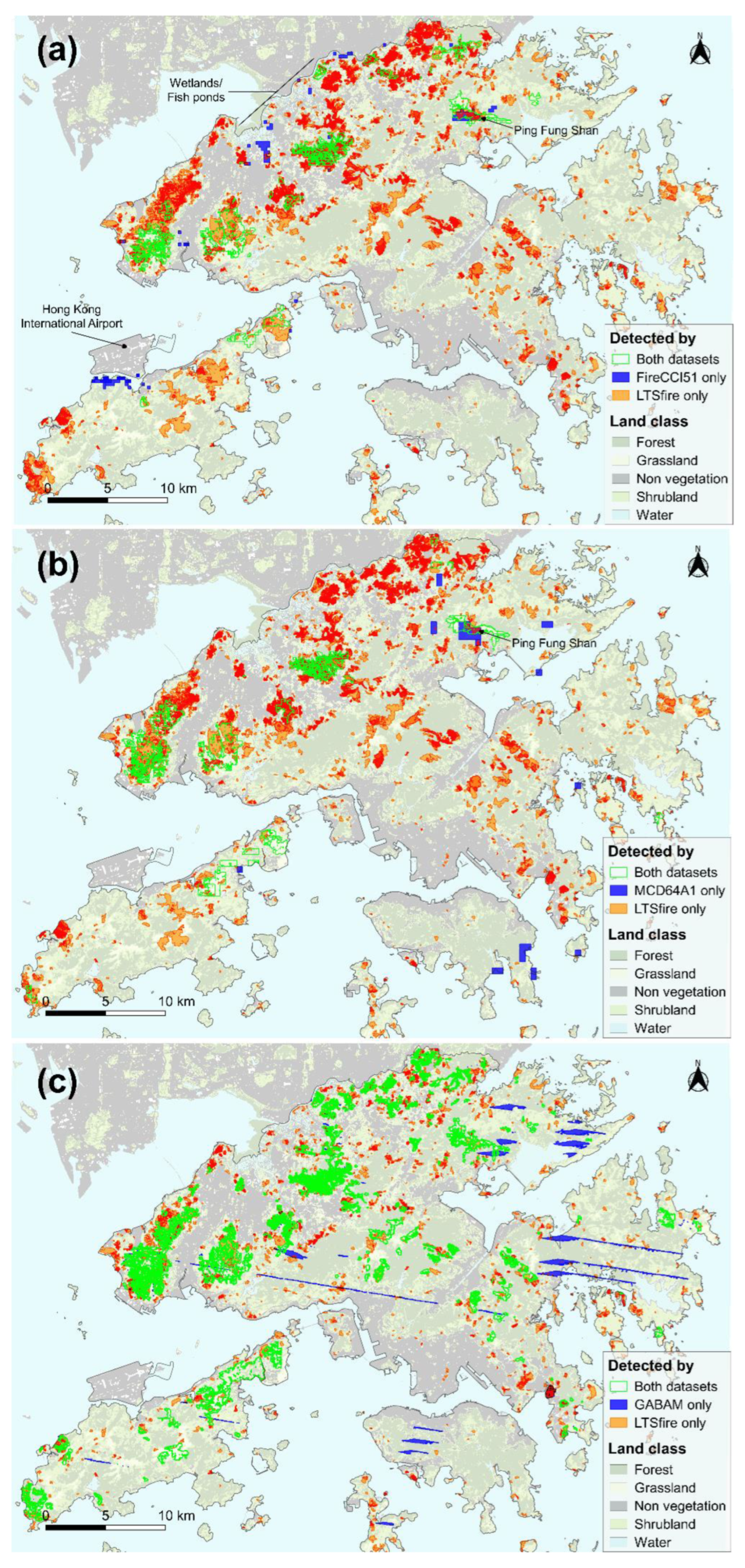
3.2. Evaluating the LTSfire Map against the MCD64A1, FireCCI51, and GABAM

Comparisons with existing burn-area products highlighted the ability of LTS fire in accurately identifying smaller BA features. MODIS-based MCD64A1 and FireCCI51 only detected 3% and 3.6% of LTSfire features, respectively (Figure S1). The datasets did manage to detect several of the largest fires (Figure 8a,b), but even by area, the omitted patches accounted for >80% of the total burnt area detected by LTS fire (Figure S1). In comparison, LTS fire detected a majority of features in both MCD64A1 (73.1%) and FireCCI51 (57.7%), and most features undetected by LTSfire were not fires but artifacts associated with the airport, urban fringes, and fishponds (Figure 8a,b). A relatively higher agreement was observed between LTS fire and GABAM. The two datasets agreed on 40.7% of the burnt patches and had a Sørensen–Dice coefficient of 0.521 (Figure S1). However, the dataset, still omitted most of the smaller local fires (Figure 8c). Several large Landsat 7 scan lines were mistaken as burnt patches in GABAM (Figure 8c), while LTSfire commission errors were mainly smaller features at fringes of urban areas and water bodies (Figure 8c).

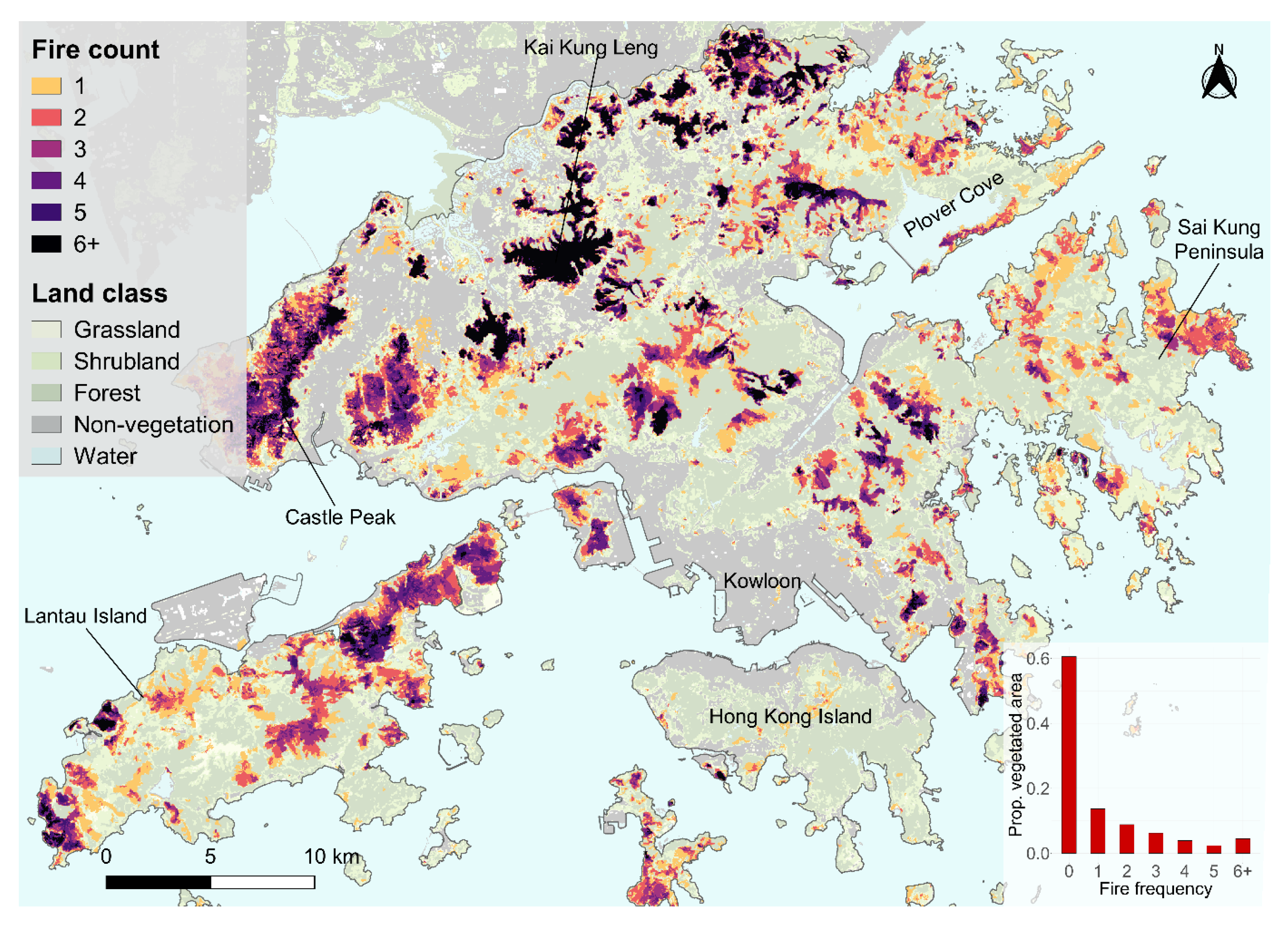
3.3. Overview of the Fire Regime in Hong Kong

The 34-year Landsat burn-area time series was visualized by a time-lapse video (Video S1), a fire-frequency map (Figure 9), and summary graphs (Figure 10), which together revealed spatial and temporal patterns of fires in Hong Kong. The total detected burnt area was 909.9 km², against a total vegetated area of 728.4 km², which would amount to 125% of land if fires never occurred at the same location twice. In reality, repeated fires often occur. In fact, most (60.6%, or 441.1 km²) of the vegetated pixels were unburnt throughout the study period (Figure 9), while a majority of burnt pixels (65.4%) burnt more than once, suggesting strongly positive fire-vegetation feedback dynamics. Spatially, the forested vegetation on the highly urbanized Hong Kong Island appeared to be better protected and was the least-burnt region in the study area. Grasslands and shrublands on the Sai Kung Peninsula and near Plover Cove burnt frequently before 2000 but has since seen reduced fire occurrence (Video S1), likely due to a drop in rural population and associated land-management practices. Vegetation in the Northern District, along with the mountains near Kai Kung Leng and Castle Peak, burnt frequently across the entire study period, with many of the grassy slopes burning ≥ 6 times in the last 34 years (Video S1 and Figure 9).

Fires have become less prevalent over time. Fire-affected area dropped from 20–50 km² per fire season before 2000 to 5–25 km² per fire season in 2008–2020 (Figure 10a). The trend highlights an overall success in fire suppression in Hong Kong. Fire prevalence oscillated strongly, usually in 2–3-year cycles, possibly due to fuel accumulation entrained by weather patterns. Despite cool ambient temperatures, most fires broke out in the drier autumn and winter months (October–January). Notably, albeit with the delay in detection (Figure 9), the peaks in fire occurrence could be attributed to the traditional Ching Ming (early April) and Chung Yeung (October) Festivals (Figure 10b). During these festivals, locals clear vegetation around graves, light candles, and burn joss paper to pay respect to their ancestors, which often led to spillover fires if weather conditions are dry [7,60].

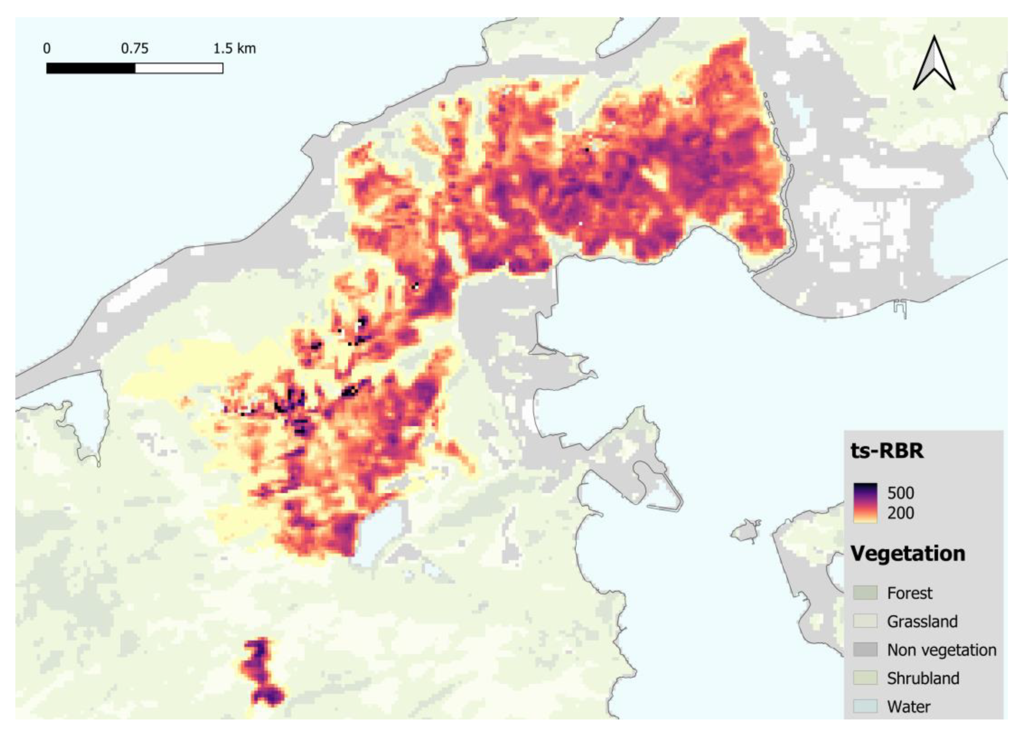
3.4. Burn Severity Estimation

Burn severity estimated by ts-RBR was effectively relativized across different types of vegetation. Figure 11 demonstrates burn severity estimated by ts-RBR over a burnt patch near Discovery Bay, Lantau Island in 2004. No field surveys were carried out to verify ts-RBR patterns observed, but we generally found lower burn severity near the edge and patchy distribution of severity across the rest of the burn area. ts-RBR values typically ranged between 50–500. With a large sample size (n = 179,713), the vegetation type was found to significantly affect ts-RBR (F = 300, p < 0.001, ANOVA). However, the effect sizes were very small (Figure S2). Ω² of the model shows that the vegetation type only accounts for 0.3% of the variance in ts-RBR, indicating that the metric was effectively relativized and ts-RBR values were comparable across different types of vegetation.

4. Discussion

Our LTS fire map of Hong Kong represents the first regional Landsat BA map in wet tropical/subtropical Asia that covers the full Landsat 5/7/8 time series (Table S1). It is also the first long-term Landsat BA map in the wet tropics/subtropics that incorporated estimated date of BA detection and burn severity (Table S1). When validated with government fire records, the LTS fire map was found to carry very low omission errors, omitting only 11.2% of the burnt area compared with MCD64A1 (72%) and FireCCI51 (96%). The high omission errors of MODIS-based BA maps were partially due to the low spatial resolution MODIS, as 4.1% and 18.1% of the burnt area in the ancillary dataset were found in patches that were smaller than the pixel size of FireCCI51 (250 m) and MCD64A1 (500 m), respectively. However, most of the pixels omitted (74.9% of MCD64A1 omissions and 95.7% of FireCCI51 omissions) were attributable to larger patches. Many of these fires were probably still too scattered to be readily detectable or were extinguished before the MODIS satellite returned. The results revealed the limitations of algorithms that grow BAs based on MODIS active fire data. It is also worth noting that the mean area of burnt patches detected by LTS fire (13.3 ha) was significantly smaller than the patches delineated for validation (31.1 ha) (Figure S3). Had we sampled the true size distribution of burnt patches, the omission errors of the two MODIS BA products would be even higher. While burnt patches in Hong Kong tend to be smaller than other tropical/subtropical regions due to habitat fragmentation and government fire suppression (Figure S3) [75,76], the results nonetheless highlighted the importance of incorporating higher-resolution datasets if fire histories of landscapes were to be accurately reconstructed.

LTS fire also performed well compared to Landsat-based GABAM, omitting 11.2% rather than 49.3% of burnt area while keeping commission errors low (Table 1). We do acknowledge that direct comparisons between locally trained BA maps with global datasets may lead to biases, even with independent cross-validation. However, we believe that the stark differences in accuracies could at least be partially attributed to methodological differences in preprocessing. Most existing BA mapping algorithms, including GABAM, do not directly classify pixels into binary burnt/unburnt maps. Rather, continuous proxies of BA resemblance, such as VIs, predicted burnt probabilities, or, in this study, the equivalent number of days after fire (Δτ), which are thresholded into BA products. Thresholding makes BA mapping more flexible. For instance, our study adopted the two-phase seed-growing approach proposed by Bastarrika et al. (2011) [45]. The approach elegantly incorporates spatial information into feature selection by overlaying polygons created by two thresholds, reducing both omission and commission errors (Figure 5). GABAM additionally incorporated a number of additional thresholds that could vary according to land cover [55]. However, existing approaches rarely explicitly address the issue of temporal stability. When a single set of thresholds is applied across multiple scenes in the time series, the balance between omission and commission errors can change drastically. Depending on incident sunlight and haze, some scenes have lower baseline NIR:SWIR ratios across all pixels, leading to bursts in commission errors (Figure 8c and Figure S4). Similarly, burnt pixels in a particular season can be omitted if the scenes had a high baseline of NIR:SWIR ratios. At smaller spatial-temporal scales, this issue could be avoided by preselecting Landsat scenes that are unaffected by atypical incident sunlight or atmospheric effects. In fact, most existing Landsat BA maps in the wet tropics and subtropics operate on preselected scenes (Table S1). However, we believe that scene preselection makes algorithms difficult to generalize. Moreover, the high cloud cover in the wet tropics and subtropics means that it is not uncommon for seasons to be only covered by a single atypical scene. GABAM addressed this by adding more thresholds and adopting relatively conservative thresholds [55]. Even so, atypical Landsat 7 scenes still caused bursts in commission errors in the GABAM time series (Figure 8c). In LTS fire, we developed a new weighted histogram matching approach to address this issue (Section 2.3, Figure 2). By uniformizing Landsat scenes, we effectively minimized these sudden bursts in commission errors (Figure S4). The preprocessing also ensured that the model performance was comparable across imagery collected by different sensors in Landsat 5, 7, and 8. LTS fire did not perform significantly worse for known burnt patches in the Landsat 5 era, even when most training pixels were derived from Landsat 7/8 years. We also did not observe any significant changes in size distribution of detected patches across time, indicating that LTS fire was equally sensitive to smaller features when applied to Landsat 5 data (Figure S5). This temporal stability allowed us to adopt less conservative thresholds when mapping BAs, which in turn significantly suppressed omission errors without the expense in commission errors (Table 1). One potential concern of weighted histogram matching is the possibility of the process smoothing out BA features when burnt pixels are adjusted to match the histogram of the unburnt reference composite, increasing omission errors. Since burnt pixels are scarce relative to unburnt pixels, we found this to be a relatively minor issue in our study site. The benefits of temporal stability, which suppressed omission errors by allowing for less conservative thresholds, significantly outweighed the potential increase in omissions caused by smoothing (Table 1). Nevertheless, minor changes to the algorithm would probably be needed if burn patches are large enough to span significant portions of Landsat scenes. In this case, the function to adjust pixel brightness could be derived from vegetated pixels only, then applied to both vegetated areas and potential burnt patches. This would uniformize the scenes without forcing output Landsat scenes with large burnt patches to have the exact histogram of the unburnt reference composite.

Another important addition to the pipeline is the coupling of date-traceable compositing with iterative polygon merging to estimate dates of detection of BA polygons. Date stamps facilitate temporal analyses on fire occurrence (Figure 10) to be carried out at a level of detail previously only available in MODIS-based datasets or after cross-validation with government fire records [20,29,77]. Considering the low temporal resolution of Landsat (16 days), the fact that the algorithm dated most polygons within a month and 76.9% of polygons within two months of the actual fire exceeded expectations (Figure 7). This is achieved by incorporating the full time series, including many heavily clouded or hazy scenes, when creating the date-traceable composites (Section 2.3, Figure 2). These min-NBR composites preserved the dates of pixels once they were captured by Landsat, even when many BAs were at the time only partially visible through cloud gaps or amongst Landsat 7 scan lines. Creating a set of criteria to decide how these dated BA polygons should be merged was by far the most challenging part in fire date estimation. Specifically, two separate issues were in play. Firstly, pixels burn repeatedly (Figure 9). The minimum interval between two separate fires depends mainly on landcover type and the rate of fuel accumulation. In Hong Kong, grassy slopes could occasionally burn repeatedly within a year, but apart from rare exceptions, repeated fires were usually more than a year apart. Hence, we designed the iterative polygon merging process such that overlapping polygons were merged if seed-polygon dates were ± 1 season apart. We are aware that the rate of revegetation and fuel accumulation can be vastly different in other biomes. In regions with rapid revegetation, quick fuel accumulation, and frequent repeated fires, the definitions of seasons would have to be shortened, while in regions with sluggish revegetation, slow fuel accumulation, and infrequent repeated fires, polygons dated more than one season apart ought to be merged. The second issue concerns neighboring burnt areas. Even if pixels do not burn repeatedly, two separate burnt patches ± 1 season apart could intersect at the border. It is challenging to determine whether intersecting patches with different dates of detection were (1) Caused by the same fire but were scattered across more than one Landsat scenes; or (2) Caused by two different fires. In this study, we did not make this distinction, and, occasionally, BA polygons were dated earlier than the actual fire (negative time differences in Figure 7). However, we did adopt an area-based algorithm such that if two separate polygons were wrongfully merged, at least the fire dates of large patches would not be dragged by much smaller ones. A solution to this issue is to extract additional data from the Landsat scenes before they were made into seasonal min-NBR composites, but that would likely come at the expense of computational time. Finally, it is worth noting that the accuracy of estimated dates depends on the temporal resolution of the input Landsat time series. In earlier years with only Landsat 5 data, or in cloudy seasons, the estimated dates of detection would unavoidably be less accurate. Nevertheless, the estimated dates of BA detection at its current form should be robust enough for a large range of ecological applications, such as how seasonal weather patterns affect fire susceptibility or post-fire recovery in the wet tropics and subtropics.

The LTS fire pipeline also incorporated the time series relativized burn ratio (ts-RBR) as a burn severity metric. The index was developed as a variant of relativized burn ratio (RBR) [72] but made robust against poor data quality by considering multiple pre- and post-fire scenes in the Landsat time series simultaneously (Section 2.6 and Figure 11). The search for appropriate remotely sensed indices to represent burn severity has received much attention in recent years. Earlier studies often directly used NBR (Equation (1)) or its difference pre- and post-fire, dNBR (Equation (2)), to estimate burn severity [78,79,80,81]. However, these metrics do not address the issue of shifting NBR baselines across different vegetation types. Grasslands or short shrublands often have lower absolute NBR and, hence, smaller dNBR values compared to forests, regardless of relative severity [20,72]. Recognizing these issues, many studies started adopting relativized dNBR, or RdNBR, to estimate burn severity [9,25,35,82,83]. In recent years, the robustness of RdNBR in accurately quantifying burn severity has come into question [72,81]. In particular, Parks et al. (2014) [72] pointed out that RdNBR is mathematically unstable and introduced RBR (Equation (3)) as a more reliable alternative that better echoed field-measured severity [72]. In this study, we hope to contribute to this discussion by proposing the use of ts-RBR in areas where single cloudless pre- and post-fire scenes are not readily available. By consulting multiple pre- and post-fire scenes, the approach maximizes the chance of reconstructing burn severity patterns that would otherwise be partially occluded by clouds and artifacts. We are aware that more sophisticated methods have been developed to better match remotely sensed fire severity with a field-measured composite burn index (CBI). However, many are contingent upon calibrations to local climate regimes [20,84]. This makes such approaches less generalizable, especially in the tropics/subtropics where data needed to calibrate the burn severity models are not readily available. Therefore, we decided to make less assumptions and adopt ts-RBR in the pipeline instead. Finally, it is important to note that RBR was mainly validated in the US [72]. The caveats of applying the metric outside its validation window would also apply to ts-RBR. Moreover, ts-RBR should be viewed as a method to obtain RBR from time series data, not as a new and fully validated severity metric. Nevertheless, we believe that the severity data provided here could act as a rough baseline for future ecological studies, and we hope that this could elicit further discussions to find the best practice in estimating burn severity across wet tropical and subtropical BAs.

Looking into the future, we believe that the LTS fire pipeline can be adopted more widely to provide ecologically relevant BA maps for researchers. Our results demonstrated how over three decades of fire history could be accurately reconstructed using Landsat data in a wet subtropical landscape with a highly diverse vegetation structure (Figure 9 and Figure 10). The seasonal, decadal, and spatial trends that we observed, such as the overall changes in fire abundance and seasonal peaks near local festivals, closely echoes what was reported by local ecological studies in Hong Kong [7,60,85]. Compared with most previous studies on Landsat/Sentinel BA mapping the wet tropics and subtropics, LTS fire is comparatively close to being data agnostic as it does not require preselection of Landsat scenes (Table S1). We do, nonetheless, recognize five areas where the LTS fire pipeline needs further modification before it could be applied more widely. Firstly, as mentioned above, the weighted histogram matching approach might need slight adjustments if the area of interest contains very large BAs. Secondly, we adopted Δτ, the equivalent number of days after fire, as the proxy for pixel resemblance to BAs. While Δτ is a more information-rich proxy and should be adopted, if possible, it cannot be derived from training datasets without exact fire dates. An alternative that trains RF models from binary burnt/unburnt pixels may be useful. Thirdly, the two thresholds used to create seed and growth polygons are currently chosen by eyeballing the threshold-error curves (Figure 5). A mathematical expression to derive the threshold from the curves will make the pipeline more automatable. Fourthly, as briefly discussed above, the rate of revegetation and fuel accumulation affects the minimum temporal interval between fires. In this study, the Landsat scenes were grouped by seasons, and resulting BA polygons are merged accordingly. An option to change seasonal boundaries and merging criteria based on the rate of revegetation would make the pipeline more generalizable. Finally, the current pipeline was mainly written in R and implemented in a local cluster. While R provides ample flexibility for pipeline development, a translation that allows the pipeline to be implemented on cloud computing platforms such as GEE would greatly lift limitations in computational capacity. Overall, these five areas of future work are not insurmountable. In addition to the compilation of BA training data, such as the newly developed Burned Area Reference Database (BARD) [61], we believe that the LTS fire pipeline can be a step toward creating a new generation of Landsat-based BA maps in the wet tropics and subtropics. By providing relevant and specific information on thousands of BAs across decadal time scales, these maps will bridge the missing link between remotely sensed and field data, providing a new bedrock for tropical fire ecology.

5. Conclusions

A 34-year Landsat-based BA time series was created to reconstruct the fire history of Hong Kong by recording the location, date, and severity of burnt patches. To generate the product, a new BA detection pipeline was developed and tested on the challenging wet subtropical landscape where high cloud cover, diverse habitat types, and rapid revegetation commonly obscures BAs. The map successfully captured the fire regime of the area at a level of detail unmatched by existing global satellite-based burn-area maps. A wider availability of such long-term fire-severity maps with fine temporal and spatial resolution will greatly benefit studies in fire ecology, global climate modelling, and fire management.

References

1. Marlon, J.R.; Bartlein, P.J.; Gavin, D.G.; Long, C.J.; Anderson, R.S.; Briles, C.E.; Brown, K.J.; Colombaroli, D.; Hallett, D.J.; Power, M.J.; et al. Long-term perspective on wildfires in the western. Proc. Natl. Acad. Sci. USA 2012, 109, E535–E543. [Google Scholar] [CrossRef] [PubMed] [Green Version]
2. Fernandes, K.; Baethgen, W.; Bernardes, S.; DeFries, R.; DeWitt, D.G.; Goddard, L.; Lavado, W.; Lee, D.E.; Padoch, C.; Pinedo-Vasquez, M.; et al. North Tropical Atlantic influence on western Amazon fire season variability. Geophys. Res. Lett. 2011, 38, 12701. [Google Scholar] [CrossRef] [Green Version]
3. Aragão, L.E.O.C.; Anderson, L.O.; Fonseca, M.G.; Rosan, T.M.; Vedovato, L.B.; Wagner, F.H.; Silva, C.V.J.; Silva Junior, C.H.L.; Arai, E.; Aguiar, A.P.; et al. 21st Century drought-related fires counteract the decline of Amazon deforestation carbon emissions. Nat. Commun. 2018, 9, 536. [Google Scholar] [CrossRef] [Green Version]
4. Silva, C.V.J.; Aragão, L.E.O.C.; Young, P.J.; Espirito-Santo, F.; Berenguer, E.; Anderson, L.O.; Brasil, I.; Pontes-Lopes, A.; Ferreira, J.; Withey, K.; et al. Estimating the multi-decadal carbon deficit of burned Amazonian forests. Environ. Res. Lett. 2020, 15, 114023. [Google Scholar] [CrossRef]
5. Abatzoglou, J.T.; Williams, A.P.; Barbero, R. Global Emergence of Anthropogenic Climate Change in Fire Weather Indices. Geophys. Res. Lett. 2019, 46, 326–336. [Google Scholar] [CrossRef] [Green Version]
6. Tien Bui, D.; Le, K.-T.; Nguyen, V.; Le, H.; Revhaug, I. Tropical Forest Fire Susceptibility Mapping at the Cat Ba National Park Area, Hai Phong City, Vietnam, Using GIS-Based Kernel Logistic Regression. Remote Sens. 2016, 8, 347. [Google Scholar] [CrossRef] [Green Version]
7. Chau, K.L. The Ecology of Fire in Hong Kong. Ph.D. Thesis, The University of Hong Kong, Hong Kong, China, 1994. [Google Scholar]
8. Johnstone, J.F.; Hollingsworth, T.N.; Chapin, F.S.; Mack, M.C. Changes in fire regime break the legacy lock on successional trajectories in Alaskan boreal forest. Glob. Chang. Biol. 2010, 16, 1281–1295. [Google Scholar] [CrossRef]
9. Kemp, K.B.; Higuera, P.E.; Morgan, P. Fire legacies impact conifer regeneration across environmental gradients in the U.S. northern Rockies. Landsc. Ecol. 2016, 31, 619–636. [Google Scholar] [CrossRef]
10. Tepley, A.J.; Thomann, E.; Veblen, T.T.; Perry, G.L.W.; Holz, A.; Paritsis, J.; Kitzberger, T.; Anderson-Teixeira, K.J. Influences of fire–vegetation feedbacks and post-fire recovery rates on forest landscape vulnerability to altered fire regimes. J. Ecol. 2018, 106, 1925–1940. [Google Scholar] [CrossRef] [Green Version]
11. Tansey, K.; Grégoire, J.M.; Defourny, P.; Leigh, R.; Pekel, J.F.; van Bogaert, E.; Bartholomé, E. A new, global, multi-annual (2000–2007) burnt area product at 1 km resolution. Geophys. Res. Lett. 2008, 35. [Google Scholar] [CrossRef]
12. Simon, M.; Plummer, S.; Fierens, F.; Hoelzemann, J.J.; Arino, O. Burnt area detection at global scale using ATSR-2: The GLOBSCAR products and their qualification. J. Geophys. Res. Atmos. 2004, 109. [Google Scholar] [CrossRef]
13. Chuvieco, E.; Mouillot, F.; van der Werf, G.R.; San Miguel, J.; Tanasse, M.; Koutsias, N.; García, M.; Yebra, M.; Padilla, M.; Gitas, I.; et al. Historical background and current developments for mapping burned area from satellite Earth observation. Remote Sens. Environ. 2019, 225, 45–64. [Google Scholar] [CrossRef]
14. Giglio, L.; Boschetti, L.; Roy, D.P.; Humber, M.L.; Justice, C.O. The Collection 6 MODIS burned area mapping algorithm and product. Remote Sens. Environ. 2018, 217, 72–85. [Google Scholar] [CrossRef] [PubMed]
15. Lizundia-Loiola, J.; Otón, G.; Ramo, R.; Chuvieco, E. A spatio-temporal active-fire clustering approach for global burned area mapping at 250 m from MODIS data. Remote Sens. Environ. 2020, 236, 111493. [Google Scholar] [CrossRef]
16. Archibald, S.; Scholes, R.J.; Roy, D.P.; Roberts, G.; Boschetti, L. Southern African fire regimes as revealed by remote sensing. Int. J. Wildl. Fire 2010, 19, 861–878. [Google Scholar] [CrossRef] [Green Version]
17. Chuvieco, E.; Aguado, I.; Salas, J.; García, M.; Yebra, M.; Oliva, P. Satellite Remote Sensing Contributions to Wildland Fire Science and Management. Curr. For. Rep. 2020, 6, 81–96. [Google Scholar] [CrossRef]
18. Lizundia-Loiola, J.; Pettinari, M.L.; Chuvieco, E. Temporal Anomalies in Burned Area Trends: Satellite Estimations of the Amazonian 2019 Fire Crisis. Remote Sens. 2020, 12, 151. [Google Scholar] [CrossRef] [Green Version]
19. Zheng, B.; Ciais, P.; Chevallier, F.; Chuvieco, E.; Chen, Y.; Yang, H. Increasing forest fire emissions despite the decline in global burned area. Sci. Adv. 2021, 7, eabh2646. [Google Scholar] [CrossRef]
20. Szpakowski, D.M.; Jensen, J.L.R. A Review of the Applications of Remote Sensing in Fire Ecology. Remote Sens. 2019, 11, 2638. [Google Scholar] [CrossRef] [Green Version]
21. Padilla, M.; Stehman, S.V.; Ramo, R.; Corti, D.; Hantson, S.; Oliva, P.; Alonso-Canas, I.; Bradley, A.V.; Tansey, K.; Mota, B.; et al. Comparing the accuracies of remote sensing global burned area products using stratified random sampling and estimation. Remote Sens. Environ. 2015, 160, 114–121. [Google Scholar] [CrossRef] [Green Version]
22. Franquesa, M.; Lizundia-Loiola, J.; Stehman, S.V.; Chuvieco, E. Using long temporal reference units to assess the spatial accuracy of global satellite-derived burned area products. Remote Sens. Environ. 2022, 269, 112823. [Google Scholar] [CrossRef]
23. Boschetti, L.; Roy, D.P.; Giglio, L.; Huang, H.; Zubkova, M.; Humber, M.L. Global validation of the collection 6 MODIS burned area product. Remote Sens. Environ. 2019, 235, 111490. [Google Scholar] [CrossRef] [PubMed]
24. Humber, M.L.; Boschetti, L.; Giglio, L.; Justice, C.O. Spatial and temporal intercomparison of four global burned area products. Int. J. Digit. Earth 2019, 12, 460–484. [Google Scholar] [CrossRef] [PubMed] [Green Version]
25. Busby, S.U.; Moffett, K.B.; Holz, A. High-severity and short-interval wildfires limit forest recovery in the Central Cascade Range. Ecosphere 2020, 11, e03247. [Google Scholar] [CrossRef]
26. Kibler, C.L.; Parkinson, A.-M.L.; Peterson, S.H.; Roberts, D.A.; D’Antonio, C.M.; Meerdink, S.K.; Sweeney, S.H. Monitoring Post-Fire Recovery of Chaparral and Conifer Species Using Field Surveys and Landsat Time Series. Remote Sens. 2019, 11, 2963. [Google Scholar] [CrossRef] [Green Version]
27. Polychronaki, A.; Gitas, I.; Veraverbeke, S.; Debien, A. Evaluation of ALOS PALSAR Imagery for Burned Area Mapping in Greece Using Object-Based Classification. Remote Sens. 2013, 5, 5680–5701. [Google Scholar] [CrossRef] [Green Version]
28. Fernández-García, V.; Quintano, C.; Taboada, A.; Marcos, E.; Calvo, L.; Fernández-Manso, A. Remote Sensing Applied to the Study of Fire Regime Attributes and Their Influence on Post-Fire Greenness Recovery in Pine Ecosystems. Remote Sens. 2018, 10, 733. [Google Scholar] [CrossRef] [Green Version]
29. Hawbaker, T.J.; Vanderhoof, M.K.; Beal, Y.J.; Takacs, J.D.; Schmidt, G.L.; Falgout, J.T.; Williams, B.; Fairaux, N.M.; Caldwell, M.K.; Picotte, J.J.; et al. Mapping burned areas using dense time-series of Landsat data. Remote Sens. Environ. 2017, 198, 504–522. [Google Scholar] [CrossRef]
30. Vanderhoof, M.K.; Fairaux, N.; Beal, Y.J.G.; Hawbaker, T.J. Validation of the USGS Landsat Burned Area Essential Climate Variable (BAECV) across the conterminous United States. Remote Sens. Environ. 2017, 198, 393–406. [Google Scholar] [CrossRef]
31. Goodwin, N.R.; Collett, L.J. Development of an automated method for mapping fire history captured in Landsat TM and ETM + time series across Queensland, Australia. Remote Sens. Environ. 2014, 148, 206–221. [Google Scholar] [CrossRef]
32. Tompoulidou, M.; Stefanidou, A.; Grigoriadis, D.; Dragozi, E.; Stavrakoudis, D.; Gitas, I.Z. The Greek National Observatory of Forest Fires (NOFFi). IOP Conf. Ser. Earth Environ. Sci. 2016, 9688, 199–207. [Google Scholar]
33. Abatzoglou, J.T.; Battisti, D.S.; Williams, A.P.; Hansen, W.D.; Harvey, B.J.; Kolden, C.A. Projected increases in western US forest fire despite growing fuel constraints. Commun. Earth Environ. 2021, 2, 227. [Google Scholar] [CrossRef]
34. Hagmann, R.K.; Hessburg, P.F.; Prichard, S.J.; Povak, N.A.; Brown, P.M.; Fulé, P.Z.; Keane, R.E.; Knapp, E.E.; Lydersen, J.M.; Metlen, K.L.; et al. Evidence for widespread changes in the structure, composition, and fire regimes of western North American forests. Ecol. Appl. 2021, 31, e02431. [Google Scholar] [CrossRef] [PubMed]
35. Mallek, C.; Safford, H.; Viers, J.; Miller, J. Modern departures in fire severity and area vary by forest type, Sierra Nevada and southern Cascades, California, USA. Ecosphere 2013, 4, art153. [Google Scholar] [CrossRef]
36. Gibson, R.; Danaher, T.; Hehir, W.; Collins, L. A remote sensing approach to mapping fire severity in south-eastern Australia using sentinel 2 and random forest. Remote Sens. Environ. 2020, 240, 111702. [Google Scholar] [CrossRef]
37. Wimberly, M.C.; Reilly, M.J. Assessment of fire severity and species diversity in the southern Appalachians using Landsat TM and ETM+ imagery. Remote Sens. Environ. 2007, 108, 189–197. [Google Scholar] [CrossRef] [Green Version]
38. Daldegan, G.A.; Roberts, D.A.; de Figueiredo Ribeiro, F. Spectral mixture analysis in Google Earth Engine to model and delineate fire scars over a large extent and a long time-series in a rainforest-savanna transition zone. Remote Sens. Environ. 2019, 232, 111340. [Google Scholar] [CrossRef]
39. Cochrane, M.A.; Moran, C.J.; Wimberly, M.C.; Baer, A.D.; Finney, M.A.; Beckendorf, K.L.; Eidenshink, J.; Zhu, Z.; Cochrane, M.A.; Moran, C.J.; et al. Estimation of wildfire size and risk changes due to fuels treatments. Int. J. Wildl. Fire 2012, 21, 357–367. [Google Scholar] [CrossRef] [Green Version]
40. Bright, B.C.; Hudak, A.T.; Kennedy, R.E.; Braaten, J.D.; Henareh Khalyani, A. Examining post-fire vegetation recovery with Landsat time series analysis in three western North American forest types. Fire Ecol. 2019, 15, 8. [Google Scholar] [CrossRef] [Green Version]
41. Frazier, R.J.; Coops, N.C.; Wulder, M.A.; Hermosilla, T.; White, J.C. Analyzing spatial and temporal variability in short-term rates of post-fire vegetation return from Landsat time series. Remote Sens. Environ. 2018, 205, 32–45. [Google Scholar] [CrossRef]
42. Mahood, A.L.; Balch, J.K. Repeated fires reduce plant diversity in low-elevation Wyoming big sagebrush ecosystems (1984–2014). Ecosphere 2019, 10, e02591. [Google Scholar] [CrossRef] [Green Version]
43. Boschetti, L.; Stehman, S.V.; Roy, D.P. A stratified random sampling design in space and time for regional to global scale burned area product validation. Remote Sens. Environ. 2016, 186, 465–478. [Google Scholar] [CrossRef] [PubMed]
44. Mallinis, G.; Koutsias, N. Comparing ten classification methods for burned area mapping in a Mediterranean environment using Landsat TM satellite data. Int. J. Remote Sens. 2012, 33, 4408–4433. [Google Scholar] [CrossRef]
45. Bastarrika, A.; Chuvieco, E.; Martín, M.P. Mapping burned areas from landsat TM/ETM+ data with a two-phase algorithm: Balancing omission and commission errors. Remote Sens. Environ. 2011, 115, 1003–1012. [Google Scholar] [CrossRef]
46. Nelson, K.J.; Connot, J.; Peterson, B.; Martin, C. The LANDFIRE Refresh Strategy: Updating the National Dataset. Fire Ecol. 2013, 9, 80–101. [Google Scholar] [CrossRef]
47. Huang, C.; Goward, S.N.; Masek, J.G.; Gao, F.; Vermote, E.F.; Thomas, N.; Schleeweis, K.; Kennedy, R.E.; Zhu, Z.; Eidenshink, J.C.; et al. Development of time series stacks of Landsat images for reconstructing forest disturbance history. Int. J. Digit. Earth 2009, 2, 195–218. [Google Scholar] [CrossRef]
48. Mitri, G.H.; Gitas, I.Z. A semi-automated object-oriented model for burned area mapping in the Mediterranean region using Landsat-TM imagery. Int. J. Wildl. Fire 2004, 13, 367. [Google Scholar] [CrossRef]
49. Hudak, A.T.; Brockett, B.H. Mapping fire scars in a southern African savannah using Landsat imagery. Int. J. Remote Sens. 2010, 25, 3231–3243. [Google Scholar] [CrossRef]
50. Bowman, D.M.J.S.; Zhang, Y.; Walsh, A.; Williams, R.J. Experimental comparison of four remote sensing techniques to map tropical savanna fire-scars using Landsat-TM imagery. Int. J. Wildl. Fire 2003, 12, 341–348. [Google Scholar] [CrossRef]
51. Liu, J.; Heiskanen, J.; Maeda, E.E.; Pellikka, P.K.E. Burned area detection based on Landsat time series in savannas of southern Burkina Faso. Int. J. Appl. Earth Obs. Geoinf. 2018, 64, 210–220. [Google Scholar] [CrossRef] [Green Version]
52. Brun, P.; Zimmermann, N.E.; Hari, C.; Pellissier, L.; Karger, D.N. Global climate-related predictors at kilometre resolution for the past and future. Earth Syst. Sci. Data Discuss. 2022, 2022, 5573–5603. [Google Scholar] [CrossRef]
53. Asner, G.P. Cloud cover in Landsat observations of the Brazilian Amazon. Int. J. Remote Sens. 2001, 22, 3855–3862. [Google Scholar] [CrossRef]
54. Roteta, E.; Bastarrika, A.; Padilla, M.; Storm, T.; Chuvieco, E. Development of a Sentinel-2 burned area algorithm: Generation of a small fire database for sub-Saharan Africa. Remote Sens. Environ. 2019, 222, 1–17. [Google Scholar] [CrossRef]
55. Long, T.; Zhang, Z.; He, G.; Jiao, W.; Tang, C.; Wu, B.; Zhang, X.; Wang, G.; Yin, R. 30 m resolution global annual burned area mapping based on landsat images and Google Earth Engine. Remote Sens. 2019, 11, 489. [Google Scholar] [CrossRef] [Green Version]
56. Hong Kong Observatory Hong Kong Observatory. Available online: https://www.hko.gov.hk/contente.htm (accessed on 10 November 2019).
57. Dudgeon, D.; Corlett, R. The Ecology and Biodiversity of Hong Kong; Joint Publishing (Hong Kong) Ltd.: Hong Kong, China, 2004. [Google Scholar]
58. Kwong, I.H.Y.; Wong, F.K.K.; Fung, T.; Liu, E.K.Y.; Lee, R.H.; Ng, T.P.T. A multi-stage approach combining very high-resolution satellite image, gis database and post-classification modification rules for habitat mapping in Hong Kong. Remote Sens. 2022, 14, 67. [Google Scholar] [CrossRef]
59. Boschetti, L.; Roy, D.P.; Justice, C.O. International Global Burned Area Satellite Product Validation Protocol Part—Production and Standardization of Validation Reference Data; Committee on Earth Observation Satellites: Maryland, MD, USA, 2009; pp. 1–11. Available online: https://lpvs.gsfc.nasa.gov/PDF/BurnedAreaValidationProtocol.pdf (accessed on 12 September 2022).
60. Chan, W.-W.E. A Feasibility Study of Hillfire Management in Hong Kong Country Parks Using GIS Analysis. Master’s Thesis, University of Hong Kong, Hong Kong, China, 2005. [Google Scholar]
61. Franquesa, M.; Vanderhoof, M.K.; Stavrakoudis, D.; Gitas, I.Z.; Roteta, E.; Padilla, M.; Chuvieco, E. Development of a standard database of reference sites for validating global burned area products. Earth Syst. Sci. Data 2020, 12, 3229–3246. [Google Scholar] [CrossRef]
62. Abbas, S.; Nichol, J.E.; Fischer, G.A. A 70-year perspective on tropical forest regeneration. Sci. Total Environ. 2016, 544, 544–552. [Google Scholar] [CrossRef]
63. Leutner, B.; Horning, N.; Schwalb-Willmann, J.; Hijmans, R.J. Rstoolbox. R Package Version 0.2.6. 2019. Available online: https://github.com/bleutner/RStoolbox (accessed on 1 February 2021).
64. R Core Team R: A Language and Environment for Statistical Computing. 2021. Available online: https://www.scirp.org/(S(czeh2tfqw2orz553k1w0r45))/reference/referencespapers.aspx?referenceid=3131254 (accessed on 1 February 2021).
65. Penha, T.V.; Körting, T.S.; Fonseca, L.M.G.; Silva Júnior, C.H.L.; Pletsch, M.A.J.S.; Anderson, L.O.; Morelli, F. Burned Area Detection in the Brazilian Amazon using Spectral Indices and GEOBIA. Rev. Bras. Cartogr. 2020, 72, 253–269. [Google Scholar] [CrossRef]
66. Wu, C. Normalized spectral mixture analysis for monitoring urban composition using ETM+ imagery. Remote Sens. Environ. 2004, 93, 480–492. [Google Scholar] [CrossRef]
67. Chan, A.H.Y.; Barnes, C.; Swinfield, T.; Coomes, D.A. Monitoring ash dieback (Hymenoscyphus fraxineus) in British forests using hyperspectral remote sensing. Remote Sens. Ecol. Conserv. 2021, 7, 306–320. [Google Scholar] [CrossRef]
68. Gaveau, D.L.A.; Descals, A.; Salim, M.A.; Sheil, D.; Sloan, S. Refined burned-area mapping protocol using Sentinel-2 data increases estimate of 2019 Indonesian burning. Earth Syst. Sci. Data 2021, 13, 5353–5368. [Google Scholar] [CrossRef]
69. Breiman, L.; Cutler, A.; Liaw, A.; Wiener, M. Package ‘Randomforest’; University of California, Berkeley: Berkeley, CA, USA, 2018. [Google Scholar]
70. Khoshgoftaar, T.M.; Golawala, M.; Van Hulse, J. An empirical study of learning from imbalanced data using random forest. Proc.—Int. Conf. Tools Artif. Intell. ICTAI 2007, 2, 310–317. [Google Scholar]
71. Pebesma, E.J. Simple features for R: Standardized support for spatial vector data. R J. 2018, 10, 439. [Google Scholar] [CrossRef] [Green Version]
72. Parks, S.A.; Dillon, G.K.; Miller, C. A New Metric for Quantifying Burn Severity: The Relativized Burn Ratio. Remote Sens. 2014, 6, 1827–1844. [Google Scholar] [CrossRef] [Green Version]
73. QGIS Development Team QGIS Geographic Information System. 2021. Available online: https://www.qgis.org/en/site/ (accessed on 13 June 2021).
74. Tomar, S. Converting video formats with FFmpeg. Linux J. 2006, 2006, 10. [Google Scholar]
75. Morton, D.C.; DeFries, R.S.; Nagol, J.; Souza, C.M.; Kasischke, E.S.; Hurtt, G.C.; Dubayah, R. Mapping canopy damage from understory fires in Amazon forests using annual time series of Landsat and MODIS data. Remote Sens. Environ. 2011, 115, 1706–1720. [Google Scholar] [CrossRef] [Green Version]
76. Hantson, S.; Pueyo, S.; Chuvieco, E.; Hantson, S.; Pueyo, S.; Chuvieco, E. Global fire size distribution: From power law to log-normal. Int. J. Wildl. Fire 2016, 25, 403–412. [Google Scholar] [CrossRef]
77. Ryan, K.C.; Opperman, T.S. LANDFIRE—A national vegetation/fuels data base for use in fuels treatment, restoration, and suppression planning. For. Ecol. Manage 2013, 294, 208–216. [Google Scholar] [CrossRef] [Green Version]
78. Key, C.H.; Benson, N.C. Landscape Assessment (LA). 2006. Available online: http://gsp.humboldt.edu/OLM/Courses/GSP_216/labs/rmrs_gtr164_13_land_assess.pdf (accessed on 24 September 2021).
79. Cocke, A.E.; Fulé, P.Z.; Crouse, J.E. Comparison of burn severity assessments using Differenced Normalized Burn Ratio and ground data. Int. J. Wildl. Fire 2005, 14, 189–198. [Google Scholar] [CrossRef] [Green Version]
80. Escuin, S.; Navarro, R.; Fernández, P. Fire severity assessment by using NBR (Normalized Burn Ratio) and NDVI (Normalized Difference Vegetation Index) derived from LANDSAT TM/ETM images. Int. J. Remote Sens. 2007, 29, 1053–1073. [Google Scholar] [CrossRef]
81. Soverel, N.O.; Perrakis, D.D.B.; Coops, N.C. Estimating burn severity from Landsat dNBR and RdNBR indices across western Canada. Remote Sens. Environ. 2010, 114, 1896–1909. [Google Scholar] [CrossRef]
82. Chu, T.; Guo, X. Remote Sensing Techniques in Monitoring Post-Fire Effects and Patterns of Forest Recovery in Boreal Forest Regions: A Review. Remote Sens. 2013, 6, 470–520. [Google Scholar] [CrossRef] [Green Version]
83. Miller, J.D.; Thode, A.E. Quantifying burn severity in a heterogeneous landscape with a relative version of the delta Normalized Burn Ratio (dNBR). Remote Sens. Environ. 2007, 109, 66–80. [Google Scholar] [CrossRef]
84. Parks, S.A.; Holsinger, L.M.; Voss, M.A.; Loehman, R.A.; Robinson, N.P. Mean Composite Fire Severity Metrics Computed with Google Earth Engine Offer Improved Accuracy and Expanded Mapping Potential. Remote Sens. 2018, 10, 879. [Google Scholar] [CrossRef] [Green Version]
85. Marafa, L.M.; Chau, K.C. Morphological and chemical properties of soils along a vegetation gradient affected by fire in Hong Kong. Soil Sci. 1999, 164, 683–691. [Google Scholar] [CrossRef]
Figure 1. Map showing the study area of Hong Kong. The top left panel indicates the geographical position of Hong Kong overlayed on country boundaries from Natural Earth. The land classification raster is derived from Kwong et al. (2022) [58].
Remotesensing 15 01489 g001
Figure 2. Flow chart visualizing the LTS fire pipeline. The green boxes indicate input datasets; black boxes represent actions taken; grey boxes signify intermediate products; and orange boxes show end products. Numbering corresponds to the relevant section in the methods.
Remotesensing 15 01489 g002
Figure 3. A burnt patch in degraded shrublands near Tai To Yan, Hong Kong (22°27′15.51″N, 114°6′12.55″E) demonstrating the transient nature of local BAs. The fire broke out on 14 February 2017, according to Fire Service Department records, and was manually delineated on high-resolution Google Earth satellite imagery (light blue polygon). The patch was clearly visible on the Landsat scene captured shortly after the fire (18 February 2017) but rapidly revegetated and became undistinguishable after a few months (28 July 2017 and 3 October 2017). Panels (ac) shows true colour RGB imagery recreated from the Landsat scenes, while panels (df) show NIR band as red, SWIR1 band as green, and SWIR2 band as blue. Note the importance of SWIR bands, which is used to calculate the normalized burn ratio (NBR), in enhancing the contrast of burnt patches.
Remotesensing 15 01489 g003
Figure 4. Raster showing estimated Δτ of Sai Kung Peninsula, Hong Kong (22°25′14.4″N, 114°19′51.4″E) for the summer of 1996. We trained a Random Forest model that estimated Δτ from bands in the seasonal min-NBR composites. Δτ is a proxy for burn area resemblance. A lower Δτ indicates closer resemblance to burn-area pixels, while a higher Δτ indicates closer resemblance to unburn pixels. Red and blue areas indicate the seed and growth pixels after thresholding.
Remotesensing 15 01489 g004
Figure 5. Effects of varying the Δτ threshold of summer pixels. Δτ is the predicted time interval between a fire and date of detection from Landsat, which acts as a proxy variable for burn-area resemblance. A lower Δτ indicates closer resemblance to burn-area pixels, while a higher Δτ indicates closer resemblance to unburn pixels. We trained random forest (RF) models that predicted Δτ from either (1) Landsat data that went through the entire preprocessing pipeline (PP) or (2) reflectance/VIs that had not underwent uniformization by weighted histogram matching (NPP). Different thresholds were applied to convert the continuous Δτ to binary fire/non-fire predictions. Errors of commission (unburnt pixels misclassified as burnt), pixel omission (proportion of burnt pixels missed), and patch omission (proportion of known burnt patches that had <6 correctly classified pixels) were calculated. The vertical dash lines represent the thresholds (70/160) we adopted to seed and grow fire scars in LTS fire.
Remotesensing 15 01489 g005
Figure 6. Decision tree for iterative polygon merging based on the date (T) and area (A) of seed polygons.
Remotesensing 15 01489 g006
Figure 7. Accuracy of estimated fire dates amongst LTS fire polygons. The time difference is the time (in days) between the estimated fire date in LTS fire and the date of the fire event in the governmet (FSD/AFCD) fire records.
Remotesensing 15 01489 g007
Figure 8. Comparing the burn area map produced in this study (LTSfire) with three existing global BA products, (a) FireCCI51, (b) MCD64A1, and (c) GABAM. Areas delineated by the green polygons corresponds to the areas where LTSfire agrees with the existing dataset (Denoted by Ai ∩ Bi, or grey shading, in Figure S1). Polygons with blue or orange fill represent burnt patches only detected by the existing (Bd in Figure S1) or LTSfire (Ad in Figure S1) map, respectively. Darker shades of orange represent repeated fires in the same area omitted by the existing dataset. A 2013–2014 land classification map of Hong Kong (22°16′8″N, 113°57′6″E) derived from the Landsat data is shown in the background (Chan et al. unpublished manuscript).
Remotesensing 15 01489 g008
Figure 9. Frequency of fires over different regions of Hong Kong (22°16′8″N, 113°57′6″E). Pixels were coloured according to the number of times it burnt over the 34-year study period (1987–2020). The proportions of vegetated area being burnt 0–6+ times were tallied and plotted on the bottom right panel. The background is a 2013–2014 land classification map derived from Landsat data (Chan et al. unpublished manuscript).
Remotesensing 15 01489 g009
Figure 10. Fire prevalence in Hong Kong over time. (a) The burnt area detected by LTS fire in 33 fire seasons (15 July–15 July of the next calendar year). (b) The burnt area detected by LTS fire in each calendar month over the entire study period. Note that there might be a delay between the fire and patch detection.
Remotesensing 15 01489 g010
Figure 11. Burn severity estimated by time series relativized burn ratio (ts-RBR) of two fires near Discovery Bay, Lantau Island (22°18′35.19″N, 114°0′25.95″E) in 2004. The background map is a Landsat-based vegetation map of the area in the same year (Chan et al. unpublished manuscript).
Remotesensing 15 01489 g011