High-Resolution Mapping of Soil Organic Matter at the Field Scale Using UAV Hyperspectral Images with a Small Calibration Dataset

Abstract

The rapid acquisition of high-resolution spatial distribution of soil organic matter (SOM) at the field scale is essential for precision agriculture. The UAV imaging hyperspectral technology, with its high spatial resolution and timeliness, can fill the research gap between ground-based monitoring and remote sensing. This study aimed to test the feasibility of using UAV hyperspectral data (400–1000 nm) with a small-sized calibration sample set for mapping SOM at a 1 m resolution in typical low-relief black soil areas of Northeast China. The experiment was conducted in an approximately 20 ha field. For calibration, 20 samples were collected using a 100 × 100 m grid sampling strategy, while 20 samples were randomly collected for independent validation. UAV captured hyperspectral images with a spatial resolution of 0.05 × 0.05 m. The extracted spectra within every 1 × 1 m were then averaged to represent the spectra of that grid; this procedure was also performed across the whole field. Upon applying various spectral pretreatments, including absorbance conversion, multiple scattering correction, Savitzky–Golay smoothing filtering, and first-order differentiation, the absolute maximum values of the correlation coefficients of the spectra for SOM increased from 0.41 to 0.58. Importance analysis from the optimal random forest (RF) model showed that the characterized bands of SOM were located in the 450–600 and 750–900 nm regions. When the RF model was used, the UAV hyperspectra data (UAV-RF) were able to successfully predict SOM, with an R² of 0.53 and RMSE of 1.48 g kg⁻¹. The prediction accuracy was then compared with that obtained using ordinary kriging (OK) and the RF model based on proximal sensing (PS-RF) with the same number of calibration samples. However, the OK method failed to predict the SOM accuracy (RMSE = 2.17 g kg⁻¹; R² = 0.02) due to a low sampling density. The semi-covariance function was unable to describe the spatial variability of SOM effectively. When the sampling density was increased to 50 × 50 m, OK successfully predicted SOM, with RMSE = 1.37 g kg⁻¹ and R² = 0.59, and its results were comparable to those of UAV-RF. The prediction accuracy of PS-RF was generally consistent with that of UAV-RF, with RMSE values of 1.41 g kg⁻¹ and 1.48 g kg⁻¹ and R² values of 0.57 and 0.53, respectively, which indicated that SOM prediction based on UAV-RF is feasible. Additionally, compared with the PS platforms, the UAV hyperspectral technology could simultaneously provide spectral information of tens or even hundreds of continuous bands and spatial information at the same time. This study provides a reference for further research and development of UAV hyperspectral techniques for fine-scale SOM mapping using a small number of samples.

1. Introduction

Black soil is a valuable soil and agricultural resource [1], but excess chemical fertilizers and the overuse of farmland results in a slowly thinning the cultivated layer of soil. To ensure farmland sustainability, it is important to rapidly acquire information about the topsoil [2]. Soil organic matter (SOM) contains various nutrients and retains water and fertilizer [3], which is one of the key factors affecting soil fertility. Therefore, the precise and rapid mapping of SOM is essential for precision agriculture.

The traditional acquisition of soil information is carried out mainly through expensive, environmentally hazardous, and time-consuming laboratory chemical analysis. With the development of sensor software and computer technology, researchers have focused on the measurement of soil properties using fast, pollution-free, non-destructive remote sensing and proximal sensing technologies [4,5]. Because of the mixed pixels, coarse resolution, and long revisit period, satellite-based hyperspectral data are difficult to employ in field-scale precision agriculture. Airplane-based hyperspectrum acquisition requires long planning times and high costs [6]. Compared with the above-mentioned strategies, the UAV-based hyperspectral images are easier to access and have a high resolution and low cost. This technology has been widely used in agricultural and forestry monitoring [7,8]. Visible and near-infrared (vis–NIR) proximal hyperspectral technology has shown good performances for SOM, N, and soil clay content prediction [4,9]. Several studies have compared the application of UAV-based hyperspectral data with that of satellite-based hyperspectral imaging [10,11]. However, there is limited information available on the comparison between UAV-based hyperspectral imaging and proximal hyperspectral technologies.

In soil science, UAV hyperspectral data are used for the prediction and mapping of soil salinity [11,12], soil moisture [13], and soil heavy metals [14,15]. The UAV hyperspectral technology has shown advantages in digital soil mapping (DSM) for SOM, but its application still faces many challenges in terms of spectral processing and cost reduction. First, the UAV hyperspectrum is affected by the background interference from sensors and the field environment (soil moisture, surface conditions, particle size, and other factors). Recently, the absorbance conversion, multiplicative scatter correction (MSC), Savitzky–Golay (SG), and first derivative (FD) methods have been widely applied in proximal hyperspectral pretreatments [16,17,18,19]. More practice is needed to explore spectral processing before modeling in order to achieve high-precision mapping based on UAV hyperspectral images [5].

Soil is a spatially inhomogeneous continuum with high spatial variability. To ascertain the spatial information of soil, it is necessary to conduct a farmland survey with limited resources. Soil sampling and laboratory analysis is often a time-consuming and labor-intensive process. While the use of UAV hyperspectral images in soil science is known to reduce the cost of hardware, there has been only a little bit of consideration given to how this technology could also minimize the costs associated with soil sampling. By exploring the potential of UAV hyperspectral imaging, we may find new ways to streamline the soil sampling processes and increase the efficiency in the field of soil science. The UAV hyperspectral technology is based on spectral features for prediction. Compared to interpolation-based methods, such as ordinary kriging (OK), this technology considers more information about the synoptic environment factors of soil; therefore, the UAV hyperspectral technology can obtain the same or even better mapping accuracy with a small number of sampling points compared to that obtained with interpolation-based methods.

The overall objective of this study was to explore the feasibility of using UAV imaging hyperspectra for high-precision DSM of SOM by considering a 20 ha low-relief field in the northeastern black soil area as the study area. The study focused on the following issues: (1) exploring the best preprocessing algorithms for UAV hyperspectra, (2) analyzing the characteristic bands of SOM in the UAV hyperspectrum, and (3) evaluating high-resolution DSM for SOM in a small low-relief field based on UAV hyperspectral data.

2. Materials and Methods

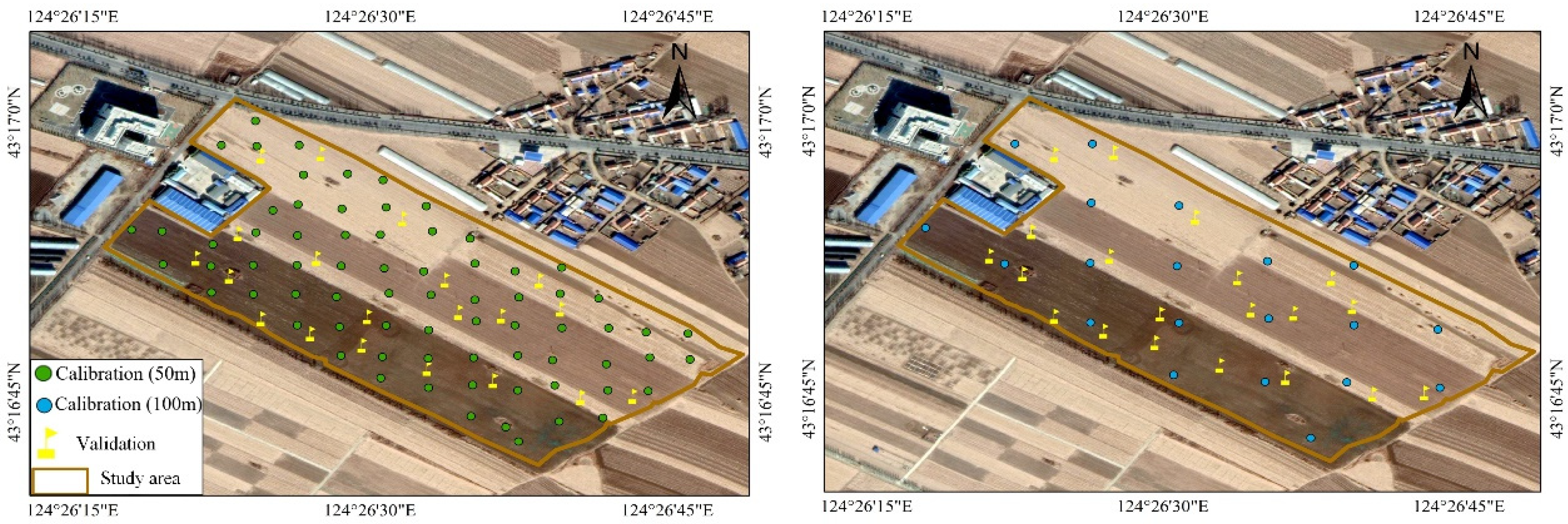
2.1. Study Sites and Experimental Design

The study region (Figure 1) is located in Lishu County, Jilin Province, China, with an area of 20 ha. This region has a monsoon climate, with an annual mean precipitation total of 553.5 mm and a mean temperature of 6.5 °C. In addition, it is characterized by a flat terrain and an average elevation of 160 m. Because of these characteristics, the region became one of three prominent black soil zones with rich SOM in the Northern Hemisphere. The main crop is soybean.

The spatial distribution of soil characteristics can be precisely determined using grid sampling [20]. In this study, grid sampling was used to select the sampling sites. The study area was divided into regular 50 × 50 m squares, and points were taken in the center of the squares (72 samples). On this basis, we raked the soil evenly to obtain soil samples with a sampling interval of 100 m and obtained 20 samples. To ensure the independence of model verification, the other 20 sampling points within the research area were randomly selected as the test set. On June 15, 2020, soil samples were collected from the surface soil layer (0–20 cm). After air drying, grinding, and screening them, SOM was determined using the Walkley–Black (WB) technique [21]. In this study, SOM prediction using UAV hyperspectroscopy images and proximal sensing data was based on sampling locations with a sampling interval of 100 m (see Section 3.2 and Section 3.3). Only the Kriging interpolation mentioned in Section 3.4 discusses the performance of the proposed method with fewer samples using the sample points, with a sampling interval of 50 m.

2.2. Hyperspectroscopy Data

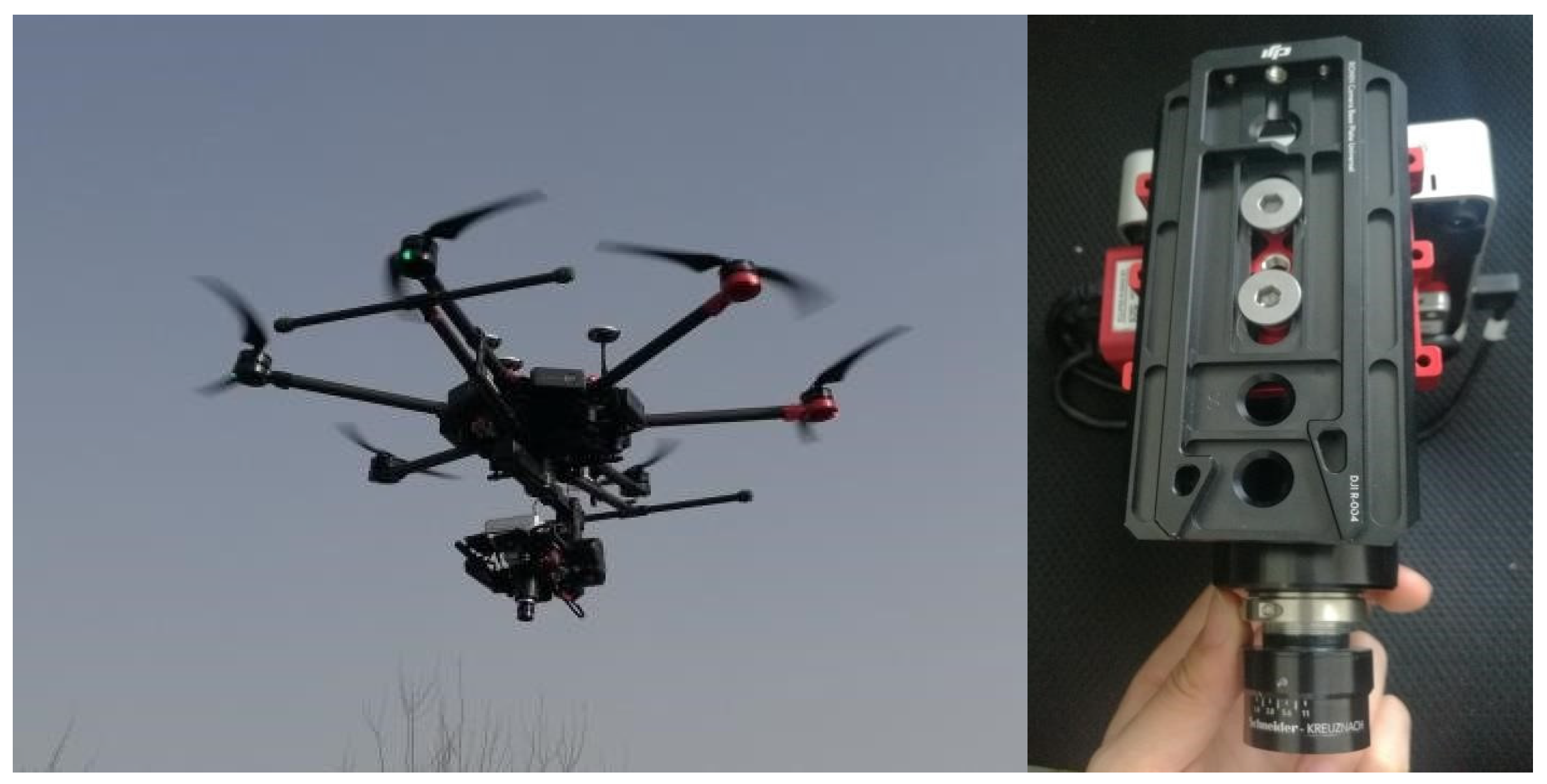
2.2.1. UAV Hyperspectroscopy-Based Image Acquisition

The Resonon-Pika-L airborne imaging spectrometer (Figure 2) from Resonon Company comprises a hyperspectral imaging spectrometer, six-rotor UAV, GPS, and computer. It was used to acquire a hyperspectral image covering the entire study area with a pixel size of 0.05 × 0.05 m on 15 June 2020. The spectra extracted from the hyperspectral image ranged from 400 to 1000 nm, with a spectral resolution of 2.1 nm. Two UAV flight missions were conducted at 11:20 am, with a flight height of 100 m and a speed of 3 m/s. The image field of view (FOV) was 17.6°, and the instantaneous field of view (IFOV) was 0.88 mrad.

2.2.2. UAV Hyperspectral Image Processing

Image Processing

The position and orientation system (POS) data were imported into the SBGcenter software, and geometric correction of each hyperspectral image was performed using the POS post-less differencing technique. Radiation calibration was performed according to the calibration file. After the geographical registration of hyperspectral images along each route in the “Georeferencing” module in ArcGIS 10.2, multiple hyperspectral images of the study area were stitched together in the “map-matching georeferenced” module in ENVI 5.3.

Soil Spectral Extraction

After radiation and geometric corrections, we obtained True Color Images and extracted the spectra of typical objects. Because the UAV image has mixed pixels of vegetation and soil, the difference vegetation index (DVI) was calculated using the ENVI software to differentiate between the two types [22,23]. The average spectral reflectance of the soil pixels (0.05 × 0.05 m) in the range of 1 m² (20 pixels × 20 pixels) was selected as the soil spectrum of a sampling point.

2.2.3. Visible Near-Infrared (NIR) Spectra Acquisition

After the acquisition of the UAV hyperspectral image, visible near-infrared spectra in situ were collected immediately. The spectra were measured using a Quality Spec Trek portable spectrometer (ASD Inc., Boulder, CO, USA) under clear and low-wind weather conditions. The instrument has a spectral range of 350–2500 nm with spectral resolutions of 3 nm at 350–700 nm, 9.8 nm at 700–1400 nm, and 8.1 nm at 1400–2100 nm. The resampling interval was set to 1 nm. At each soil sample point, a whiteboard calibration of the spectrometer was performed before spectrum measurement. The spectrometer probe was oriented vertically downward, and spectral curves were collected from four directions (the angle between adjacent directions was 90°) for each sample point. The in situ spectrum of the soil sample was determined by calculating the average of the four spectra. The spectral collection time was consistent with the soil sample collection time on June 15, 2020. To exclude the effect of spectra larger than the 1000 nm band, we used visible NIR hyperspectral data in the same band range of 420–900 nm as that for UAV.

2.2.4. Spectral Preprocessing

The spectral preprocessing approach may effectively attenuate the spectral noise and minimize the noise generated by background interference from sensors or other devices [24]. Therefore, in this study, the UAV hyperspectral and visible near-infrared spectra were processed by removing the spectrum noise, differentiating the remaining spectral reflectance of bands, and converting them to absorbance. Baseline drift and spectral background noise were then removed using a combination of MSC [25], SG [26], and FD [27] techniques.

2.3. SOM Mapping Using Random Forest (RF) and Hyperspectroscopy Data

RF [25] is an ensemble learning method that has been widely and successfully applied for the prediction and classification of soil characteristics. It generates subsample sets from the training set by bootstrap sampling. Each subsample set was a training set for a tree, and the other data were used to test the model of the tree. The parameters of the model include the maximum number of features used for a node (max_features) and the estimated number of trees (n_estimate). In this study, the random forest regressor package in Python 3.5 was used to construct the RF model. n_estimate was set to a range of 10–500, with an interval of 10, and max_features was set to a range of 1–12, with an interval of 1. The GridSearchCV method in Sklearn was used to obtain the best parameters using the root-mean-square error (RMSE) as the evaluation index. The average predicted SOM value of multiple trees in the RF was used as the final result. In addition, sensitive spectra were obtained by determining the importance of each feature in the RF model.

2.4. Reference DSM Method for Comparison

2.4.1. Semi-Variance Analysis

The geostatistical method [28] uses a semi-variance function to estimate the spatial variability of regionalized variables.

$$\gamma \left(h\right)=\frac{1}{2\times n}\times {\displaystyle \sum }_{k=1}^n{\left[Z\left(x_k\right)-Z\left(x_k+h\right)\right]}^2$$

(1)

where $n$ represents the number of observation pairs that are within the lag distance of $h$; $Z\left(x_k\right)$ and $Z\left(x_k+h\right)$ represent the values of the regionalized variable $Z\left(x\right)$ at locations $x_k$ and $x_k+h$, respectively; $\mathsf{\gamma }\left(h\right)$ represents the semi-variance function value at a distance of $h$ between two points.

The semi-variance function can be fitted using a fitted model (Gaussian, exponential, and spherical). During this process, the parameters mainly include the sill, nugget, range, and partial sill. The sill is the maximum value of the semi-variance function, reflecting the maximum spatial variability of the variable. When the spatial lag distance $h$ is near zero, the semi-variance value is a nugget, which represents the spatial variation on the minimum sampling scale. Strong, moderate, and light spatial autocorrelations are represented by Nugget/Sill values of 0.00–0.25, 0.25, 0.75, and 0.75–1.00, respectively [26]. The range indicates the maximum distance in the spatial correlation.

In this study, GS + 7.0 software was used to obtain the best model of semi-covariance function with the best fitting parameters. To plot the fitted curves and calculate the accuracy of the test set, these parameters were introduced in the PyKrige package in Python 3.7.

2.4.2. OK

The Kriging interpolation obtains the predicted value by weighting the sum of the measured values. Based on an unbiased and optimal estimation, OK considers the sum of the weights of the variables to be one.

$$var\left[Z^{*}\left(x_0\right)-Z\left(x_0\right)\right]=E\left[{\left\{Z^{*}\left(x_0\right)-Z\left(x_0\right)\right\}}^2\right]={\displaystyle \sum }_{n=1}^i{\lambda }_i\gamma \left(x_i,x_0\right)-{\displaystyle \sum }_{n=1}^i{\lambda }_i{\lambda }_j\gamma \left(x_i,x_j\right)$$

(2)

where $Z^{*}\left(x_0\right)$ and $Z\left(x_0\right)$ represent the measured and predicted values, respectively. ${\lambda }_i$ represents the weight of the known point.

Based on the modeling set of samples with intervals of 50 and 100 m, this study determined the semi-covariance function and weights of the known points. The validation position estimates were then computed and compared with the measured values.

2.5. Model Evaluation

In this study, the performance of the models was assessed using R², residual predictive deviation (RPD), and RMSE. The computational formulae for the three indicators are as follows:

$$R^2=\frac{{\left({{\displaystyle \sum }}_{i=1}^n\left(Y_i-\overline{X}\right)\left(X_i-\overline{X}\right)\right)}^2}{{{\displaystyle \sum }}_{i=1}^n{\left(Y_i-\overline{Y}\right)}^2{{\displaystyle \sum }}_{i=1}^n{\left(X_i-\overline{X}\right)}^2}$$

(3)

$$RMSE=\sqrt{\frac{{{\displaystyle \sum }}_{i=1}^n\left(Y_i-X_i\right)}{n}}$$

(4)

$$RPD=\frac{{{\displaystyle \sum }}_{i=1}^n{\left(X_i-\overline{X}\right)}^2}{RMSE}$$

(5)

where $X_i$ represents the observed value, $Y_i$ represents the predicted value, $\overline{X}$ represents the average observation value, $\overline{Y}$ represents the average prediction value, and $n$ represents the sample size.

Large R² and RPD values and small RMSE values indicate a high level of model accuracy. If the RPD is below 1.4, then the model cannot be used for estimation; if it is between 1.4 and 2, then the model may be used for estimation, and it requires improvement; if it is greater than 2, then the model has a great predictive capacity [27].

3. Results

3.1. Basic Statistics

The SOM content in the entire dataset (

Table 1. Descriptive statistics of soil organic matter (SOM) (g kg⁻¹).

Sample Set	N	Mean	Min	Max	SD	CV (%)	Kurtosis	Skewness
The entire dataset	92	18.13	11.95	26.45	2.72	0.15	3.85	0.34
Calibration (50 m)	72	18.12	11.95	26.45	2.86	0.16	0.88	0.5
Calibration (100 m)	20	17.7	12.83	25.82	2.74	0.15	2.98	0.98
Validation	20	18.16	12.59	21.35	2.15	0.12	0.95	−1.06

Note: N is the number of sampling points, CV is the coefficient of variation, and SD is the standard deviation.

) ranged from 12.0 to 26.5 g kg⁻¹ or between 1% and 3%. In the study region, SOM concentration was found to belong to the medium and high levels according to the third national land survey’s cultivated land quality classification (>20 g kg⁻¹ high, 10–20 g kg⁻¹ medium, and <10 g kg⁻¹ low). We found that SOM distribution was close to normal in each dataset. In addition, the variation coefficients (CV) of SOM were all less than one, indicating moderate variation [29].

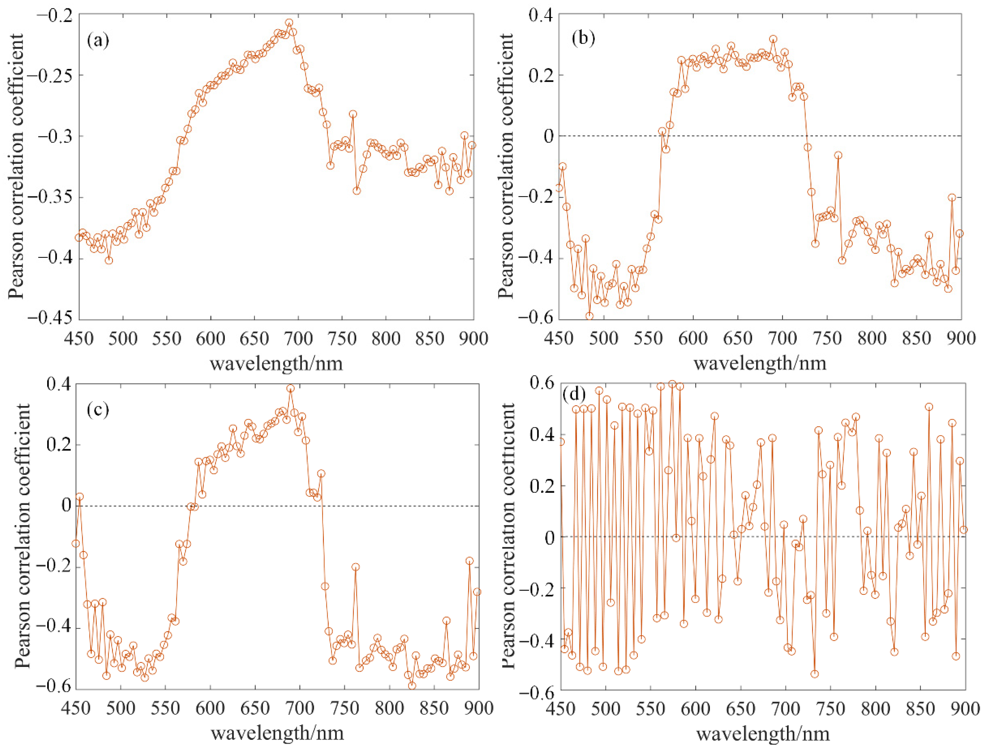
3.2. Spectral Pretreatment Methods for UAV Hyperspectral Data Analysis

The performance of the pretreatment methods was evaluated based on the absolute value of the Pearson correlation coefficient to select the optimal combination of pretreatment methods. As shown in Figure 3, after MSC based on absorbance conversion, the minimum correlation coefficient value changed (−0.4–0.6 at 450–500 nm), the overall correlation coefficient increased at 600–700 nm, the maximum absolute value of the correlation coefficient increased at 700–800 nm, and the correlation coefficient changed (−0.35–0.3 to −0.5–0.3 at 800–900 nm). Overall, MSC amplifies the shape characteristics of the peaks and troughs, expands the range of correlation coefficients, and improves the correlation. Subsequently, after SG, the waveform was essentially unchanged, and the correlation coefficient increased in the 650–700 and 800–900 nm regions. After FD, the curve underwent major changes, with large fluctuations and alternating positive and negative transformations. This is because the original spectral waveform changed significantly after the FD. In summary, the correction between the spectrum and SOM increased after the UAV hyperspectral data were processed by absorbance conversion, MSC, SG (the window size was five and the number of fits was two), and FD, and the strong correlation mainly occurred in the regions of 450–600 nm and 750–900 nm. Subsequently, the spectrum obtained after the combination of these four pretreatment methods was used to construct the model.

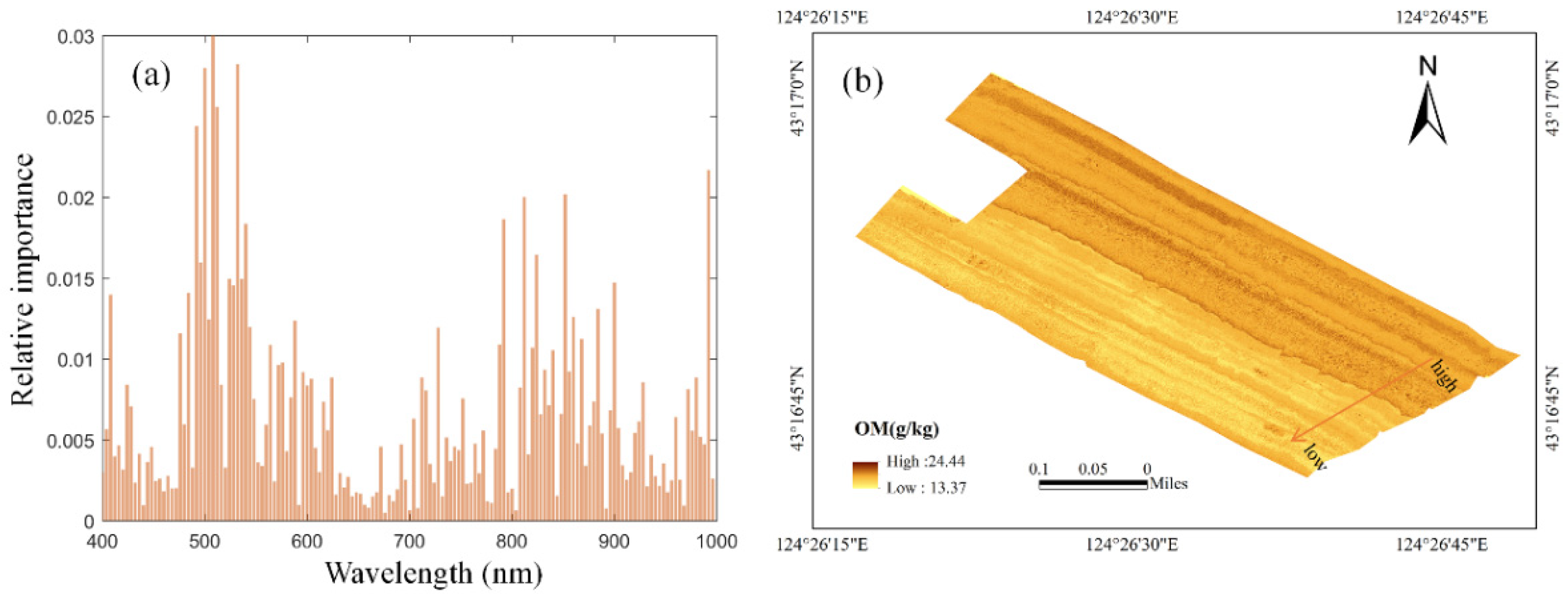
3.3. Performance of the RF Model Using UAV Hyperspectral Data (UAV-RF) in SOM Prediction

Based on the above-mentioned results, the optimal spectral pretreatment method was obtained for RF modeling (R² = 0.53, RMSE = 1.48 g kg⁻¹, and RPD = 1.46) (

Table 2. Performance of the random forest model with UAV hyperspectral data (UAV-RF) on validation data.

Method	Dataset	RMSE (g kg−1)	R2	RPD
UAV-RF	Validation	1.48	0.53	1.46

). This study used the relative importance of the spectrum at each wavelength obtained from the optimal RF model. The results show that 500–550 nm, 730 nm, 790 nm, 800 nm, 850 nm, and 900 nm are the characteristic bands of SOM (Figure 4a). According to the results shown in Section 3.2, the bands with the highest SOM spectrum correlation are located near 522 and 492 nm, which is consistent with the response bands derived using the RF algorithm. This finding confirms that the correlation between the bands and soil properties is related to the importance of these bands in the prediction model. The spatial distribution of SOM (Figure 4b) obtained by RF shows that the SOM values are low in the southwest and high in the north-east, with a highest value of 22.28 g kg⁻¹. In the southeastern part of the study area, some light yellow spots have localized low values; in the northeastern part, most of the high-value spots contain some medium values. Overall, the distribution of SOM was characterized by a patchy and aggregated distribution accompanied by localized maximum values.

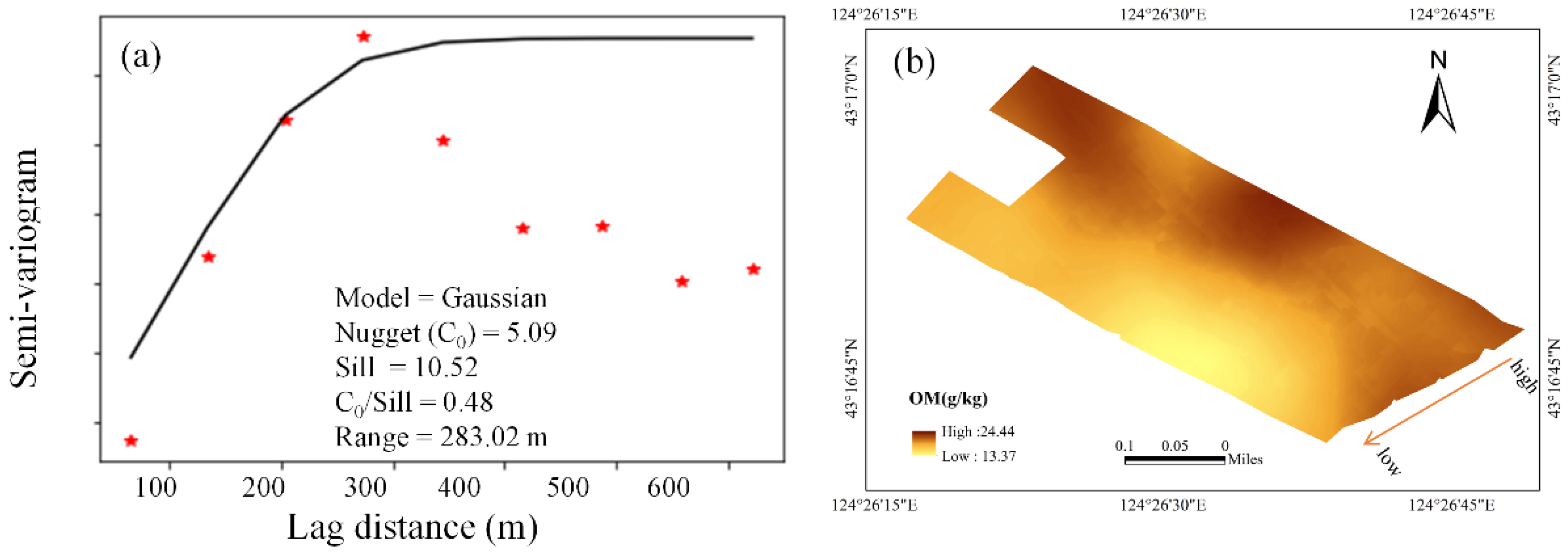
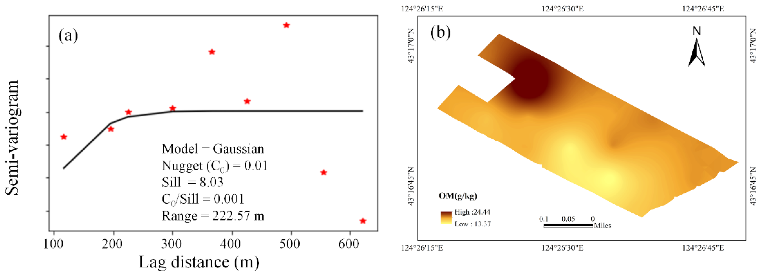
3.4. Performance of OK in SOM Prediction

Using a 100 × 100 m grid sampling strategy, the SOM semi variance function had a poor fit, with an R² of approximately 0.5 (

Table 3. Performance of OK on validation data.

Method	Dataset	RMSE (g kg−1)	R2	RPD
OK (100 m × 100 m)	Validation	2.17	0.02	0.99
OK (50 m × 50 m)	Validation	1.37	0.59	1.57

), due to significant deviation of certain points from the fitted curve. The optimally fitted parameters are shown in Figure 5a—Nugget = 0.01; Sill = 8.03; Range = 222.57 m. Based on these parameters, the study obtained an OK model with R² = 0.02 and RPD = 0.99. Figure 5b shows the SOM spatial distribution obtained using OK. The spatial distribution pattern showed that the high values were mainly located in the north of the study area, and the low values were mainly located in the south-west.

Using the 50 × 50 m grid sampling strategy, the semi-variance function of SOM fitted well, with an R² above 0.8. Only when the lag distance exceeded the range (283.02 m), the semi-variance function of the SOM could not be fitted and had no spatial correlation (Figure 6a). The optimally fitted parameters are shown in Figure 6a: Nugget = 5.09; Sill = 10.52; Range = 283.02 m. Based on these parameters, the study obtained an OK model with R² = 0.59 and RPD = 1.57 (Table 3). The SOM content decreased from the north-east to the south-west, according to the spatial distribution pattern (Figure 6b).

3.5. Performance of the RF Model Using Proximal Sensing (PS-RF) in SOM Prediction

Initially, the study investigated the preprocessing algorithms for visible near-infrared spectroscopy and determined that the optimal preprocessing combination involved removing the spectrum noise, and subsequently converting it to absorbance. The baseline drift and spectral background noise were then removed using a combination of the MSC, SG, and FD techniques. Then, a resampling transformation with a window size of four was used to reduce data redundancy. Finally, a first-order differential was used to amplify the features of the spectrum. A comparison of the data in Table 2 and

Table 4. Performance of the random forest with proximal sensing (PS-RF) on validation data.

Method	Dataset	RMSE (g kg−1)	R2	RPD
PS-RF	Validation	1.41	0.57	1.51

showed that the RMSE (1.48 g kg⁻¹) and R² (0.53) of the UAV-RF were closer to those (RMSE = 1.41 g kg⁻¹; R² = 0.57) of the model based on PS-RF.

4. Discussion

4.1. Spectral Pretreatment Methods

The original spectrum is affected by soil moisture, light, and the instrument itself in the sampling environment; therefore, some details are not obvious or are even disturbed by the noise in the original spectrum. Therefore, it is necessary to use spectral enhancement, denoising, and smoothing techniques to enhance the spectral feature bands. The correlation between the spectrum and soil properties was used as an evaluation index for the spectral prediction model. Previous studies have established that this correlation can determine the characteristic bands of SOM [12]. In the current study, we observed that the absolute value of the correlation coefficient between the spectral transform values and OM increased from 0.41 to 0.58 after absorbance conversion, MSC, SG, and FD processing, which indicates the effectiveness of these four treatments in spectral processing. Consistent with our results, previous studies proposed that logarithmic, first-order differential, MSC, and SG could be effective spectral pretreatments [18,29]. This research provides a spectral pre-processing method for UAV hyperspectral data.

4.2. Characteristic Bands of SOM

The vis-NIR spectra of a material depend on the absorption of light radiation energy by the constituents present in the material; therefore, different substances have various characteristic bands. The results show that 500–600 nm, 730 nm, 790 nm, 800 nm, 850 nm, and 900 nm are the characteristic bands of SOM attributable to the O-H, C-H, and N-H functional groups [30]. Consistent with our results, Lu et al. (2007) discovered that the sensitive band of black soil in north-east China was near 550–830 nm [31] through a correlation analysis between the SOM content and the original spectral reflectance of soil affected by the O-H, C-H, and N-H functional groups; the main response bands of SOM were in the region of 610–2350 nm [32]. This study summarized the characteristic bands of SOM from the previous study findings shown in

Table 5. Soil organic matter (SOM) response bands in previous studies.

Response Bands	References
400–700, 700–2500 nm	[33]
545–738 nm	[31]
450, 700–800, 850–1100 nm	[34]
600–800 nm	[35]
940 nm	[36]
610–2350 nm	[32]

and found that the characteristic bands of SOM vary in the vis-NIR region owing to the influence of the sensors, soil type, water content, and other factors. However, SOM has a strong response characteristic at approximately 700 nm.

4.3. Comparison of the Effectiveness of UAV-RF, PS-RF, and Geostatistical Interpolation for SOM Prediction

Using the 100 × 100 m grid sampling design, the UAV-RF could successfully predict the SOM content, with an R² of 0.53 and RMSE of 1.48 g kg⁻¹, while OK performed poorly, with an R² of 0.02 and RMSE of 2.17 g kg⁻¹. When the number of sampling points was increased to 72 (sampling strategy: 50 × 50 m), OK successfully predicted the SOM with an accuracy comparable to that of UAV-RF with 20 sampling points (R² = 0.59 and RMSE = 1.37 g kg⁻¹). This is because the ability of the semi-variance function to extract SOM spatial variability is enhanced with an increasing sampling density (Figure 5a and Figure 6a), resulting in a substantial increase in prediction accuracy. The geostatistical method is significantly affected by the sampling density [37,38]. When the sampling density is too low, it is difficult to guarantee accuracy. Tsui et al. (2016) analyzed and predicted the spatial variability of soil organic carbon density using four methods—OK, empirical Bayesian kriging (EBK), and inverse distance weighting with four sample subsets (N = 7388, 1168, 370, or 77)—and found that the prediction accuracy decreased with decreasing sampling density [39]. Our findings were similar to those of previous investigations [37,40].

Conversely, the spatial distribution patterns of the SOM generated using the UAV-RF with the 100 × 100 m grid sampling strategy (Figure 4b) and OK with the 50 × 50 m grid sampling strategy (Figure 6b) were generally similar, with the both decreasing from the north-west to the south-east. However, they were different from the spatial distribution patterns obtained from OK with the 100 × 100 m grid sampling strategy (Figure 5b). The high SOM values in the central and southern regions disappeared after reducing the sampling density, which was probably because the information was lost after reducing the sampling points in the central and southern regions of the study area. These findings indicate that the DSM of SOM using OK requires a high sampling density, which causes data redundancy and wastes resources.

Nevertheless, the DSM method based on UAV hyperspectral data using the 100 × 100 m grid sampling strategy can learn the spectral characteristics of SOM through machine learning, which is less affected when it is using the sampling density using grid sampling. In terms of mapping, Figure 4b and Figure 6b show that the SOM content distribution maps based on UAV hyperspectral data contain striped high-value distributions, whereas the interpolated map from OK transitions smoothly. This difference may be because the UAV hyperspectrum provided fine-scale information, and thus reflected more detailed SOM variation. Thus, the UAV hyperspectral data-based DSM provides more detailed information than the interpolation result does.

Using visible and near-infrared (vis–NIR) proximal hyperspectral technology, the prediction results of OM were generally consistent with those of the UAV sensing platform, with RMSE of 1.41 g kg⁻¹ and 1.48 g kg⁻¹ and R² of 0.57 and 0.53, respectively, which indicated that SOM prediction based on the UAV hyperspectral platform was feasible. Additionally, proximal sensing platforms cannot provide continuous spectral features in a specific area. In contrast, UAV hyperspectral technology can acquire dense spectra in a specific area using line array scanning or surface array scanning imaging, which is no longer a single-point-scale manual acquisition method. The acquired UAV hyperspectral images have high-dimensional characteristics, and each image element records spectral information of tens or even hundreds of continuous bands and spatial information simultaneously.

5. Conclusions

This study compared the OK technique for SOM prediction on a field scale using UAV hyperspectral data, observed soil data, and an RF model.

The results were as follows: (1) Absorbance conversion, MSC, SG, and FD techniques were efficient for predicting the SOM. Following these pretreatments, the absolute maximum correlation coefficient between the spectra and SOM increased from 0.41 to 0.58. (2) The characterized bands of the SOM were located at 450–600 nm and 750–900 nm, which might be due to O–H, C–H, and N–H functional group vibrations. (3) Using the 100 m × 100 m grid sampling design, UAV-RF predicted the SOM with an R² of 0.53 and RMSE of 1.48 g kg⁻¹, whereas OK with the same sampling strategy failed to predict the SOM (RMSE = 2.17 g kg⁻¹; R² = 0.02). The poor prediction accuracy was because the low sample density weakened the ability of the semi-covariance function to describe the spatial variability of the SOM. The SOM can be successfully predicted using OK only when the sampling density increases, and the products from OK are comparable to those from UAV-RF. (4) The prediction results of SOM based on the PS-RF were generally consistent with those based on the UAV-RF, yielding RMSE values of 1.41 g kg⁻¹ and 1.48 g kg⁻¹, and R² values of 0.57 and 0.53, respectively. These findings provide a reference for future research and the development of UAV hyperspectral techniques for SOM prediction with a reduced sample size.

References

1. Xu, X.Z.; Xu, Y.; Chen, S.C.; Xu, S.G.; Zhang, H.W. Soil loss and conservation in the black soil region of Northeast China: A retrospective study. Environ. Sci. Policy 2010, 13, 793–800. [Google Scholar] [CrossRef]
2. Rossel, R.V.; McBratney, A.B. Soil chemical analytical accuracy and costs: Implications from precision agriculture. Aust. J. Exp. Agric. 1998, 38, 765–775. [Google Scholar] [CrossRef]
3. Ciais, P.; Gervois, S.; Vuichard, N.; Piao, S.L.; Viovy, N. Effects of land use change and management on the European cropland carbon balance. Glob. Change Biol. 2011, 17, 320–338. [Google Scholar] [CrossRef]
4. Yan, Y.; Kayem, K.; Hao, Y.; Shi, Z.; Zhang, C.; Peng, J.; Liu, W.; Zuo, Q.; Ji, W.; Li, B. Mapping the Levels of Soil Salination and Alkalization by Integrating Machining Learning Methods and Soil-Forming Factors. Remote Sens. 2022, 14, 3020. [Google Scholar] [CrossRef]
5. Zhang, N.; Zhang, X.; Yang, G.; Zhu, C.; Huo, L.; Feng, H. Assessment of defoliation during the Dendrolimus tabulaeformis Tsai et Liu disaster outbreak using UAV-based hyperspectral images. Remote Sens. Environ. 2018, 217, 323–339. [Google Scholar] [CrossRef]
6. Bedini, E.; Van Der Meer, F.; Van Ruitenbeek, F. Use of HyMap imaging spectrometer data to map mineralogy in the Rodalquilar caldera, southeast Spain. Int. J. Remote Sens. 2009, 30, 327–348. [Google Scholar] [CrossRef]
7. Tsouros, D.C.; Bibi, S.; Sarigiannidis, P.G. A review on UAV-based applications for precision agriculture. Information 2019, 10, 349. [Google Scholar] [CrossRef] [Green Version]
8. Adão, T.; Hruška, J.; Pádua, L.; Bessa, J.; Peres, E.; Morais, R.; Sousa, J.J. Hyperspectral imaging: A review on UAV-based sensors, data processing and applications for agriculture and forestry. Remote Sens. 2017, 9, 1110. [Google Scholar] [CrossRef] [Green Version]
9. Recena, R.; Fernández-Cabanás, V.M.; Delgado, A. Soil fertility assessment by Vis-NIR spectroscopy: Predicting soil functioning rather than availability indices. Geoderma 2019, 337, 368–374. [Google Scholar] [CrossRef]
10. Zhu, W.; Rezaei, E.E.; Nouri, H.; Yang, T.; Li, B.; Gong, H.; Lyu, Y.; Peng, J.; Sun, Z. Quick detection of field-scale soil comprehensive attributes via the integration of UAV and sentinel-2B remote sensing data. Remote Sens. 2021, 13, 4716. [Google Scholar] [CrossRef]
11. Hu, J.; Peng, J.; Zhou, Y.; Xu, D.; Zhao, R.; Jiang, Q.; Fu, T.; Wang, F.; Shi, Z. Quantitative estimation of soil salinity using UAV-borne hyperspectral and satellite multispectral images. Remote Sens. 2019, 11, 736. [Google Scholar] [CrossRef] [Green Version]
12. Ivushkin, K.; Bartholomeus, H.; Bregt, A.K.; Pulatov, A.; Franceschini, M.H.; Kramer, H.; van Loo, E.N.; Roman, V.J.; Finkers, R. UAV based soil salinity assessment of cropland. Geoderma 2019, 338, 502–512. [Google Scholar] [CrossRef]
13. Ge, X.; Wang, J.; Ding, J.; Cao, X.; Zhang, Z.; Liu, J.; Li, X. Combining UAV-based hyperspectral imagery and machine learning algorithms for soil moisture content monitoring. PeerJ 2019, 7, e6926. [Google Scholar] [CrossRef] [PubMed]
14. Fang, Y.; Hu, Z.; Xu, L.; Wong, A.; Clausi, D.A. Estimation of iron concentration in soil of a mining area from UAV-based hyperspectral imagery. In Proceedings of the 2019 10th Workshop on Hyperspectral Imaging and Signal Processing: Evolution in Remote Sensing (WHISPERS), Amsterdam, The Netherlands, 24–26 September 2019; pp. 1–5. [Google Scholar]
15. Wei, L.; Zhang, Y.; Lu, Q.; Yuan, Z.; Li, H.; Huang, Q. Estimating the spatial distribution of soil total arsenic in the suspected contaminated area using UAV-Borne hyperspectral imagery and deep learning. Ecol. Indic. 2021, 133, 108384. [Google Scholar] [CrossRef]
16. Geladi, P.; MacDougall, D.; Martens, H. Linearization and scatter-correction for near-infrared reflectance spectra of meat. Appl. Spectrosc. 1985, 39, 491–500. [Google Scholar] [CrossRef]
17. Liu, Y.; Liu, Y.; Chen, Y.; Zhang, Y.; Shi, T.; Wang, J.; Hong, Y.; Fei, T.; Zhang, Y. The influence of spectral pretreatment on the selection of representative calibration samples for soil organic matter estimation using Vis-NIR reflectance spectroscopy. Remote Sens. 2019, 11, 450. [Google Scholar] [CrossRef] [Green Version]
18. Silalahi, D.D.; Midi, H.; Arasan, J.; Mustafa, M.S.; Caliman, J. Robust generalized multiplicative scatter correction algorithm on pretreatment of near infrared spectral data. Vib. Spectrosc. 2018, 97, 55–65. [Google Scholar] [CrossRef]
19. Cheng, H.; Shen, R.; Chen, Y.; Wan, Q.; Shi, T.; Wang, J.; Wan, Y.; Hong, Y.; Li, X. Estimating heavy metal concentrations in suburban soils with reflectance spectroscopy. Geoderma 2019, 336, 59–67. [Google Scholar] [CrossRef]
20. Wollenhaupt, N.C.; Wolkowski, R.P. Grid soil sampling. Better Crops 1994, 78, 6–9. [Google Scholar]
21. Nelson, D.A.; Sommers, L.E. Total carbon, organic carbon, and organic matter. In Methods of Soil Analysis: Part 2 Chemical and Microbiological Properties; Wiley: Hoboken, NJ, USA, 1983; Volume 9, pp. 539–579. [Google Scholar]
22. Tan, C.; Zhang, P.; Zhou, X.; Wang, Z.; Xu, Z.; Mao, W.; Li, W.; Huo, Z.; Guo, W.; Yun, F. Quantitative monitoring of leaf area index in wheat of different plant types by integrating NDVI and Beer-Lambert law. Sci. Rep. 2020, 10, 929. [Google Scholar] [CrossRef] [Green Version]
23. Wagenseil, H.; Samimi, C. Assessing spatio-temporal variations in plant phenology using Fourier analysis on NDVI time series: Results from a dry savannah environment in Namibia. Int. J. Remote Sens. 2006, 27, 3455–3471. [Google Scholar] [CrossRef]
24. Yang, X.; Bao, N.; Li, W.; Liu, S.; Fu, Y.; Mao, Y. Soil nutrient estimation and mapping in farmland based on uav imaging spectrometry. Sensors 2021, 21, 3919. [Google Scholar] [CrossRef] [PubMed]
25. Breiman, L. Random forests. Mach. Learn. 2001, 45, 5–32. [Google Scholar] [CrossRef] [Green Version]
26. Cambardella, C.A.; Moorman, T.B.; Novak, J.M.; Parkin, T.B.; Karlen, D.L.; Turco, R.F.; Konopka, A.E. Field-scale variability of soil properties in central Iowa soils. Soil Sci. Soc. Am. J. 1994, 58, 1501–1511. [Google Scholar] [CrossRef]
27. Chang, C.; Laird, D.A.; Mausbach, M.J.; Hurburgh, C.R. Near-infrared reflectance spectroscopy–principal components regression analyses of soil properties. Soil Sci. Soc. Am. J. 2001, 65, 480–490. [Google Scholar] [CrossRef] [Green Version]
28. Ji, W.; Adamchuk, V.I.; Chen, S.; Su, A.S.M.; Ismail, A.; Gan, Q.; Shi, Z.; Biswas, A. Simultaneous measurement of multiple soil properties through proximal sensor data fusion: A case study. Geoderma 2019, 341, 111–128. [Google Scholar] [CrossRef]
29. Hillel, D. Applications of Soil Physics; Elsevier: Amsterdam, The Netherlands, 2012. [Google Scholar]
30. Stenberg, B.; Rossel, R.V.; Mouazen, A.M.; Wetterlind, J. Advances in Agronomy; Academic Press: Burlington, NJ, USA, 2010; Volume 107, pp. 163–215. [Google Scholar]
31. Lu, Y.; Bai, Y.; Yang, L.; Wang, H. Prediction and validation of soil organic matter content based on hyperspectrum. Sci. Agric. Sin. 2007, 40, 1989–1995. [Google Scholar]
32. Bao, Y.; Meng, X.; Ustin, S.; Wang, X.; Zhang, X.; Liu, H.; Tang, H. Vis-SWIR spectral prediction model for soil organic matter with different grouping strategies. Catena 2020, 195, 104703. [Google Scholar] [CrossRef]
33. Rossel, R.V.; Walvoort, D.; McBratney, A.B.; Janik, L.J.; Skjemstad, J.O. Visible, near infrared, mid infrared or combined diffuse reflectance spectroscopy for simultaneous assessment of various soil properties. Geoderma 2006, 131, 59–75. [Google Scholar] [CrossRef]
34. O’Rourke, S.M.; Holden, N.M. Determination of soil organic matter and carbon fractions in forest top soils using spectral data acquired from visible–near infrared hyperspectral images. Soil Sci. Soc. Am. J. 2012, 76, 586–596. [Google Scholar] [CrossRef]
35. Ji, W.; Shi, Z.; Zhou, Q.; Zhou, L. VIS-NIR reflectance spectroscopy of the organic matter in several types of soils. J. Infrared Millim. Wave 2012, 31, 277–282. [Google Scholar] [CrossRef]
36. Kweon, G.; Maxton, C. Soil organic matter sensing with an on-the-go optical sensor. Biosyst. Eng. 2013, 115, 66–81. [Google Scholar] [CrossRef]
37. Zhang, Z.; Yu, D.; Shi, X.; Wang, N.; Zhang, G. Priority selection rating of sampling density and interpolation method for detecting the spatial variability of soil organic carbon in China. Environ. Earth Sci. 2015, 73, 2287–2297. [Google Scholar] [CrossRef]
38. Njoku, E.A.; Akpan, P.E.; Effiong, A.E.; Babatunde, I.O. The effects of station density in geostatistical prediction of air temperatures in Sweden: A comparison of two interpolation techniques. Resour. Environ. Sustain. 2023, 11, 100092. [Google Scholar] [CrossRef]
39. Tsui, C.; Liu, X.; Guo, H.; Chen, Z. Effect of Sampling Density on Estimation of Regional Soil Organic Carbon Stock for Rural Soils in Taiwan. In Geospatial Technology-Environmental and Social Applications; InTech: Rijeka, Croatia, 2016; pp. 35–53. [Google Scholar]
40. Sun, W.; Zhao, Y.; Huang, B.; Shi, X.; Landon Darilek, J.; Yang, J.; Wang, Z.; Zhang, B. Effect of sampling density on regional soil organic carbon estimation for cultivated soils. J. Plant Nutr. Soil Sci. 2012, 175, 671–680. [Google Scholar] [CrossRef]
Figure 1. Soil sample distribution in the study area.
Remotesensing 15 01433 g001
Figure 2. Resonon-Pika-L airborne imaging spectrometer.
Remotesensing 15 01433 g002
Figure 3. Correlation coefficients between soil organic matter (SOM) and soil spectral characteristics after (a) absorbance conversion, (b) multiplicative scatter correction, (c) Savitzky–Golay (the window size is 5, and the number of fits is 2), and (d) first derivative methods.
Remotesensing 15 01433 g003
Figure 4. Importance analysis (a) and map (b) of the RF model using UAV hyperspectral (UAV-RF) in soil organic matter (SOM) prediction.
Remotesensing 15 01433 g004
Figure 5. Semi-variance function (a) and map (b) of ordinary kriging (OK) in SOM prediction using a 100 × 100 m grid sampling strategy.
Remotesensing 15 01433 g005
Figure 6. Semi-variance function (a) and map (b) of ordinary kriging (OK) in SOM prediction using the 50 × 50 m grid sampling strategy.
Remotesensing 15 01433 g006