Article

Hyperspectral Anomaly Detection with Differential Attribute Profiles and Genetic Algorithms

1
Key Laboratory of Airborne Optical Imaging and Measurement, Changchun Institute of Optics, Fine Mechanics and Physics, Chinese Academy of Sciences, Changchun 130033, China
2
University of Chinese Academy of Sciences, Beijing 100049, China
3
Changchun Institute of Optics, Fine Mechanics and Physics, Chinese Academy of Sciences, Changchun 130033, China
*
Author to whom correspondence should be addressed.
Remote Sens. 2023, 15(4), 1050; https://doi.org/10.3390/rs15041050
Submission received: 5 January 2023 / Revised: 3 February 2023 / Accepted: 11 February 2023 / Published: 15 February 2023
(This article belongs to the Special Issue Advances in Hyperspectral Remote Sensing Image Processing)

Abstract

:
Anomaly detection is hampered by band redundancy and the restricted reconstruction ability of spectral–spatial information in hyperspectral remote sensing. A novel hyperspectral anomaly detection method integrating differential attribute profiles and genetic algorithms (DAPGA) is proposed to sufficiently extract the spectral–spatial features and automatically optimize the selection of the optimal features. First, a band selection method with cross-subspace combination is employed to decrease the spectral dimension and choose representative bands with rich information and weak correlation. Then, the differentials of attribute profiles are calculated by four attribute types and various filter parameters for multi-scale and multi-type spectral–spatial feature decomposition. Finally, the ideal discriminative characteristics are reserved and incorporated with genetic algorithms to cluster each differential attribute profile by dissimilarity assessment. Experiments run on a variety of genuine hyperspectral datasets including airport, beach, urban, and park scenes show that the effectiveness of the proposed algorithm has great improvement with existing state-of-the-art algorithms.

1. Introduction

With narrow spectral intervals and contiguous spectral ranges, hyperspectral imagery is a three-dimensional image cube that contains a wealth of spatial characteristics and uniquely diagnostic spectral signatures to distinguish different materials. The remarkable discriminability of HSI has been used in a variety of missions, including spectral unmixing, scene classification, and target detection [1,2,3]. Anomaly detection is regarded as an unsupervised binary classification to separate unusual objects that have distinct spectral or spatial differences from their surroundings. Nowadays, hyperspectral anomaly detection has become a frontier and promising technology for remote sensing applications [4,5].
The first and most prevalent category is the statistical model-based technique in hyperspectral detection. The famous Reed–Xiaoli (RX) method [6] is dependent on the presumption that the background obeys a multivariate Gaussian distribution so that the background can be described using the mean vector and the covariance matrix of the pixels. The Mahalanobis distance between the spectral vectors of a test pixel and its surroundings is the outcome of the resulting generalized likelihood ratio test. Its extensions, called Local RX (LRX) [7] and Global RX (GRX) [8], use predefined local windows around test pixels and the entire image, respectively, to estimate background statistics. However, in some certain real scenes, the homogeneous distribution is too simple to describe the majority of HSIs that span different materials with complicated backgrounds. Moreover, due to the existence of noisy and other anomalous pixels, the mean vector and the covariance matrix are inaccurate for background description. To address these limitations, there have been various improved algorithms, such as the kernel RX algorithm [9], the selective Kernel PCA and RXD [10], the weighted-RXD and linear filter-based-RXD [11] and robust nonlinear learning-based detection method [12], which typically produce excellent detection results. Lately, the fractional Fourier transform has been included in the preprocessing step of the fractional Fourier entropy and RX hyperspectral anomaly detection (FrFE-RX) [13] to significantly distinguish the signal from background and noise. Although it performs better than RX, it also requires more running time. Even though it performs better than RX, extra running time is also required.
Due to background distribution assumptions not being necessary, geometrical modeling-based methods have attracted widespread attention. Collaborative representation, sparse representation and tensor representation detectors have been the subject of extensive research. They suppose that whereas anomalies cannot be roughly constructed from a collection of major spectra or bases retrieved from the HSI, background pixels may. The discrepancy between a test pixel and its neighbors is captured by the collaborative representation-based detector (CRD) [14], as well as the l2-norm minimization of the representation weight vector strengthens the collaboration of representation. The recursive CRD (RCRD) [15] and the relaxed CRD [16] modify the CRD model to facilitate computational efficiency and improve the robustness of the algorithm, respectively. A counterpart of CRD is sparse representation-based detector (SRD) [17], where l1-norm minimization is employed to solve sparse representation coefficients. The issue that l1-norm minimization does not always produce a suitably sparse solution when a dictionary is not wide enough or atoms exhibit a certain degree of coherence is resolved by adaptive iterated shrinkage thresholding-based lp-norm sparse representation [18]. The low-rank representation detectors [19] or sparse decomposition detectors [20,21] explore the low-rank prior background knowledge to identify sparse pixel locations. The hyperspectral data are divided into a third-order tensor by the tensor representation detector [22], which is made up of a core tensor and three-factor matrices, and the three-factor matrices correspond to the background and abnormal information. The surrounding pixels may still include target pixels even when the representation-based detectors did not take the hypothesis of background distribution into account. It will impede representation outcomes and cause omitted detections.
Some powerful classification tools commonly employed in image processing have been utilized to detect hyperspectral anomalies, for instance, the support vector data description (SVDD) [23], kernel isolation forest-based detector (KIFD) [24,25] and deep learning-based detector [26], which can effectively separate targets from the background. In detail, the SVDD-based detector incorporates a nonparametric background model obeyed the hypothesis that a linear combination with adjacent pixels could stand for the background but it cannot depict the anomalies. The kernel isolation forest-based detector constructs an isolation forest (iForest) following a supposition that anomalies may be more vulnerable to isolation in the kernel space than in the background. Furthermore, the deep learning architecture with stacked autoencoders (SAE) [27], deep belief network [28], convolutional neural network (CNN) [29,30] and autoencoding adversarial network (AEAN) [31] extract high-level distinctive spectral–spatial features in an unsupervised manner. An unsupervised neural network framework with spectral mapping and feature selection (SMFS) [32] is designed to establish the nonlinear mapping relationship from high-dimensional spectral space to low-dimensional deep feature space for describing the fundamental hyperspectral characteristics. For exploiting the spatial correlation of representation coefficients, a convolutional neural network denoiser is plugged into a plug-and-play framework to compose the DeCNN-AD method [33], which could carefully exclude anomalous pixels and include background pixels from clustering results. An autonomous hyperspectral anomaly detection network (Auto-AD) [34] rebuilds the anomalous pixels that present through reestablishing errors. Although existing deep learning-based and other anomaly detectors are useful for hyperspectral anomaly detection, they need to set the parameters manually, increasing the computational complexity.
Another type of detection method has recently achieved compelling performance by exploring spectral–spatial information in HSIs. Mathematical morphological profiles (MPs) [35,36] and attribute profiles (APs) [37,38,39] have proved to be useful means to analyze the spatial domain of images. Moreover, the extinction profiles (EP) [40] and extended morphological profiles (EMP) [41,42] have also been successfully extended to hyperspectral images. Attribute and edge-preserving filters detector (AED) [43] is one of these strategies that was first presented by Kang. It uses attribute filters to extract anomalies by specific area properties and unique spectral characteristics, and the edge-preserving filter for post-processing smooths the outcomes. The multi-scale features were taken into account by developing a multi-scale AED [44]. The current detectors with attribute profiles have demonstrated their capability for hyperspectral anomaly detection. Nevertheless, they still suffer from some problems. Choosing the “significant” filtering parameters from the profiles is an essential procedure for achieving high detection accuracy that only relies on manual tuning or empiricism, which is one limitation in real applications. Although attribute profiles can be used to extract spatial contextual features in the surrounding pixels, they are not good at differentiating the target from the background. Additionally, a complete reconstruction of spatial characteristics cannot be achieved when only one fixed type of attribute is employed to represent the spatial features.
To deal with the aforementioned issues, a novel anomaly detection method based on differential attribute profiles and genetic algorithms is proposed. The innovative contributions can be summarized as follows.
(1)
A novel coarse-to-fine framework is presented integrating the cross-subspace combination band selection, differential attribute profiles, and genetic algorithms for optimal spectral–spatial features’ automatic selection and joint detection.
(2)
A differential algorithm and threshold selection criteria are proposed for the four attribute descriptors to effectively protrude the anomaly objects and adapt to the detection of various size targets in the HSIs.
(3)
An intelligent optimization strategy via genetic algorithms and clustering method is designed, which selectively retain optimal profiles and guarantee a good tradeoff between the representable power of differential attribute profiles and their redundancy.
The paper is organized as follows. Some related concepts of the attribute profile and genetic algorithms are reviewed in Section 2. In Section 3, the proposed method with differential attribute profiles and genetic algorithms (DAPGA) is introduced. The results of real hyperspectral dataset experiments are given in Section 4. The DAPGA method is discussed in Section 5. Finally, a conclusion is presented in Section 6.

2. Related Work

The related concepts and theories about the attribute profiles (APs) and genetic algorithms (GAs) are given in this section. By maintaining or eliminating the connecting components in conformity with preset attribute predicates, the APs can efficiently capture the spatial constructions in the HSIs. Additionally, the selection of reasonable filter parameters is good for improving the discriminative power and avoiding information redundancy, so genetic algorithms are employed to automatically choose optimal features that are independent and representative. The following subsections provide more details about the APs and GAs.

2.1. Attribute Profile

The attribute profile is a multi-level morphological decomposition method using attribute filters (AFs) [45]. In comparison to conventional morphological filters, attribute filters based on geodesic reconstruction are particularly advantageous in terms of computational complexity and capabilities in characterizing the objects in the HSIs. The faster implementation relies on an efficient data structure called max-tree, which is a hierarchical tree that can completely represent a grayscale image. Unlike typical image filtering processes, which are carried out directly at the pixel level, AFs operate at the level of connected components (CC). In other words, an AF is applied on the tree’s node level with regard to a specific attribute predicate.
A sequence of AFs extracts the spatial information by contextual image transformation, which reduces scene complexity and attenuates the insignificant details by integrating the flat regions and not distorting the edges of the regions. Different parametric features can be modeled according to the types of attributes considered in the transformation. The structuring element (SE) is employed in the sliding window of geometrical characteristic extraction, which determines the processing degree for the HSIs. According to the predefined attribute predicate T and threshold λ, SE operates on the pixel values and takes the surrounding pixels into account. The threshold decomposition principle [46] decomposes the input image into a series of binary images, and the upper- and lower-level sets E are yielded by different filtering effects (e.g., T λ ( C C ) > λ and T λ ( C C ) < λ ). A sequence of thickening operations based on a min-tree { ϕ } λ 1 λ N and thinning operations based on a max-tree { γ } λ 1 λ N are performed by integrating the surrounding of an upper and a lower gray level ( C C E ), respectively. Therefore, the thinning operator reacts on the brighter objects in comparison to the adjacent region, and the thickening reacts on darker objects. The attribute profiles acquired by a grayscale image f ( f : 2 ) can be formalized by:
A P f = ϕ λ N ( f ) , ϕ λ N 1 ( f ) , , ϕ λ 1 ( f ) , f , γ λ 1 ( f ) , , γ λ N 1 ( f ) , γ λ N ( f )
In fact, many different AFs are formulated by the logical predicate, including the purely geometric descriptors (e.g., area, moment of inertia, diagonal length of bounding box) and the textural descriptors (e.g., standard deviation, entropy). To properly incorporate spatial features, it could be beneficial to utilize multiple attribute descriptors to extract various target spatial characteristics. Due to the advantages of multi-level spatial construction description and low computational load, the attribute profile is applied to extract the multi-scale and multi-type features of anomaly targets.

2.2. Genetic Algorithms

Genetic algorithms [47] are widely employed for finding solutions to optimization problems on the foundation of natural selection and chromosomal evolutionary processes, which possess the characteristics of parallelism, efficiency and robustness. GAs transform each feasible solution of the desired problem into an individual in biological evolution, search for the stronger environmentally adaptive genetic traits for selective reservation generation by generation, and gradually increase their number in the population, finally finding the globally optimal solution. The desired objective function does not need to satisfy the derivative or continuity conditions. The definition domain of GAs can be set arbitrarily by implementing coding, and the convergence of the algorithm to the optimal solution is independent of the initial population selection. In order to select the representative and informative attribute profiles to describe features, GAs have been introduced for hyperspectral anomaly detection. A collection of chromosomes defined as the population stands for one potential combination mode of the optimal attribute profiles.
Initializing the population is the first step of genetic algorithms to randomly generate chromosomes, and the fitness evaluation assesses each population member. After that the selection, crossover and mutation steps are operated by modifying or recombining the chromosome to produce a new population. The above steps are repeated until the convergence is achieved. The details of GAs used in this paper are given below:
Fitness evaluation: One of the most crucial components of genetic algorithms is the calculation of the fitness value of each chromosome in the population. Fitness evaluation can evaluate the adaptive capacity of every chromosome. In this paper, the fitness function F is exploited to estimate the dissimilarity of attribute filtered images.
Selection: The chromosomes with high fitness values are preserved and retained in the next generation after the fitness evaluation. The fresh individuals generated by crossover and mutation operations would replace all other chromosomes. The most basic and common method of selection is the fitness scale method, where the probability P i of ith individual being selected is proportional to the fitness value F i :
P i = F i i = 1 N F i
Crossover: The child chromosomes in the new generation are produced based on the information exchange that they receive the chromosome segments from their parents. The crossover factor indicates the probability of crossover occurrence. In this way, if some children could inherit superior genes from both parents, they will exceed the performance of their parents.
Mutation: To avoid the likelihood of achieving local maxima, a mutation operation similar to the natural evolutionary process is employed. Bits of a chromosome are probably to be reversed after the crossover operation, which increases the diversity of the population.

3. Materials and Methods

The proposed DAPGA method is presented at a detailed level, and the schematic diagram is depicted in Figure 1. The initialization step is the band selection aiming to reduce the curse of the dimensionality problem and pick typical bands with sufficient information and weak correlation. Subsequently, differential attribute profiles (DAPs) are obtained with attribute filtering and differential operation for multi-scale and multi-type spectral–spatial feature extraction. Furthermore, genetic algorithms are employed to cluster each differential attribute profile by calculating the dissimilarity and obtain a certain number of cluster centers as the optimal DAPs. Finally, these optimal DAPs are fused to generate a final detection map by thresholding and weighted average. The typical band number, the threshold number of each attribute and the cluster centers’ number are represented by b, m and n, respectively. The following subsections provide a detailed explanation of each process.

3.1. Cross-Subspace Combination Band Selection

The spectrometer generally has a higher spectral resolution, so the differences between contiguous spectra are usually small. To reduce the redundancy, the algorithm for band selection primarily evaluates two factors: informative and less correlation between the picked bands. A correlation coefficient R is employed as a reference to calculate the correlation values between each band in the HSI. The correlation coefficient R is calculated as follows:
R = x = 1 M y = 1 N ( f ( x , y ) f ¯ ) × ( g ( x , y ) g ¯ ) x = 1 M y = 1 N ( f ( x , y ) f ¯ ) 2 x = 1 M y = 1 N ( g ( x , y ) g ¯ ) 2
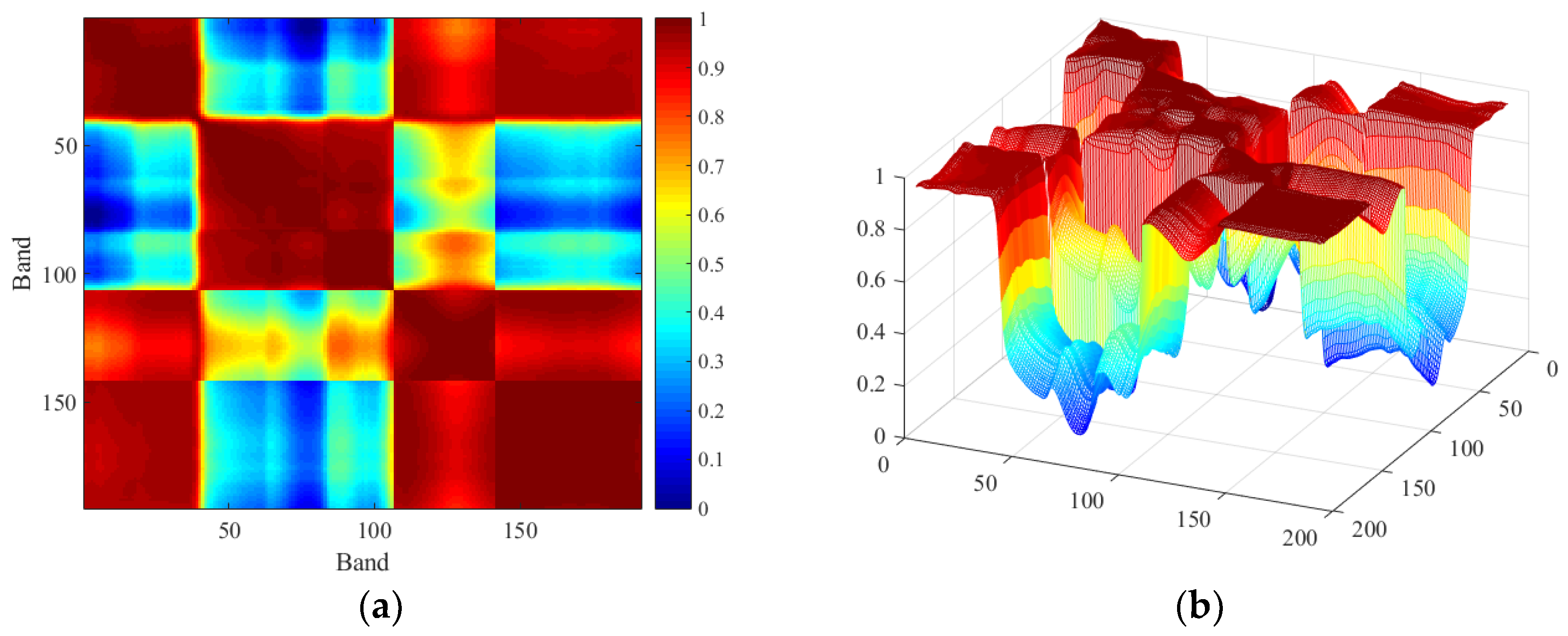
As mentioned, the gray image values of two different bands are expressed as f (x, y) and g (x, y). The average gray values are f and g ¯ . The hyperspectral dataset of the Gulfport airport scene acquired by the Airborne Visible Infrared Imaging Spectrometer (AVIRIS) is availed of to analyze the results of the correlation coefficient matrix, which are displayed in Figure 2. The dataset’s band order is exhibited on the coordinate axis, which comprises 191 effective bands after removing some bands with lower SNR and water absorption. The correlation coefficient values near the diagonal are larger than the others and close to 1. It is clear that the red block effect close to the diagonal indicates that the dataset could be divided into three subspaces according to the correlation degree distinguished by different colors. Moreover, more subspaces can be obtained by averaging each previous subspace.
The optimum index factor (OIF) is exploited for measuring the overall amount of information and the independence with its adjacent bands. The OIF of each band in the same subspace is calculated together, and the band with the maximum value of OIF is selected as the optimum band to represent this subspace. Equations (4) and (5) are the mathematical formulations of OIF.
O I F i = σ i ( R i 1 , i + R i , i + 1 ) / 2
σ i = x = 1 M y = 1 N ( f i ( x , y ) f i ¯ ) 2 M × N
where σi is the standard deviation of band i, and Ri, i+1 denotes the correlation coefficient between the band i and band i + 1. When the correlation declines, the independence between two contiguous bands grows. The pixel size of rows and columns are expressed as M and N in the hyperspectral image, respectively. The bands with the higher image entropy are extracted as the best bands to represent the HSIs when the subspace number surpasses the desired band number.

3.2. Feature Extraction with Differential Attribute Profiles

Four attribute descriptors including area, diagonal length of the box bounding the region, moment of inertia and standard deviation are picked up to generate more characterizations of spatial structures. The different thresholds are designed to identify anomalies of various sizes that are usually small and have a low proportion of pixels in the HSIs. Moreover, the differential operation of four attribute profiles enlarges the details that are different from the background. The differences between attribute filtered images of the area and the diagonal length are computed by the differential operation:
A i = | ϕ A ( f i ) f i | + | f i γ A ( f i ) | = ϕ A ( f i ) γ A ( f i )
L i = | ϕ L ( f i ) f i | + | f i γ L ( f i ) | = ϕ L ( f i ) γ L ( f i )
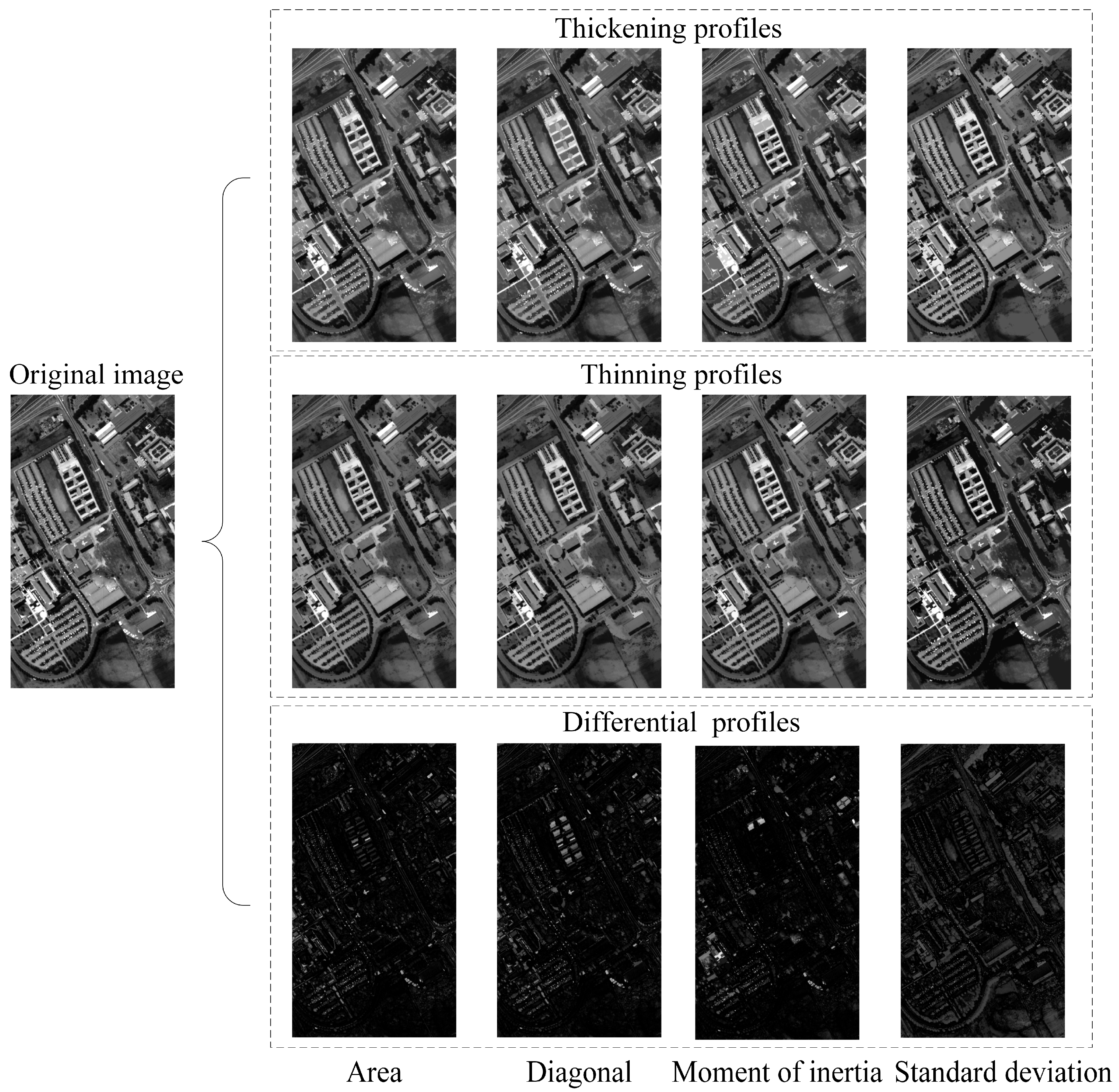
where ϕ and γ stand for thickening and thinning operation, respectively. Ai is the ith area differential map (e.g., see Figure 3), which refers to the probabilities of dark objects | ϕ A ( f i ) f i | and bright objects | f i γ A ( f i ) | in the ith typical band. Since ϕ A ( f i ) f i and f i γ A ( f i ) are always satisfied for each image pixel, the original image can be removed, and thus the area differential map can be directly calculated as ϕ A ( f i ) γ A ( f i ) . Regarding the area attribute, the thresholds τ A are selected by taking into account the resolution ρ and the size M × N of the image, and they are summarized and manifested in the following equation.
τ A = a min 2 , ( a min + δ A ) 2 , ( a min + 2 δ A ) 2 , , a max 2
where the upper and inner bounds are marked as a max and a min , respectively; a min = 3 and a max < 3 × min ( M , N ) / ρ a max 19 , and the step size increase δA is 1. The reasonable threshold range of the diagonal length is also chosen according to the resolution ρ and the size M × N of the image:
τ L = l min , l min + δ L , l min + 2 δ L , , l max
The step increase δL of 2 with l min = 5 and l max < 3 × a max . Therefore, the area and diagonal length could complement each other.
The differential operation of standard deviation and moment of inertia are employed to compute the differences between the attribute filtered images and the original image.
S i = ϕ s ( f i ) f i | | f i γ s ( f i )
I i = ϕ I ( f i ) f i | | f i γ I ( f i )
where Si is the ith standard deviation differential map and Ii is the ith moment of inertia differential map. The reference thresholds of the standard deviation differential map are set based on the whole hyperspectral image’s mean and are covered the reasonable range of deviation.
τ S = δ min , δ min + δ S , δ min + 2 δ S , , δ max
The bottom and top limitation of δ are 5% and 25% of the mean, respectively, and the step increase δS is 2.5% of the mean. Additionally, the reference thresholds of the moment of inertia are set from 0.1 to 0.9, and the interval is 0.1. After the differential operation, all of the differential attribute profiles should be normalized.
The examples in Figure 3 depict four types of attribute profiles that were computed on one typical band of the Pavia university dataset. The attribute profiles created by various attribute descriptors are displayed in each column. The attributes include area, diagonal length, moment of inertia, and standard deviation, starting from the first column. Each attribute comprises three levels that are thickening profile, thinning profile and differential profile. All the transformations are computed with the following attribute thresholds: area: 100; diagonal length: 25; moment of inertia: 0.4; standard deviation: 30.
The figure indicates how one typical band image is processed by the thickening, thinning, and differential transformations by different attribute descriptors. Although the area, diagonal length and moment of inertia all belong to purely geometric descriptors, they perform differently in certain details. The area attribute extracts both dark and bright connected regions to retain the anomaly targets with areas less than the area threshold. The diagonal length attribute also retains objects with diagonal lengths smaller than the diagonal threshold. For the moment of inertia, the elongated structures and the small homogeneous targets are revealed clearly. Furthermore, a few tiny areas of high contrast are retained in the standard deviation attribute profile which may be lost in other attributes.

3.3. Optimal Differential Attribute Profile Selection and Fusion

Large numbers of differential attribute profiles provide abundant spatial information but also lead to the accumulation of redundant features. To mitigate this problem, an optimization step is designed to select a representative subset of DAPs by an unsupervised approach. In combination with the normalized mutual information (NMI) and clustering algorithm, GA is explored to pick up a subgroup of independent and representative DAPs as the optimal features.
NMI is commonly designed to assess the similarity degree among pairs of attribute filtered images. The correlation of NMI for two images fi and fj is calculated as:
N M I ( f i , f j ) = 2 M I ( f i , f j ) H ( f i ) + H ( f j ) = 2 g x G i g y G j p ( g x , g y ) log ( p ( g x , g y ) p ( g x ) p ( g y ) ) g x G i p ( g x ) log ( p ( g x ) ) + g y G j p ( g y ) log ( p ( g y ) )
where MI is the mutual information between two images, and H stands for the image entropy. Gi and Gj are the set of distinct gray values. p(gx, gy) represents the joint probability mass function. As a consequence, the dissimilarity [48] expressed by NMI can be explained as:
D N M I = ( 1 N M I ( f i , f j ) ) 2
The clustering algorithm is employed to classify all the normalized differential attribute profiles according to the artificially set number of clustering centers. The clustering principle is the differential attribute profile is representative as well as acquires a higher dissimilarity value with other cluster representatives. The clustering algorithm is used as the fitness function of GA to compute the dissimilarity ratio of intra-cluster to inter-cluster, and the lower ratio represents the better clustering effect. Let 1, 2, …, q be the cluster index and the differential attribute profiles of cluster centers are fc1, fc2, …, fcn, so Cci represents the number of images belonging to cluster ci as well as fj is the intra-cluster member. The chromosomes are composed of real number encoding, expressing the index of differential attribute profiles, with a reasonable range from 1 to the total number q of profiles. Specifically, the size of the chromosome is the same as the clustering center number n. The fitness function of the genetic algorithms is expressed as:
F = 1 n i = 1 n 1 C c i f j C c i D N M I ( f c i , f j ) 1 n 1 i = 1 n min j i j 1 , 2 , , n D N M I ( f c i , f c j )
After the GA converges to a stable situation, thresholding operations are performed on the optimal differential attribute profiles to generate a collection of Boolean maps B and it could further penalize background information in large regions
B = T h r e s h f ,   θ
where θ is the image threshold, which is determined by Otsu’s approach because of its robustness. Finally, the optimal differential attribute profiles are fused based on the weighted average of its intra-cluster number Cci to form the final detection map. Moreover, x and y stand for the pixel coordinate position:
d D A P G A ( x , y ) = 1 q i = 1 n C c i B c i ( x , y )

4. Results

4.1. Hyperspectral DataSets

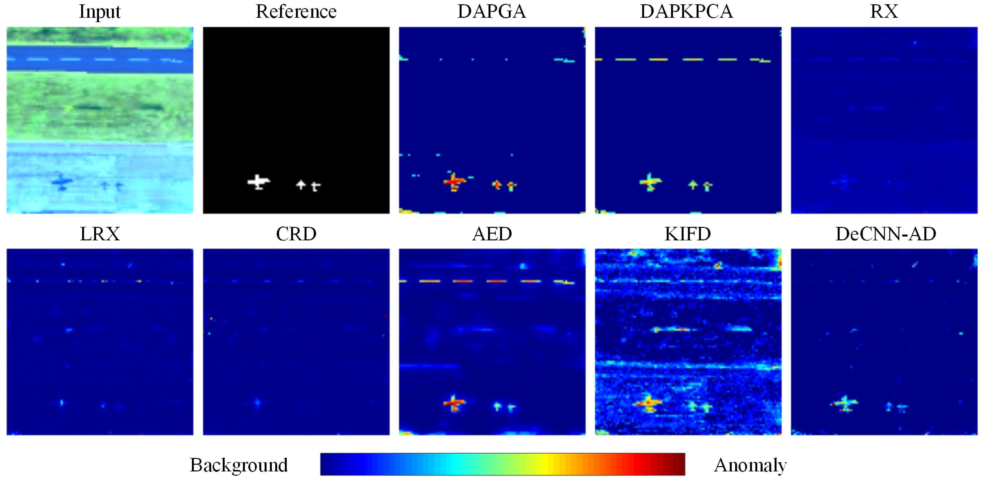
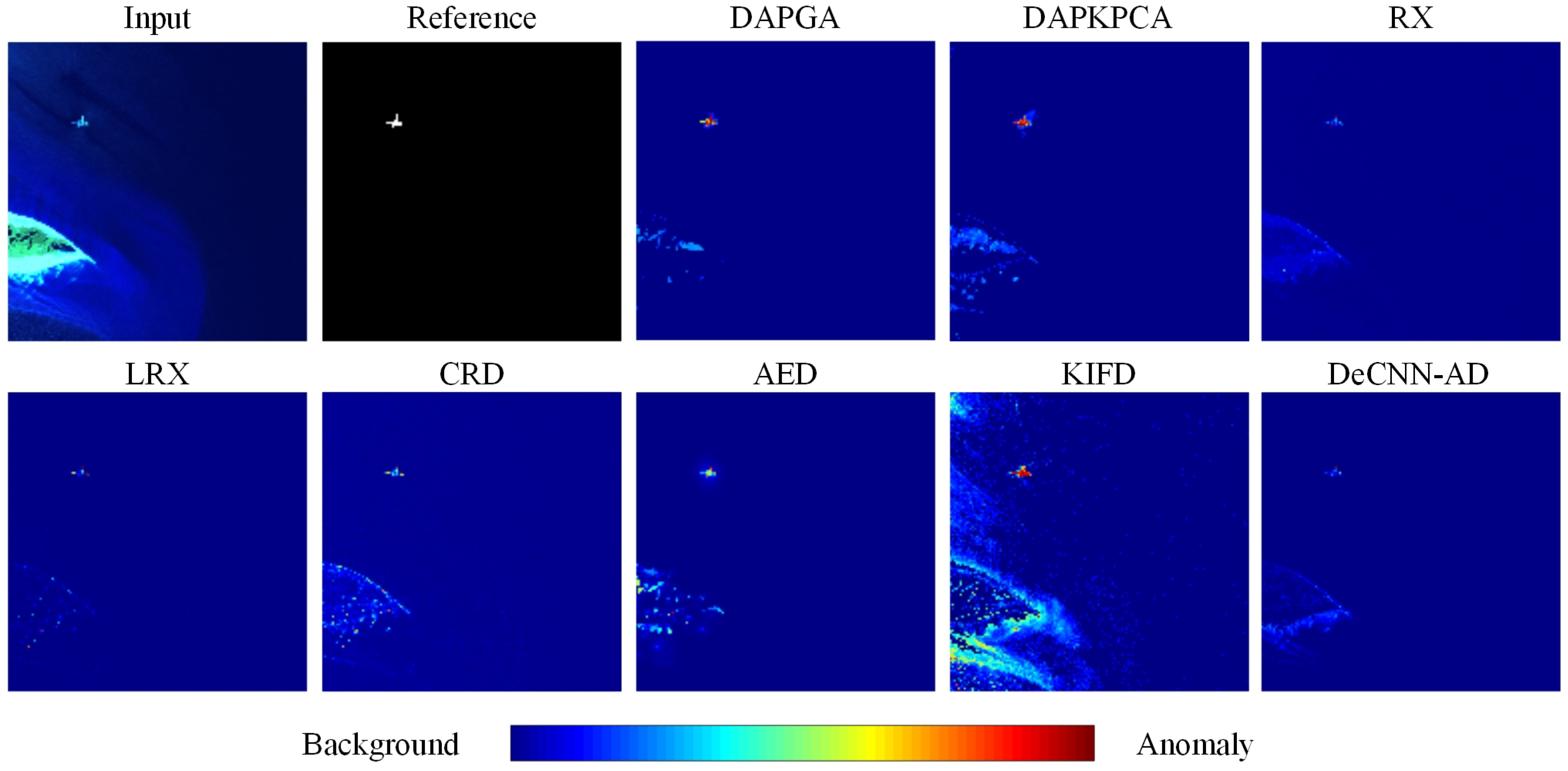
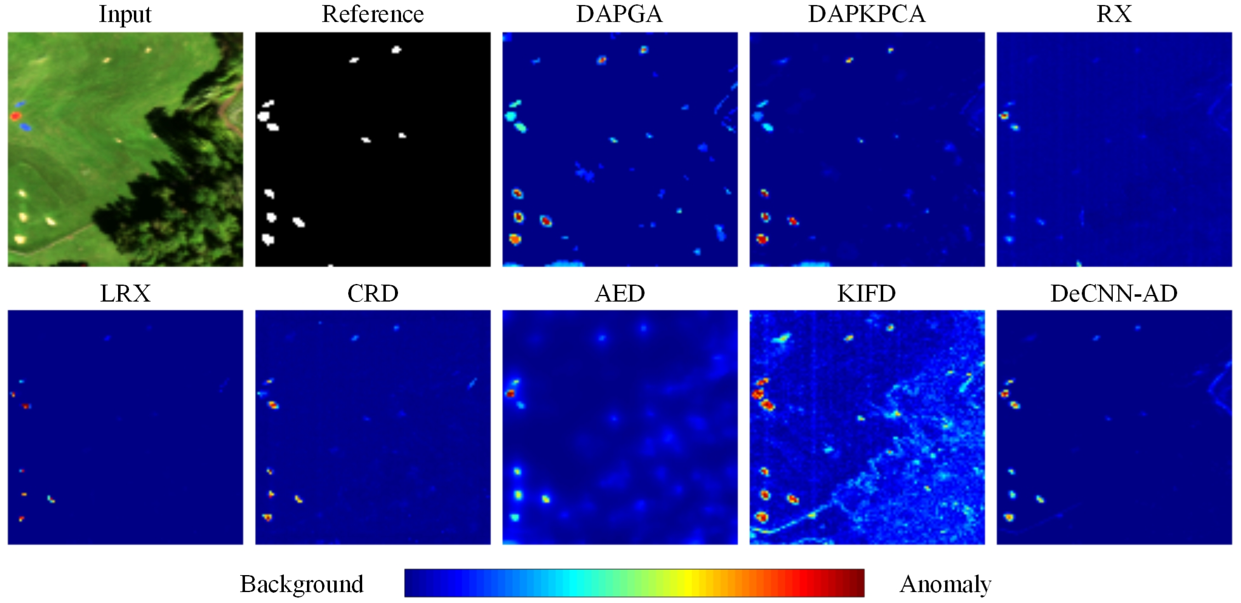
Four real hyperspectral datasets were applied in the experiments to test the proposed method in various scenarios including with targets of different sizes, shapes and materials. The input pseudocolor image and reference ground-truth map for each dataset are presented in Figure 4, Figure 5, Figure 6 and Figure 7. Some features of the four datasets are recorded in Table 1.
(1)
Gulfport Airport Dataset: This hyperspectral dataset was obtained by the AVIRIS sensor in the Gulfport airport, CA, USA. The airport landscape contains an airport runway, tarmac and greenery, and has 100 × 100 pixels with a wavelength range of 400–2500 nm. After the removal of more severe moisture and noisy bands, 191 bands are retained in the experiments. The anomaly objects are three airplanes of different sizes with 60 pixels. The proportion of anomaly pixels is 0.6% of all pixels in this HSI.
(2)
Cat Island Beach DataSet: It has 188 bands with the size of 150 rows and 150 lines captured by the AVIRIS sensor. The reference ground-truth map has been manually labeled, and the water absorption bands of the dataset have been removed. The beach scene mainly comprises one man-made reef with 19 pixels regarded as the anomaly objects. The proportion of anomaly pixels is 0.084% of all pixels.
(3)
Texas Coast Urban DataSet: The urban scene consists of 207 spectral channels and was captured by the AVIRIS sensor. This dataset is corrupted by serious strip noise, which results in challenges in the anomaly detection. The twenty building roofs with 155 pixels are regarded as anomalous materials in the image. The proportion of anomaly pixels is 1.55% of all pixels in this HSI.
(4)
Rochester Park Dataset: This benchmark dataset consists of 360 spectral channels and 400–2450 nm wavelength range. It was collected by a pushbroom SpecTIR sensor with 5 nm spectral resolution, which is a part of the park scene, Rochester, USA. Twelve panels containing 123 anomaly pixels are regarded as anomaly objects. The proportion of anomaly pixels is 1.23% of all pixels.

4.2. Quantitative Evaluation

In the experiments, the proposed DAPGA algorithm’s detection performance is verified with six well-established detectors: the RX detector [6], local RX detector (LRX) [7], attribute and edge-preserving filtering-based anomaly detector (AED) [43], collaborative representation-based detector (CRD) [14], kernel isolation forest detector (KIFD) [24] and plug-and-play denoising CNN regularized anomaly detector (DeCNN-AD) [33]. These detectors are widely used as the benchmark model and exhibit excellent outcomes on diversely authentic hyperspectral datasets. In addition, the kernel principal component analysis KPCA [49], an unsupervised nonlinear feature reduction method, is combined with differential attribute profiles called DAPKPCA. The DAPKPCA as a compared method is likewise performed for experimental analysis to thoroughly validate the feature extraction effectiveness of DAP and compare the selection capability of optimal features with genetic algorithms.
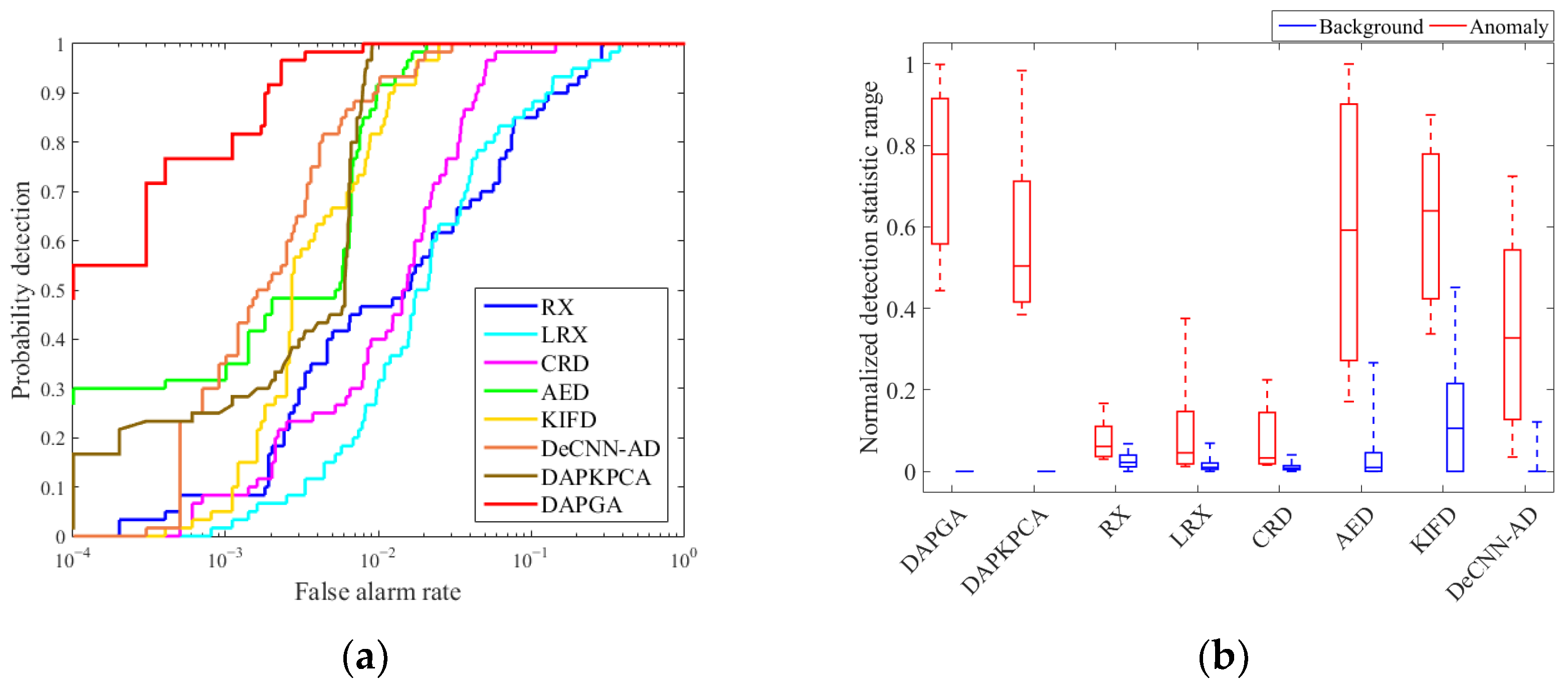
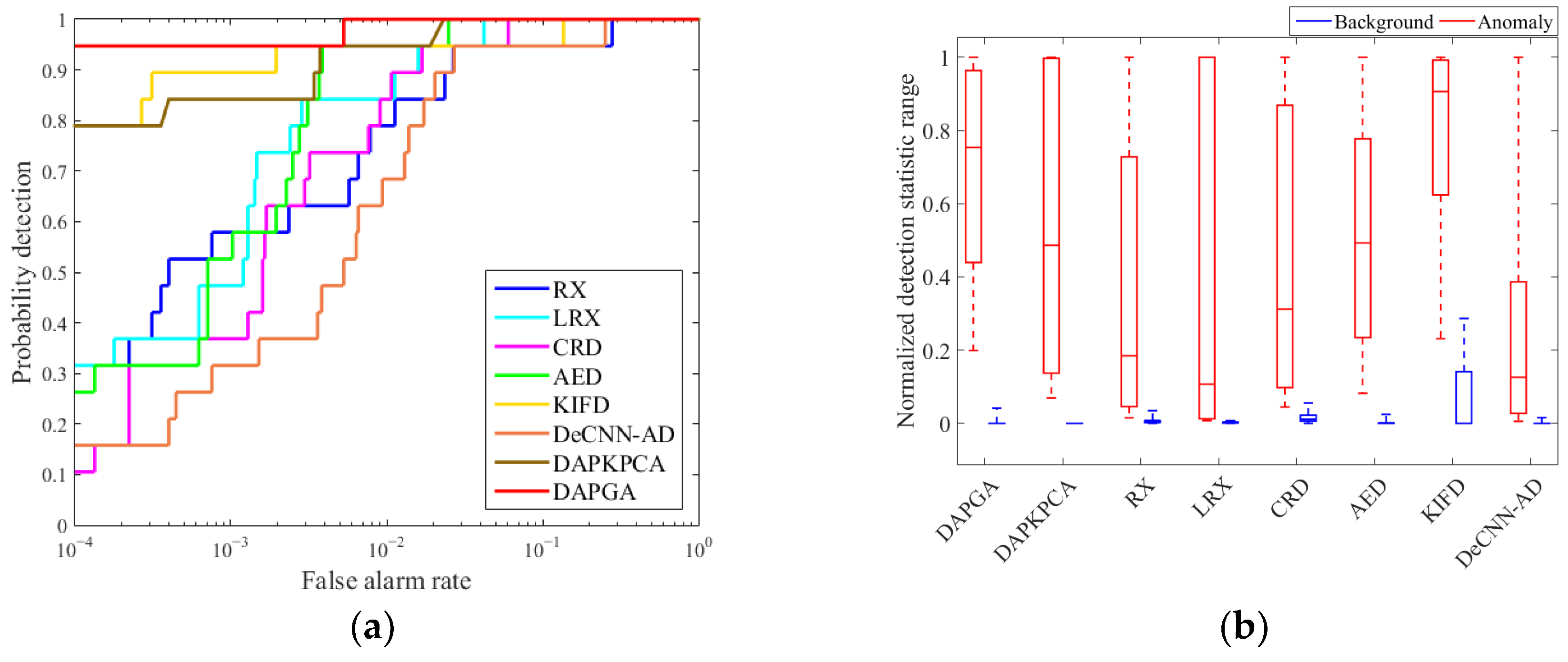
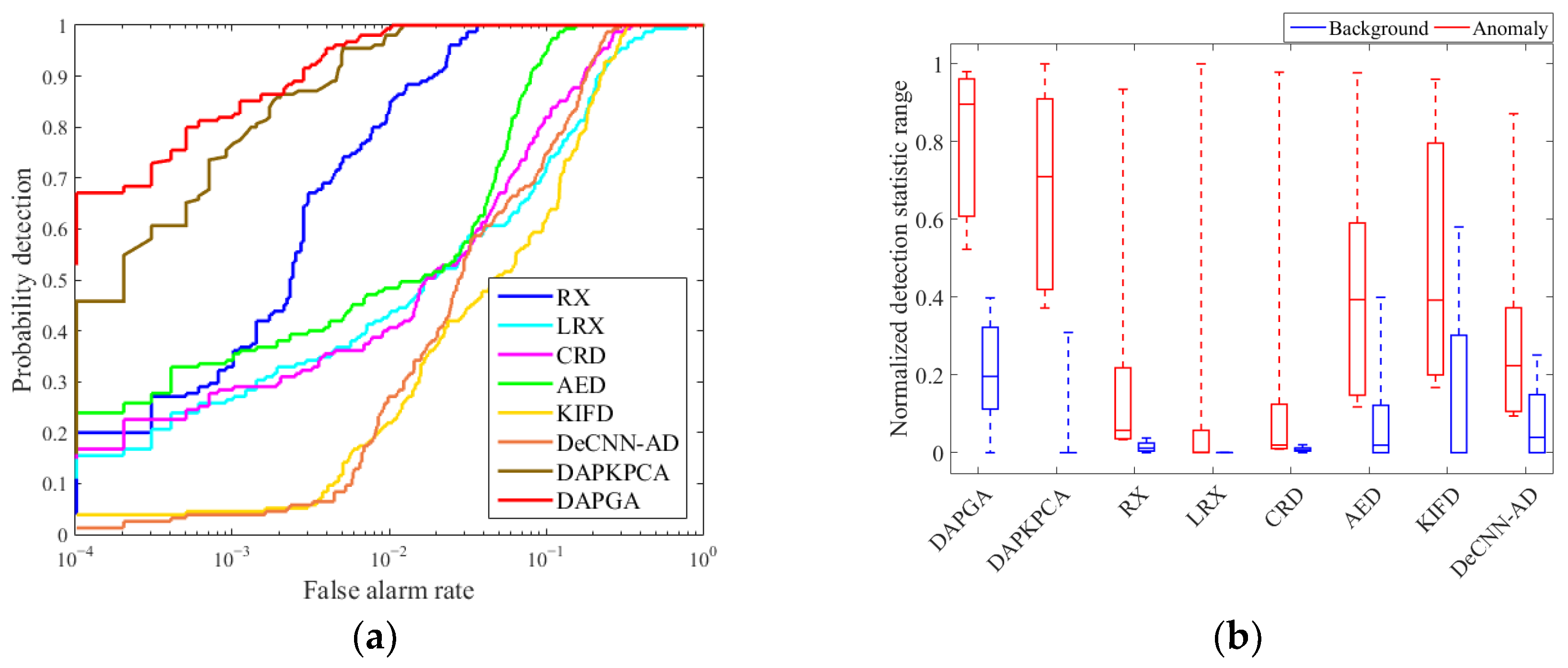
Four common metrics are employed to assess the detection capability qualitatively and quantitatively. The receiver operating characteristic (ROC) as the first metric reflects the corresponding relation between the probability of detection (PD) and the false alarm rate (FAR) at different thresholds on the basis of the ground truth. Typically, the superior detector is located closer to the upper left corner. The background–target separability maps are set as the second metric, which depicts the capacity to distinguish separating targets from the background and the background suppression effect. High separation and good background suppression between anomalies and background demonstrate the superb functionality of the detector. The third metric is the area under the curve (AUC), which refers to the total area under the ROC curve. Higher AUC values indicate better performance. Additionally, the running time is the fourth metric employed to evaluate the detection efficiency.

4.3. Experimental Settings

The LRX, CRD, AED, KIFD, DAPKPCA and DeCNN-AD methods require artificial adjustment of parameters to gain the greatest detection capability. Therefore, the optimal parameters are set relying on the AUC value in each dataset. The detection capabilities are sensitive to the window sizes (ωin and ωout) in the LRX and CRD methods, so the window sizes ωin ranging from 3 to 19 and ωout ranging from 5 to 23 are the main selection range. The regularization parameter λ is insensitive to the detection performance in CRD method, so this parameter is fixed as 10−6. Likewise, the parameters κ, δs and δr are sensitive in AED method. The area parameter κ is selected optimally, ranging from 5 to 300. The parameters δs and δr, which adjust the amount of smoothness in edge-preserving filtering, vary from 0.5 to 5. After performing principal component analysis, the reserved spectral number of the AED method is set to 3. In addition, the number range of principal components ζ is preset between 50 and 300 in the KIFD method. The Gaussian radial basis function (RBF) is used as the nonlinear kernel of KPCA in the DAPKPCA method, and the Gaussian parameter σ is from 5 to 100. The cluster number K of DeCNN-AD is selected between 2 and 12, and the parameters β and λ are chosen from among [0.00001, 0.0001, 0.001, 0.01, 0.1, 0.2, 0.3]. For the proposed DAPGA method, the number n of clustering centers representing the optimal differential attribute profiles is set from 10 to 55. The detailed optimal parameters of each method in every dataset are listed in Table 2. In this paper, the threshold number m in each attribute type for extracting the multi-scale spatial characteristics is given as five, and the typical band number b is four. The total number of differential attribute profiles is the product of typical band number b and attribute operator number, and these profiles are exploited as the individual in GAs for clustering. The number of attribute operators is set to twenty (four attribute types and five thresholds). Therefore, the total number of differential attribute profiles is eighty.

4.4. Detection Performance

The detection maps of each compared method are presented in Figure 4, Figure 5, Figure 6 and Figure 7. The RX detector is inclined to highlight the areas with a strong edge; thus, the shapes of some targets are lost, decreasing its detection accuracy. For the comparatively diverse and irregular anomalies, the LRX and CRD detectors are usually hard to identify all anomalous pixels. The AED detector can well detect the positions of anomalies, but the object edge is blurred, and it introduces some false pixels. For the KIFD detector, a portion of background is mistakenly classified as anomalous pixels as well as some detection maps contain serious noise. The DeCNN-AD method is good at suppressing uniform and pure backgrounds, and thus has fewer false alarms, but it lacks the capacity to highlight the anomaly targets. Owing to the advantage of multi-scale differential attribute profiles in detecting various scale objects, the proposed DAPGA and the DAPKPCA methods could completely and obviously distinguish the anomaly targets’ contours in different scenes. Furthermore, the DAPGA method makes anomalies more prominent and distinct than DAPKPCA. The Gulfport airport dataset is equipped with a comparatively complex background and multiple objects with different sizes and irregular shapes. The subtle difference in the digital number (DN) value between airport and airplanes increases the difficulty of detection. Nevertheless, the proposed DAPGA, DAPKPCA and AED methods outperform other methods in terms of detection performance. Due to equipping the character of smoothing and blurring the edge regions in the edge-preserving filtering step, the AED detector displays excellent detection capability in detecting complex and irregular shapes, but it also introduces more false alarm pixels. As exhibited in the Cat Island beach dataset, which contains one small target and a relatively simple background, the DAPGA method is superior to the compared methods, and it can effectively protrude the anomalies while penalizing the background. The Texas Coast urban dataset contains multiple homogeneous targets with different scales. The DAPGA method also can keep outstanding detection performance and higher robustness when HSIs contain serious noise, whereas the RX, KIFD and DeCNN-AD detectors are affected by the serious strip noise. Specifically, the targets in the Rochester park dataset are composed of different materials and colors, as well as only covering several pixels, while the DAPGA method still exhibits excellent detection capability. Moreover, the background suppression effect of DAPGA is superior to RX, AEDand KIFD. By comparing the detection results visually, the DAPGA method performs well in the field of noise suppression and highlights the anomalies with fewer false alarms.
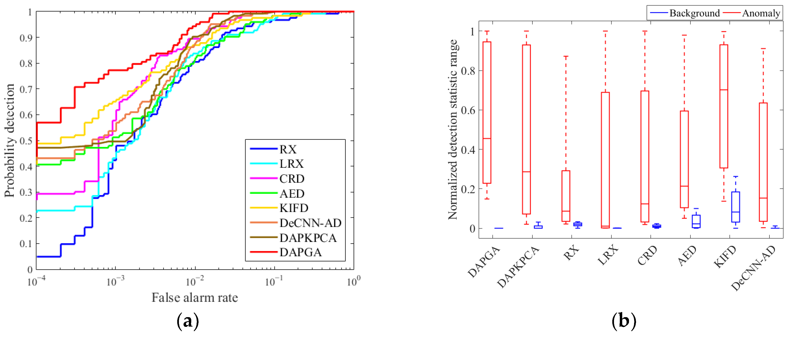
The ROC curves and background–target separability maps for the compared methods are displayed in Figure 8, Figure 9, Figure 10 and Figure 11, respectively. The Log10 coordinate is used for the ROC curves, and the curves of DAPGA method are higher than other compared methods in most cases when the false alarm rate is between 10−4 and 1. In contrast to other methods, the detection probability of DAPGA reaches roughly 0.82 and DAPKPCA is over 0.75 when the false alarm rate is fixed to a relatively low value (0.001) in Figure 10, while others are all less than 0.4. In addition, the detection rate of the DAPGA method is usually larger than 0.9 before the false alarm rate exceeds 0.01. As a consequence, the DAPGA method offers promising outcomes for a low false alarm rate.
The background–target separability maps are applied to examine the detection ability in the form of box plots. There are two boxes for each detector. The background and anomaly distribution are depicted by the blue and red boxes, respectively. The position of the boxes reflects the separability between the anomaly class and background class, and a larger separability distance denotes a better detection behavior. Additionally, background suppression is more effective when the background box is shorter. The DAPGA algorithm has a superior background suppression effect and better separability degree than others in various scenes containing targets of different sizes and materials, which means that the representation ability of the DAPDA algorithm is strong. In conclusion, the DAPDA algorithm can fully restrain the background, protrude anomalies, and distinguish the anomaly target from the background.
The corresponding AUC scores and the running time are listed in Table 3 and Table 4, where the optimum values are emphasized in bold. The AUC scores of DAPGA are 0.9986, 0.9996, 0.9993 and 0.9981, according to the sequence of datasets, and the average of all datasets reaches 0.9989, which is much higher than other compared approaches. Two AUCs are more elevated than 0.999 in the Beach and Urban datasets. The AUCs of DAPGA are much higher than the second-best approach, 0.9963 (DeCNN-AD), 0.9984 (DAPKPCA), 0.9988 (DAPKPCA) and 0.9958 (CRD). The minimum AUC scores of each detector are 0.9981 (DAPGA), 0.9957 (DAPKPCA), 0.9696 (AED), 0.9526 (RX), 0.9461 (CRD), 0.9366 (DeCNN-AD), 0.9231 (LRX) and 0.9121 (KIFD), which indicates that the DAPGA algorithm has the highest stability. Additionally, the DAPGA algorithm reaches a score that is about 3.4% higher than the LRX detector in the average of all datasets, which also confirms that the DAPGA algorithm exhibits excellent hyperspectral detection performances.
The efficiency of the aforementioned detectors are also contrasted on a computer with an Intel® Core (TM) i7-6500U CPU and 8GB memory. All experiments are performed in MATLAB software and the running time in seconds is exhibited in Table 4. The running time of the DAPGA method is much shorter than the DAPKPCA, LRX, CRD, KIFD and DeCNN-AD detectors and longer than the RX and AED detectors, whereas it has a superior detection performance. The differential operation of the attribute profile is employed in both the proposed DAPGA and AED methods to enlarge the details that are different from the background. Since edge-preserving filtering is introduced in the AED method, some distinct anomalous pixels are smoothed with their neighbors while refining target boundaries as illustrated in Figure 6, which is detrimental to the separation of the target and background as depicted in Figure 10. The DAPGA method fully uses the differential attribute profiles to extract the multi-type and multi-scale spectral–spatial features, which could describe anomalous targets more comprehensively than the AED method with only one scale area attribute filter. The DAPGA method also avoids manually adjusting and setting the “significant” filter parameters in the AED method, rather automatically selecting the representative and informative features by genetic algorithms. The fusion of these optimal features achieves detailed information complementary to enhance the detection capability further. Therefore, it outperforms other compared methods regarding the AUC scores and background–target separability degree. Additionally, the kernel matrix size of DAPKPCA is proportional to the dataset size M × N, so it is suitable for small size datasets. The time increases exponentially when the scale expands and the DAPKPCA occupies too many memory resources. For the DeCNN-AD method, it can be accelerated with GPU, and the efficiency will be improved by multiple fold.

4.5. Parameter Analysis

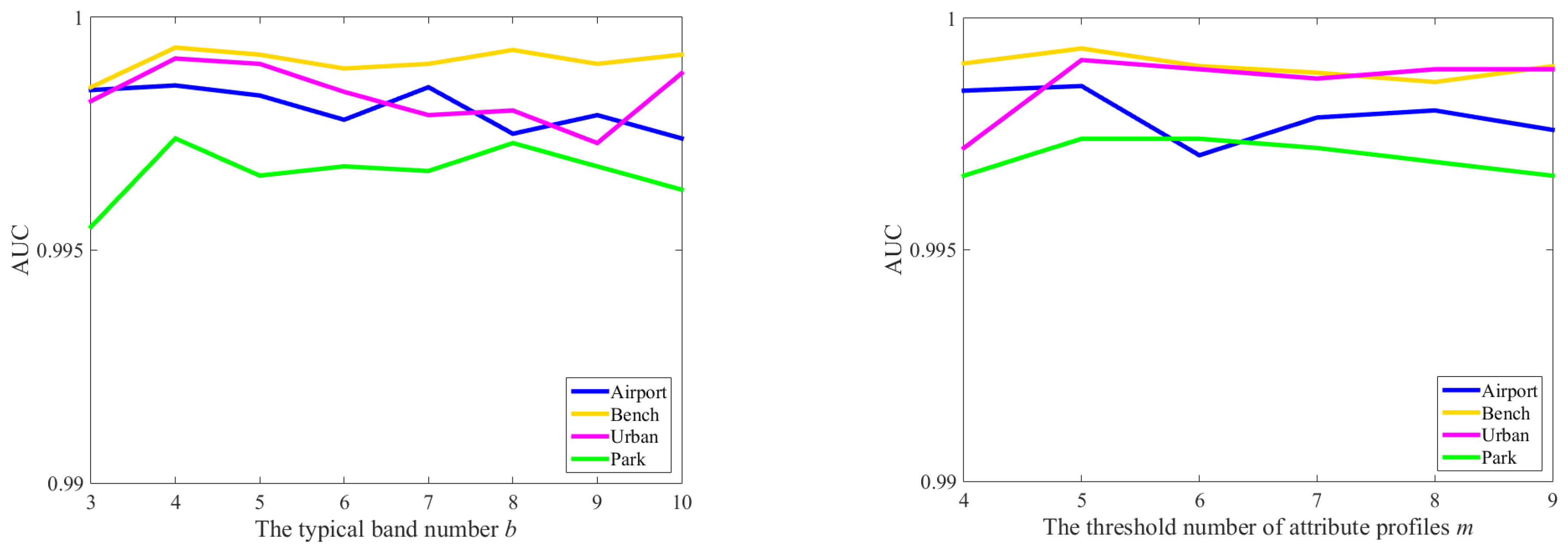
The influence of various parameters on the detection performance of the DAPGA method is analyzed in this section. The parameters contain the reserved typical band number b in band selection, the threshold number of attribute profiles m and the clustering center number n, representing the number of optimal DAPs. Figure 12 exhibits the effect of the parameters b, m and n over the AUC scores and running time of the DAPGA method on each dataset. When analyzing one of the parameters, the others will be set as default parameters b = 4, m = 5 and n = 40. As depicted in the top left of Figure 12, the AUC values tend to be stable in most situations when the band number b is larger than four. The top right of Figure 12 shows the influence of threshold number m in each attribute type over the detection performance. The AUC curve reaches a peak when m is equal to five and is generally smooth and stable. It means that the selection of a threshold number may have little impact on detection performance when the threshold number is greater than five. As shown in the bottom subfigures, the optimal number n of clustering centers for each dataset is quite different. In general, the DAPGA method demonstrates good detection performance when n is in the range of thirty-five to forty-five. Additionally, the computing time increases rapidly with the clustering center number n.

5. Discussion

This section mainly discusses the detection performance and application scope of the proposed DAPGA method based on the above results. In the aspect of selecting hyperspectral remote sensing dataset, the characteristics including the background complexity, target material, size and shape are mostly considered, thus four representative datasets in the different scenes are selected. The DAPGA method provides a high detection effect on targets with irregular shapes, as displayed in Figure 4 and Figure 5. The multi-scale and multi-type feature extraction structure makes the DAPGA method capable of detecting multiple targets with different scales simultaneously, and the detected targets have clear boundaries and do not stick together as indicated in Figure 6. The method still exhibits superior detection capability for different material targets located in the same scene in Figure 7. Additionally, we introduce four evaluation metrics for quantitative comparison. The ROC curves of DAPGA method are higher than other compared methods in most cases. In the box plots, the DAPGA method exhibits a larger separability distance between background and anomaly than other methods, which means a stronger capacity of restraining the background and protruding the anomalies. The average AUC of the DAPGA method (0.9989) is much higher than the second-best method (0.9972 for DAPKPCA), which also demonstrates that DAPs are good at multi-level feature extraction, and genetic algorithms are better than KPCA in selecting the optimal attribute profiles to achieve intelligent feature reduction. In conclusion, the proposed method can fully extract the spectral–spatial information of hyperspectral images and automatically select the optimal features, and most importantly it has brilliant detection results.
The genetic algorithms have some shortcomings in time complexity, because they require continuous iterative optimization, which has some impact on the running time of the proposed algorithm. The future direction of our research is optimizing the algorithm architecture to reduce its complexity. Furthermore, the strategies of attribute type selection and threshold range setting in the proposed method are mainly designed for anomaly targets, which are usually small in size and have a low proportion of pixels in the HSIs. However, for large-sized target detection or other applications, more selection strategies for general filtering parameters need to be explored and developed on a case-by-case basis.

6. Conclusions

A novel anomaly detection method with differential attribute profiles and genetic algorithms is proposed for hyperspectral images. The new DAPGA method could make the utmost of spectral and spatial information to distinguish anomaly targets. A main contribution of the differential attribute profiles is that they can extract multi-scale and multi-type spectral–spatial features and thus effectively highlight the anomaly objects, especially for different scales of objects. To alleviate the redundancy of feature information, the genetic algorithms are introduced to iteratively sort representative features from the constructed differential attribute profiles to weighted merge for generating the final detection map. The experiments on a variety of hyperspectral scenes confirm that the DAPGA method is quite competitive in terms of detection performance, algorithm stability and the background–target separability effect. An important aspect deserving of future research is the efficiency of the proposed architecture. In the future, refining the proposed method to shorten the running time while maintaining high performance will be the focus.

Author Contributions

Conceptualization, H.W. (Hanyu Wang), T.Z. and D.T.; methodology, H.W. (Hanyu Wang) and M.Y.; software, H.W. (Hanyu Wang); validation, H.W. (Hao Wang) and D.Y.; formal analysis, L.M.; investigation, T.Z. and H.S.; resources, H.W. (Hanyu Wang) and M.Y.; data curation, H.W. (Hanyu Wang) and T.Z.; writing—original draft preparation, H.W. (Hanyu Wang); writing—review and editing, M.Y., D.Y. and L.M.; supervision, D.T.; project administration, T.Z.; funding acquisition, H.S. All authors have read and agreed to the published version of the manuscript.

Funding

This research was funded by the Scientific research business fee fund of Heilongjiang provincial scientific research institutes, Research on Key Technologies of wide area forest and grass fire aerial monitoring and early warning (No. CZKYF2020B009) and the Key Technology R&D Program of JiLin Province (No. 20200403058SF).

Data Availability Statement

The hyperspectral datasets used in this study are available at http://xudongkang.weebly.com/; https://www.rit.edu/cos/share2012/downloads.php (accessed on 10 January 2022).

Acknowledgments

The authors would like to thank the Editor, Associate Editor, and Anonymous Reviewers for their helpful comments and suggestions to improve this paper, as well as the authors of the CRD, AED, KIFD and DeCNN-AD algorithms for sharing their codes. The authors would also like to give special thanks to X. Kang from Hunan University, for his assistance during the dataset collection.

Conflicts of Interest

The authors declare no conflict of interest.

References

  1. Mei, X.; Ma, Y.; Li, C.; Fan, F.; Huang, J.; Ma, J. Robust GBM hyperspectral image unmixing with superpixel segmentation based low rank and sparse representation. Neurocomputing 2018, 275, 2783–2797. [Google Scholar] [CrossRef]
  2. Kang, X.; Li, C.; Li, S.; Lin, H. Classification of hyperspectral images by Gabor filtering based deep network. IEEE J. Sel. Top. Appl. Earth Observ. Remote Sens. 2017, 11, 1166–1178. [Google Scholar] [CrossRef]
  3. Xie, W.; Lei, J.; Liu, B.; Li, Y.; Jia, X. Spectral constraint adversarial autoencoders approach to feature representation in hyperspectral anomaly detection. Neural Netw. 2019, 119, 222–234. [Google Scholar] [CrossRef]
  4. Ghamisi, P.; Yokoya, N.; Li, J. Advances in hyperspectral image and signal processing: A comprehensive overview of the state of the art. IEEE Geosci. Remote Sens. Mag. 2017, 5, 37–78. [Google Scholar] [CrossRef] [Green Version]
  5. Xie, W.; Liu, B.; Li, Y.; Lei, J.; Chang, C.-I.; He, G. Spectral adversarial feature learning for anomaly detection in hyperspectral imagery. IEEE Trans. Geosci. Remote Sens. 2020, 58, 2352–2365. [Google Scholar] [CrossRef]
  6. Reed, I.S.; Yu, X. Adaptive multiple-band CFAR detection of an optical pattern with unknown spectral distribution. IEEE Trans. Acoust. Speech Signal Process. 1990, 38, 1760–1770. [Google Scholar] [CrossRef]
  7. Matteoli, S.; Veracini, T.; Diani, M.; Corsini, G. A locally adaptive background density estimator: An evolution for RX-based anomaly detectors. IEEE Geosci. Remote Sens. Lett. 2014, 11, 323–327. [Google Scholar] [CrossRef]
  8. Chang, C.I.; Chiang, S.S. Anomaly detection and classification for hyperspectral imagery. IEEE Trans. Geosci. Remote Sens. 2002, 40, 1314–1325. [Google Scholar] [CrossRef] [Green Version]
  9. Kwon, H.; Nasrabadi, N.M. Kernel RX-algorithm: A nonlinear anomaly detector for hyperspectral imagery. IEEE Trans. Geosci. Remote Sens. 2005, 43, 388–397. [Google Scholar] [CrossRef]
  10. Gu, Y.; Liu, Y.; Zhang, Y. A Selective Kernel PCA Algorithm for Anomaly Detection in Hyperspectral Imagery. In Proceedings of the 2006 IEEE International Conference on Acoustics Speech and Signal Processing, Toulouse, France, 14–19 May 2006. [Google Scholar] [CrossRef]
  11. Guo, Q.; Zhang, B.; Ran, Q.; Gao, L.; Li, J.; Plaza, A. Weighted-RXD and linear filter-based RXD: Improving background statistics estimation for anomaly detection in hyperspectral imagery. IEEE J. Sel. Top. Appl. Earth Observ. Remote Sens. 2014, 7, 2351–2366. [Google Scholar] [CrossRef]
  12. Zhao, R.; Du, B.; Zhang, L. A robust nonlinear hyperspectral anomaly detection approach. IEEE J. Sel. Top. Appl. Earth Observ. Remote Sens. 2014, 7, 1227–1234. [Google Scholar] [CrossRef]
  13. Tao, R.; Zhao, X.; Li, W.; Li, H.; Du, Q. Hyperspectral anomaly detection by fractional Fourier entropy. IEEE J. Sel. Top. Appl. Earth Obs. Remote Sens. 2019, 12, 4920–4929. [Google Scholar] [CrossRef]
  14. Wei, L.; Qian, D. Collaborative representation for hyperspectral anomaly detection. IEEE Trans. Geosci. Remote Sens. 2015, 53, 1463–1474. [Google Scholar] [CrossRef]
  15. Ma, N.; Peng, Y.; Wang, S. A fast recursive collaboration representation anomaly detector for hyperspectral image. IEEE Geosci. Remote Sens. Lett. 2019, 16, 588–592. [Google Scholar] [CrossRef]
  16. Wu, Z. Hyperspectral anomaly detection with relaxed collaborative representation. IEEE Trans. Geosci. Remote Sens. 2022, 60, 1–17. [Google Scholar] [CrossRef]
  17. Chen, Y.; Nasrabadi, N.M.; Tran, T.D. Simultaneous joint sparsity model for target detection in hyperspectral imagery. IEEE Geosci. Remote Sens. Lett. 2011, 8, 676–680. [Google Scholar] [CrossRef]
  18. Zhao, X.; Li, W.; Zhang, M.; Tao, R.; Ma, P. Adaptive iterated shrinkage thresholding-based Lp-norm sparse representation for hyperspectral imagery target detection. Remote Sens. 2020, 12, 3991. [Google Scholar] [CrossRef]
  19. Huang, J.; Liu, K.; Li, X. Locality constrained low rank representation and automatic dictionary learning for hyperspectral anomaly detection. Remote Sens. 2022, 14, 1327. [Google Scholar] [CrossRef]
  20. Zhao, R.; Du, B.; Zhang, L. Hyperspectral anomaly detection via a sparsity score estimation framework. IEEE Trans. Geosci. Remote Sens. 2017, 55, 3208–3222. [Google Scholar] [CrossRef]
  21. Yao, W.; Li, L.; Ni, H.; Li, W.; Tao, R. Hyperspectral anomaly detection based on improved RPCA with non-convex regularization. Remote Sens. 2022, 14, 1343. [Google Scholar] [CrossRef]
  22. Zhao, C.; Wang, M.; Feng, S. Hyperspectral target detection method based on nonlocal self-similarity and rank-1 tensor. IEEE Trans. Geosci. Remote Sens. 2022, 60, 1–15. [Google Scholar] [CrossRef]
  23. Banerjee, A.; Burlina, P.; Diehl, C. A support vector method for anomaly detection in hyperspectral imagery. IEEE Trans. Geosci. Remote Sens. 2006, 44, 2282–2291. [Google Scholar] [CrossRef]
  24. Li, S.; Zhang, K.; Duan, P.; Kang, X. Hyperspectral anomaly detection with kernel isolation forest. IEEE Trans. Geosci. Remote Sens. 2020, 58, 319–329. [Google Scholar] [CrossRef]
  25. Song, X.; Aryal, S.; Ting, K.M.; Liu, Z.; He, B. Spectral-spatial anomaly detection of hyperspectral data based on improved isolation forest. IEEE Trans. Geosci. Remote Sens. 2022, 60, 1–16. [Google Scholar] [CrossRef]
  26. Xu, Y.; Zhang, L.; Du, B.; Zhang, L. Hyperspectral Anomaly Detection Based on Machine Learning: An Overview. IEEE J. Sel. Top. Appl. Earth Obs. Remote Sens. 2022, 15, 3351–3364. [Google Scholar] [CrossRef]
  27. Zhao, C.; Li, C.; Feng, S.; Li, W. Spectral-spatial anomaly detection via collaborative representation constraint stacked autoencoders for hyperspectral images. IEEE Geosci. Remote Sens. Lett. 2022, 19, 1–5. [Google Scholar] [CrossRef]
  28. Chen, Y.; Zhao, X.; Jia, X. Spectral-spatial classification of hyperspectral data based on deep belief network. IEEE J. Sel. Top. Appl. Earth Observ. Remote Sens. 2015, 8, 2381–2392. [Google Scholar] [CrossRef]
  29. Wu, K.; Zhu, L.; Shi, W.; Wang, W.; Wu, J. Self-attention memory-augmented wavelet-CNN for anomaly detection. IEEE Trans. Circuits Syst. Video Technol. 2022. early access. [Google Scholar] [CrossRef]
  30. Yousefan, M.; Najafabadi, H.E.; Amirkhani, H. Deep anomaly detection in hyperspectral images based on membership maps and object area filtering. Expert Syst. Appl. 2022, 191, 116200. [Google Scholar] [CrossRef]
  31. Arisoy, S.; Nasrabadi, N.M.; Kayabol, K. Unsupervised Pixel-Wise Hyperspectral Anomaly Detection via Autoencoding Adversarial Networks. IEEE Geosci. Remote Sens. Lett. 2022, 19, 5502905. [Google Scholar] [CrossRef]
  32. Xie, W. Unsupervised spectral mapping and feature selection for hyperspectral anomaly detection. Neural Netw. 2020, 132, 144–154. [Google Scholar] [CrossRef]
  33. Fu, X.; Jia, S.; Zhuang, L.; Xu, M.; Zhou, J.; Li, Q. Hyperspectral Anomaly Detection via Deep Plug-and-Play Denoising CNN Regularization. IEEE Trans. Geosci. Remote Sens. 2021, 59, 9553–9568. [Google Scholar] [CrossRef]
  34. Wang, S.; Wang, X.; Zhang, L.; Zhong, Y. Auto-AD: Autonomous hyperspectral anomaly detection network based on fully convolutional autoencoder. IEEE Trans. Geosci. Remote Sens. 2022, 60, 5503314. [Google Scholar] [CrossRef]
  35. Mura, M.D.; Benediktsson, J.A.; Waske, B.; Bruzzone, L. Morphological attribute profiles for the analysis of very high resolution images. IEEE Trans. Geosci. Remote Sens. 2010, 48, 3747–3762. [Google Scholar] [CrossRef]
  36. Huang, X.; Guan, X.; Benediktsson, J.A.; Zhang, L.; Li, J.; Plaza, A.; Mura, M.D. Multiple morphological profiles from multicomponent-base images for hyperspectral image classification. IEEE J. Sel. Topics Appl. Earth Observ. Remote Sens. 2014, 7, 4653–4669. [Google Scholar] [CrossRef]
  37. Pedergnana, M.; Marpu, P.R.; Mura, M.D.; Benediktsson, J.A.; Bruzzone, L. A novel technique for optimal feature selection in attribute profiles based on genetic algorithms. IEEE Trans. Geosci. Remote Sens. 2013, 51, 3514–3528. [Google Scholar] [CrossRef]
  38. Ghamisi, P.; Mura, M.D.; Benediktsson, J.A. A survey on spectral-spatial classification techniques based on attribute profiles. IEEE Trans.Geosci. Remote Sens. 2015, 53, 2335–2353. [Google Scholar] [CrossRef]
  39. Bhardwaj, K.; Patra, S. An unsupervised technique for optimal feature selection in attribute profiles for spectral-spatial classification of hyperspectral images. ISPRS J. Photogram. Remote Sens. 2018, 138, 139–150. [Google Scholar] [CrossRef]
  40. Fang, L.; He, N.; Li, S.; Ghamisi, P.; Benediktsson, J.A. Extinction profiles fusion for hyperspectral images classification. IEEE Trans. Geosci. Remote Sens. 2018, 56, 1803–1815. [Google Scholar] [CrossRef]
  41. Mura, M.D.; Benediktsson, J.A.; Waske, B.; Bruzzone, L. Extended profiles with morphological attribute filters for the analysis of hyperspectral data. Int. J. Rem. Sens. 2010, 31, 5975–5991. [Google Scholar] [CrossRef]
  42. Huang, J.; Liu, K.; Xu, M.; Perc, M.; Li, X. Background purification framework with extended morphological attribute profile for hyperspectral anomaly detection. IEEE J. Sel. Top. Appl. Earth Observ. Remote Sens. 2021, 14, 8113–8124. [Google Scholar] [CrossRef]
  43. Kang, X.; Zhang, X.; Li, S.; Li, K.; Li, J.; Benediktsson, J.A. Hyperspectral anomaly detection with attribute and edge-preserving filters. IEEE Trans. Geosci. Remote Sens. 2017, 55, 5600–5611. [Google Scholar] [CrossRef]
  44. Li, S.; Zhang, K.; Hao, Q.; Duan, P.; Kang, X. Hyperspectral anomaly detection with multiscale attribute and edge-preserving filters. IEEE Geosci. Remote Sens. Lett. 2018, 15, 1605–1609. [Google Scholar] [CrossRef]
  45. Pesaresi, M.; Benediktsson, J.A. A new approach for the morphological segmentation of high-resolution satellite imagery. IEEE Trans. Geosci. Remote Sens. 2001, 39, 309–320. [Google Scholar] [CrossRef] [Green Version]
  46. Breen, E.J.; Jones, R. Attribute openings, thinnings, and granulometries. Comp. Vis. Image Understand. 1996, 64, 377–389. [Google Scholar] [CrossRef]
  47. Jang, J.-S.R.; Sung, C.-T.; Mizutani, E. Neuro-Fuzzy and Soft Computing; Prentice-Hall: Hoboken, NJ, USA, 1997. [Google Scholar]
  48. MartÍnez-UsÓ, A.; Pla, F.; Sotoca, J.M.; GarcÍa-Sevilla, P. Clustering-based hyperspectral band selection using information measures. IEEE Trans. Geosci. Remote Sens. 2007, 45, 4158–4171. [Google Scholar] [CrossRef]
  49. Gu, Y.; Liu, Y.; Zhang, Y. A Selective KPCA Algorithm Based on High-Order Statistics for Anomaly Detection in Hyperspectral Imagery. IEEE Geosci. Remote Sens. Lett. 2008, 5, 43–47. [Google Scholar] [CrossRef]
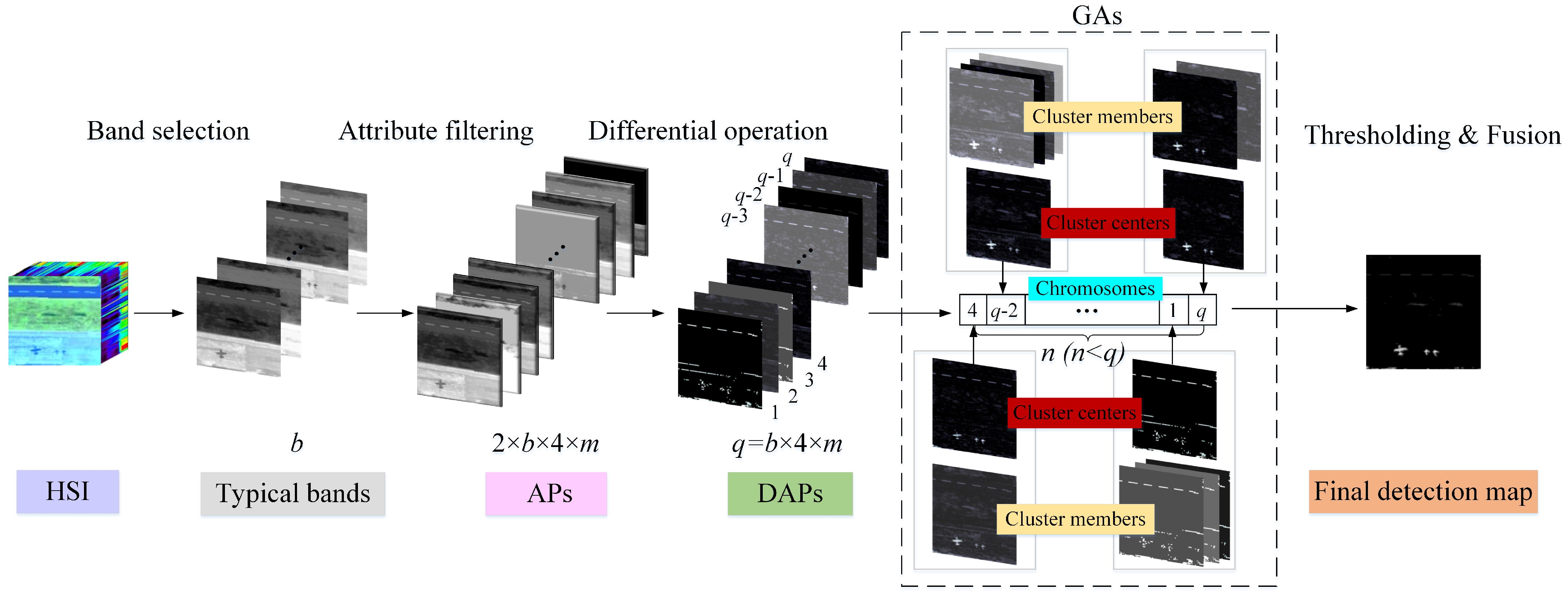
Figure 1. Schematic of the proposed method with differential attribute profiles and genetic algorithms.
Remotesensing 15 01050 g001
Figure 2. Graph of correlation coefficient matrix: (a) two-dimensional map; (b) three-dimensional map.
Remotesensing 15 01050 g002
Figure 3. Example of thickening, thinning and differential transformations with four attributes.
Remotesensing 15 01050 g003
Figure 4. The pseudocolor image, reference map and detection maps of the methods using the Gulfport airport dataset.
Remotesensing 15 01050 g004
Figure 5. The pseudocolor image, reference map and detection maps of the methods using the Cat Island beach dataset.
Remotesensing 15 01050 g005
Figure 6. The pseudocolor image, reference map and detection maps of the methods using the Texas Coast urban dataset.
Remotesensing 15 01050 g006
Figure 7. The pseudocolor image, reference map and detection maps of the methods using the Rochester park dataset.
Remotesensing 15 01050 g007
Figure 8. ROC curves and box plots of the methods using the Gulfport airport dataset: (a) receiver operating characteristic (ROC) curves; (b) background–target separability maps.
Remotesensing 15 01050 g008
Figure 9. ROC curves and box plots of the methods using the Cat Island beach dataset: (a) receiver operating characteristic (ROC) curves; (b) background–target separability maps.
Remotesensing 15 01050 g009
Figure 10. ROC curves and box plots of the methods using the Texas Coast urban dataset: (a) receiver operating characteristic (ROC) curves; (b) background–target separability maps.
Remotesensing 15 01050 g010
Figure 11. ROC curves and box plots of the methods using the Rochester park dataset: (a) receiver operating characteristic (ROC) curves; (b) background–target separability maps.
Remotesensing 15 01050 g011
Figure 12. Effects of the parameters b, m and n over the average AUCs and running time of the DAPGA method on each dataset.
Remotesensing 15 01050 g012aRemotesensing 15 01050 g012b
Table 1. Some features of four real hyperspectral datasets.
SceneCaptured PlaceSpatial ResolutionSizeSensor
AirportGulfport3.4 m/pixel100 × 100 × 191AVIRIS
BeachCat Island17.2 m/pixel150 × 150 × 188AVIRIS
UrbanTexas Coast17.2 m/pixel100 × 100 × 207AVIRIS
ParkRochester1 m/pixel100 × 100 × 360SpecTIR
Table 2. Optimal parameters of the DAPGA, DAPKPCA, LRX, CRD, AED, KIFD and DeCNN-AD methods over four datasets.
DatasetDAPGADAPKPCALRXCRDAEDKIFDDeCNN-AD
nσωinωoutωinωoutκδsδrζKβλ
Airport4010111313176450.520060.10.3
Beach401035352550.515060.010.1
Urban1520597916535040.20.1
Park501015171315165110040.010.2
Table 3. AUC scores of the methods over four datasets.
DatasetDAPGADAPKPCARXLRXCRDAEDKIFDDeCNN-AD
Airport0.99860.99570.95260.95380.98020.99530.99440.9963
Beach0.99960.99840.98070.99560.99370.99740.99280.9799
Urban0.99930.99880.99460.92310.94610.96960.91210.9366
Park0.99810.99570.98400.98710.99580.98990.99170.9794
Average0.99890.99720.97800.96490.97900.98810.97280.9730
Bold number are used to highlight which AUC score is the best among others in the row.
Table 4. Running time (seconds) of the methods over four datasets.
DatasetDAPGADAPKPCARXLRXCRDAEDKIFDDeCNN-AD
Airport22.7510.910.1449.1983.280.26127.90543.07
Beach24.51136.830.2586.9797.530.69113.22963.81
Urban21.3613.740.1559.3863.600.8985.15364.71
Park25.0414.590.27239.05257.210.2896.11274.96
Average23.4244.020.20108.65125.410.53105.60536.64
Bold number are used to highlight which running time is the best among others in the row.
Disclaimer/Publisher’s Note: The statements, opinions and data contained in all publications are solely those of the individual author(s) and contributor(s) and not of MDPI and/or the editor(s). MDPI and/or the editor(s) disclaim responsibility for any injury to people or property resulting from any ideas, methods, instructions or products referred to in the content.