Complex-Valued U-Net with Capsule Embedded for Semantic Segmentation of PolSAR Image

Abstract

In recent years, semantic segmentation with pixel-level classification has become one of the types of research focus in the field of polarimetric synthetic aperture radar (PolSAR) image interpretation. Fully convolutional network (FCN) can achieve end-to-end semantic segmentation, which provides a basic framework for subsequent improved networks. As a classic FCN-based network, U-Net has been applied to semantic segmentation of remote sensing images. Although good segmentation results have been obtained, scalar neurons have made it difficult for the network to obtain multiple properties of entities in the image. The vector neurons used in the capsule network can effectively solve this problem. In this paper, we propose a complex-valued (CV) U-Net with a CV capsule network embedded for semantic segmentation of a PolSAR image. The structure of CV U-Net is lightweight to match the small PolSAR data, and the embedded CV capsule network is designed to extract more abundant features of the PolSAR image than the CV U-Net. Furthermore, CV dynamic routing is proposed to realize the connection between capsules in two adjacent layers. Experiments on two airborne datasets and one Gaofen-3 dataset show that the proposed network is capable of distinguishing different types of land covers with a similar scattering mechanism and extracting complex boundaries between two adjacent land covers. The network achieves better segmentation performance than other state-of-art networks, especially when the training set size is small.

1. Introduction

Polarimetric synthetic aperture radar (PolSAR) can obtain rich information of the observed targets [1,2,3]. It has been widely used in agricultural monitoring, natural disaster assessment, biomass statistics, etc. The technologies of PolSAR image interpretation can help us understand and identify targets from an image; thus, it has always been a concern for researchers. However, since the formation mechanism of a PolSAR image is very complex, PolSAR image interpretation is still a challenging task. In recent years, driven by deep learning, two kinds of image interpretation technologies, namely image classification [4,5,6,7,8] and semantic segmentation [9,10,11], have made remarkable achievements.

PolSAR image classification based on deep learning has been deeply and extensively studied. According to the supervision mode, it mainly has three kinds of methods, namely, supervised, unsupervised, and semi-supervised [12]. For the supervised methods, convolutional neural networks (CNNs) [5,13] were the most widely used. Furthermore, a recursive neural network [14] was used. For the unsupervised methods, a deep belief network [15], an auto-encoder combined with Wishart distribution [16], and a task-oriented generative adversarial network [17] were studied. For the semi-supervised methods, a self-training model [18] and graph-based models [19,20] were proposed. In addition, some deep active learning and other new techniques were explored [21,22].

The research about CNN-based PolSAR image classification mainly focused on the real-valued (RV) structures and the inputs of networks at first. In terms of RV CNN structure, a four-layer CNN [23], a dual-branch deep CNN [24], a multi-channel fusion CNN [25], and a lightweight 3D CNN [26] were proposed. In terms of RV CNN inputs, some polarimetric features were selected to accelerate the convergence speed of CNN [13]. Then, complete features obtained by the polarimetric scattering coding were also used as the inputs [27]. Moreover, the amplitude and phase of the polarimetric coherence matrix were extracted as the inputs of a multi-task CNN [28]. Although both the methods of improving the network structure and extracting the complete input information effectively improved the classification performance, the problem of information loss caused by the RV structures and inputs still existed. Subsequently, some complex-valued (CV) CNNs were proposed to directly use the CV polarimetric coherent matrix as the input, aiming to avoid information loss. For example, a three-layer CV CNN [5], a CV 3D CNN [29], a CV 3D CNN combined with conditional random field [30], and a CV PolSAR-tailored differentiable architecture network [7] were widely studied. Furthermore, recurrent CV CNN combined with semi-supervised learning was also proposed for the classification with a small number of samples [31]. In the above classification processes, the training samples were obtained by using a sliding window, and each of them was an image patch with a small size. After the classification of each image patch, the obtained category was determined as the category of the center pixel in the patch. This pixel-by-pixel process had the problem of computational redundancy.

Semantic segmentation based on deep learning can achieve pixel-level classification in an end-to-end manner. Among various deep learning technologies, semantic segmentation networks based on s fully convolutional network (FCN) [32] have been rapidly developed. There are U-Net [33], SegNet [34], PSPNet [35], DeepLabv3+ [36], RefineNet [37], and so on. These networks have been used for semantic segmentation of optical [34,35,36,37], medical [33], and remote sensing images [38,39,40,41]. In the field of PolSAR image interpretation, semantic segmentation can effectively avoid the repeated computation when compared with image classification. Figure 1 shows the main differences between PolSAR image classification and semantic segmentation. For PolSAR image classification, the input is a small image patch that can be represented by a polarimetric coherent matrix, polarimetric decomposition results, and so on. The output is the category of the central pixel in the image patch. For semantic segmentation of a PolSAR image, the input is a large image block including multiple classes of targets, and its representation is the same as that of image classification. The output is the categories of all pixels in the image. Obviously, semantic segmentation can significantly reduce the computing time.

The research about semantic segmentation of PolSAR images started from FCN. Initially, FCN was only used to extract image features. Wang et al. used FCN to extract the spatial features and combined them with sparse and low-rank subspace features [42]. He et al. integrated FCN with a manifold graph embedding model to extract spatially polarized features [43]. After that, FCN, U-Net, SegNet, and DeepLabv3+ were applied in the semantic segmentation of PolSAR images in the real sense. Li et al. combined sliding window FCN with sparse coding to avoid the repeated calculations [44]. Mohammadimanesh et al. presented a new FCN with an encoder–decoder architecture for semantic segmentation of complex land cover ecosystems [45]. Pham et al. verified that SegNet could obtain promising segmentation results on very high-resolution PolSAR images [46]. Wu et al. used two structural modes (i.e., FCN and U-Net) and combined transfer learning strategies to perform semantic segmentation when the training set size was small [47]. Zhao et al. proposed a parallel dual-channel dilated FCN and used a semi-supervised fuzzy c-means clustering method to increase the number of the training samples [48]. Jing et al. proposed a polarimetric space reconstruction network, which included a scattering and polarimetric coherency coding module, a statistics enhancement module, and a dual self-attention convolutional network [49]. In order to fully utilize both amplitude and phase information of PolSAR data, Cao et al. presented a novel CV FCN [50], and Yu et al. proposed a lightweight CV Deeplabv3+ (L-CV-Deeplabv3+) [51].

The above CNN-based PolSAR image classification and FCN-based semantic segmentation greatly promoted the development of PolSAR image interpretation. However, there is still room for improvement due to the inherent defects of CNN. Taking face recognition as an example, even if the relative position of human eyes and mouth in an image is incorrect, CNN still recognizes it as a face because it is difficult for CNN to learn the relative positions between different entities in an image. A capsule network, which uses a vector neuron as the basic unit, can learn more information than CNN [52]. The amplitude of one activity vector neuron represents the probability of the existence of entities, and the orientation expresses instantiation parameters. Regarding the face recognition example, the capsule network can obtain the relative position between human eyes and the mouth, thus correctly recognizing the face. Furthermore, since vector neurons contain multiple properties of entities in the image, the capsule network requires fewer training samples than CNN during the training process. Up to now, the capsule network has also been widely used in optical [53,54], medical [55,56], remote sensing [57], and other image interpretation fields [58]. In the field of PolSAR image classification, Cheng et al. proposed a hierarchical capsule network to extract deep and shallow features. Experimental results on datasets from different platforms showed that the network had good generalization performance [59]. In the field of medical image semantic segmentation, Lalonde et al. proposed a segmented capsule network with U-shaped structure. Experimental results on pathological lungs showed that this network not only had better segmentation performance but also involved fewer parameters than U-Net [60].

In this paper, based on our previous work [61], we propose a CV U-Net with a capsule network embedded for semantic segmentation of PolSAR images. The reason for using U-Net as the backbone network is that its simple structure has good performance on small datasets when compared with other FCN-based segmentation networks. Considering that the PolSAR datasets used in this paper are small, the structure of U-Net is further lightweight to match these datasets. Moreover, U-Net is extended to the CV domain to directly use CV PolSAR data as the input. This CV network can mine the characteristics of the target from CV data, avoiding loss of information. In order to improve the feature extraction ability of the network, a CV capsule network is added behind the encoder of the CV U-Net. The CV capsule network mainly includes the CV primary capsules and the segmented capsules, which are different from those given in [52]. Inspired by [60], we also propose a locally constrained CV dynamic routing mechanism to realize the connection between capsules in two adjacent layers. The main contributions of this paper can be concluded as follows.

• A lightweight CV U-Net is designed for semantic segmentation of PolSAR image. It uses a polarimetric coherence matrix as the input of the network, aiming to utilize both the amplitude and phase information of PolSAR data. The lightweight structure of the network can match the PolSAR datasets with a small number of training samples.
• A CV capsule network is embedded between the encoder and decoder of CV U-Net to extract abundant features of PolSAR image. To make the CV capsule network suitable for semantic segmentation, the segmented capsule is adopted to replace the digital capsule used in the image classification.
• The locally constrained CV dynamic routing is proposed for the connection between capsules in two adjacent layers. The locally constrained characteristic helps to extend the dynamic routing to the connection of capsules with large sizes, and the routing consistency of the real part and imaginary part of the CV capsules improves the correctness of the extracted entity properties.
• Experiments on two airborne datasets and one Gaofen-3 PolSAR dataset verify that the proposed network can achieve better segmentation performance than other RV and CV networks, especially when the training set size is small.

The rest of this paper is organized as follows. The theoretical background about PolSAR data, U-Net and the capsule network are introduced in Section 2. Section 3 proposes a CV U-Net with capsule embedded and illustrates the principle of locally constrained CV dynamic routing. Experimental results and analysis are shown in Section 4. Section 5 discusses the improvement of segmentation performance brought by the CV capsule network. Finally, the conclusion is given in Section 6.

2. Related Work

2.1. PolSAR Data

Because PolSAR systems can transmit and receive different polarimetric electromagnetic waves, they can obtain rich scattering information about the observed targets. H and V are denoted as the horizontal and vertical polarization modes, respectively. Then, a 2 × 2 complex polarimetric scattering matrix can be written by,

$$[S]=\left[\begin{array}{cc}{S}_{HH}& S_{HV}\\ S_{VH}& S_{VV}\end{array}\right]$$

(1)

where the subscripts x and y of $S_{xy}$ (x = H, V; y = H, V) represent the polarization modes of the received and transmitted electromagnetic wave, respectively.

From the reciprocity theorem, $S_{HV}$ is approximately equal to $S_{VH}$ for monostatic SAR. Then, the scattering vector under Pauli basis can be expressed by,

$$k=\frac{1}{\sqrt{2}}{\left[S_{HH}+S_{VV},S_{HH}-S_{VV},2S_{HV}\right]}^T$$

(2)

Furthermore, the polarimetric coherence matrix $T$ is calculated by,

$$T=〈k\cdot k^H〉=\left[\begin{array}{ccc}{T}_{11}& T_{12}& T_{13}\\ T_{21}& T_{22}& T_{23}\\ T_{31}& T_{32}& T_{33}\end{array}\right]$$

(3)

2.2. U-Net

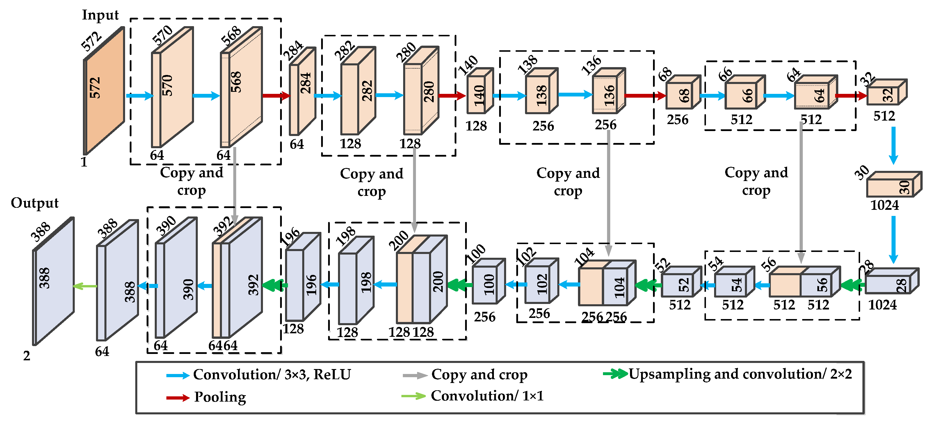
U-Net was first applied to semantic segmentation of medical images. The structure of U-Net proposed in [33] is shown in Figure 2. The upper part of the figure is the encoder, while the lower part is the decoder. They are almost symmetrical. The purpose of the encoder is to extract deep features, while the purpose of the decoder is to obtain target areas in the image and then determine their categories.

The encoder is also named the contracting path, because its feature sizes are gradually decreasing. It mainly includes four blocks, and each block contains two convolutional layers and one max pooling layer. From the second block, the first convolutional layer doubles the feature channels, and the maximum pooling layer halves the feature size. The decoder is also named the expanding path, because its feature sizes are gradually increasing. Corresponding to the encoder, it also includes four blocks. Each block contains one upsampling and convolutional layer and two convolutional layers. The upsampling and convolutional layer doubles the feature sizes and halves the feature channels. After the upsampling and convolution operation, the feature maps are concatenated with those copied and clipped from the corresponding encoder layer, aiming to restore good details of targets in the image. Then, the following convolutional layer halves the feature channels.

For all the convolutional operations in the network, the sizes of convolutional kernels are 3 × 3, and the convolutional stride is 1. After each convolutional operation, the ReLU activation function is used. The size of the pooling operation is 2 × 2, and the pooling stride is 2. For all the upsampling and convolution operations, the upsampling ratio is 2 × 2, and the size of the convolutional kernels is 2 × 2. After the last convolutional layer in the expansion path, there is one 1 × 1 convolution to obtain the categories of all targets in the image.

2.3. Capsule Network

A capsule network can overcome the shortcomings of CNN and obtain multiple properties of entities in the image. The architecture of the capsule network proposed in [52] is shown in Figure 3. It mainly includes two convolutional layers and one fully connected layer. The first convolutional layer is used in extracting features. The convolutional kernel has a size of 9 × 9, and the convolutional stride is 1. After the convolution operation, a ReLU activation function is used. The second convolutional layer is used in obtaining the primary capsules. The convolutional kernel also has a size of 9 × 9, and the convolutional stride is 2. The output of this layer is 32 × 6 × 6 primary capsules, and each primary capsule is a vector with size of 1 × 8. The final layer is used in obtaining the digital capsules, which connects the primary capsules through dynamic routing. The total number of digital capsules is 10, and each digital capsule is a vector with a size of 1 × 16. Finally, the category of sample is the number of the digital capsule whose value has the maximum under L2-norm.

3. Methodology

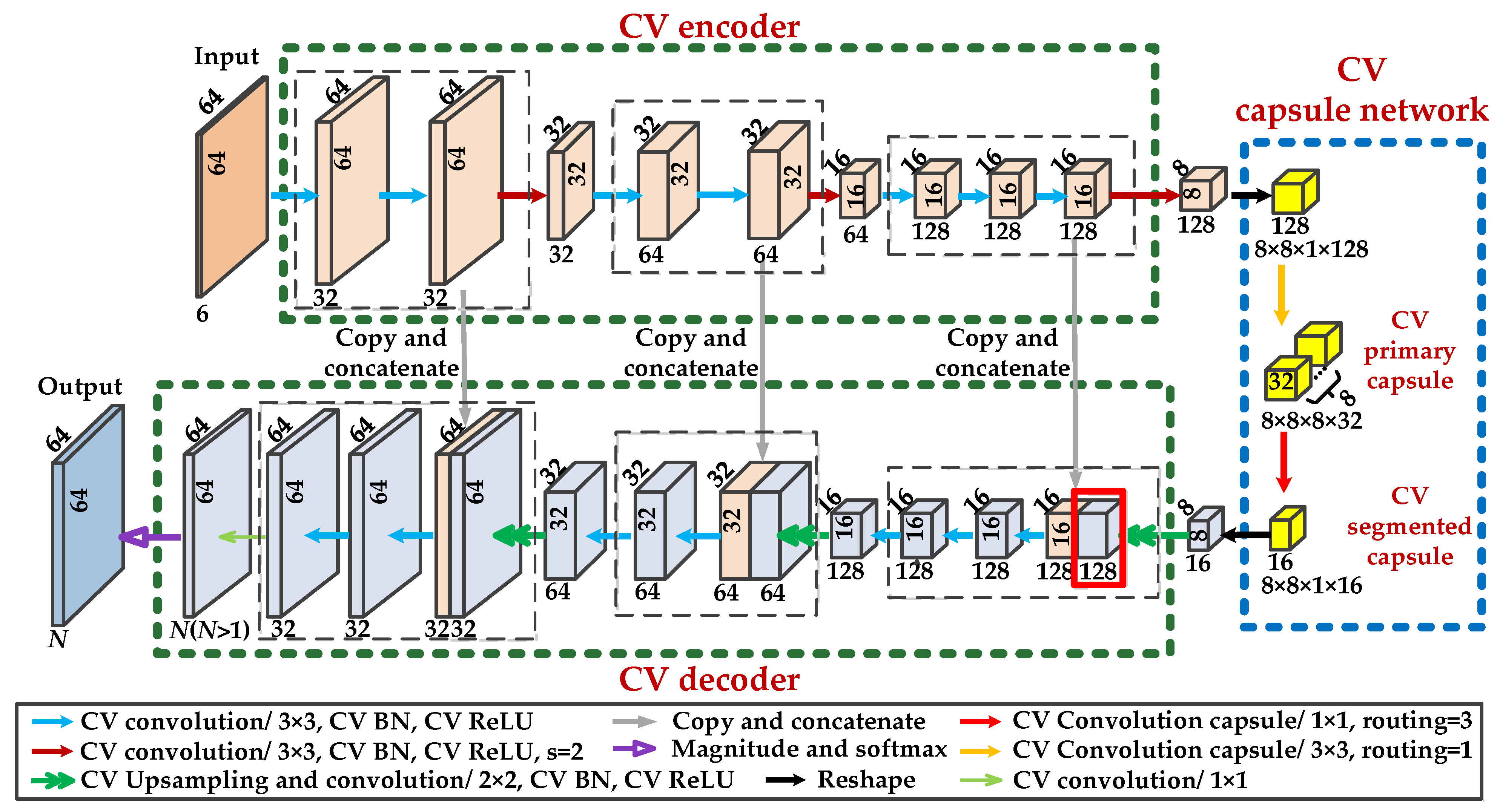
A CV U-Net with a capsule embedded is proposed for semantic segmentation of the PolSAR image in this section. The architecture of this network is shown in Figure 4. It mainly includes the CV encoder, CV decoder and CV capsule network, where the CV capsule network is embedded between the encoder and the decoder. Furthermore, the locally constrained CV dynamic routing is proposed for the connection between capsules in two adjacent layers of the CV capsule network. The detailed structure of the three parts and the principle of the locally constrained CV dynamic routing are introduced as follows.

3.1. CV Encoder

The CV encoder shown in Figure 4 (the green dashed box at the top) includes three CV convolutional blocks. For the first block, there are three CV convolutional layers in total. Each of the first two CV convolutional layers has 32, 3 × 3 convolution kernels, and the convolutional stride is 1. The output sizes of these two convolutional layers are the same as the input. The third CV convolutional layer has 32, 3 × 3 convolution kernels, and the convolutional stride is 2. The output size of this layer is half of the input. For the second block, the structure and convolution parameters are the same as those of the first block except that the number of convolution channels of each layer is twice that of the corresponding layer in the first block. For the third block, there are a total of four CV convolutional layers. Compared with the second block, it adds a convolution layer and doubles the convolution channels for each corresponding layer. Both a CV ReLU activation function and a CV batch normalization operation are located after each convolution operation. Formulas about the CV convolution operation and the CV ReLU activation function as well as the CV batch normalization method are provided in [62].

Regarding the structure of the CV encoder, it was designed based on the RV encoder shown in Figure 2. However, there are several differences between the CV and RV encoders. First, the number of convolutional blocks and convolution channels of the CV encoder are less than those of the RV encoder, so as to make the network fit for the small PolSAR datasets. Second, all the network parameters and convolution operations involved in the CV encoder are extended to the CV domain, which aims to extract more abundant information from the CV input. Third, the CV convolution with a stride of 2 in the CV encoder replaces the pooling operation in the RV encoder, which can reduce the loss of information. Finally, the mode of convolution with a stride of 1 in the CV encoder is different from that in the RV encoder. The output size obtained in the CV encoder is consistent with the input.

3.2. CV Decoder

The CV decoder shown in Figure 4 (the green dashed box at the bottom) includes three CV deconvolutional blocks, which are symmetrical to the CV encoder. For the first deconvolutional block, there are one CV upsampling and convolutional layer and three CV convolutional layers. The CV upsampling and convolutional layer has an upsampling ratio of 2 × 2, and the output size is twice the input. Then, a copy and concatenation operation is performed to combine low-level feature maps from the encoder with deep-level feature maps from the decoder. Next, three convolutional layers all have 128, 3 × 3 convolution kernels with a stride of 1. The output sizes of these convolutional layers are the same as the input. For the second deconvolutional block, it reduces one CV convolutional layer and halves the convolution channels of each layer when compared with the previous block. For the third CV deconvolutional block, the structure and convolution parameters are the same as those of the second block except for the convolution channels. There are also a CV ReLU activation and a CV batch normalization operation after each of the aforementioned convolution operation. After these three deconvolutional blocks, there is one CV convolution operation with a size of 1 × 1, which aims to make the convolution channels consistent with the total number of categories in the image. Subsequently, magnitude operation is implemented to covert CV features into RV. Finally, the softmax operation is used to complete the classification. Formulas about the upsampling operation, the concatenation, and the magnitude operation are provided in [51].

Comparing the above CV decoder with the RV decoder shown in Figure 2, there are also four differences. The first two differences are the same as those analyzed in the CV encoder. The third difference is that the magnitude operation is added in the CV decoder to directly use the RV softmax function for the classification. The last one is that the segmentation task of two categories in the RV decoder is extended to N (N > 1) categories in the CV decoder.

3.3. CV Capsule Network

The CV capsule network shown in Figure 4 (the blue dashed box) is embedded between the encoder and the decoder. The design of this structure is inspired by [60]. It mainly includes two CV convolution capsule layers and two reshape operations. At first, 128 feature maps with size of 8 × 8 are reshaped into 8 × 8 × 1, which can also be seen as 128 × 8 capsules with size of 1 × 8. Then, the CV primary capsules are obtained by the first convolution capsule layer. There are 32 × 8 × 8 primary capsules, and each primary capsule is a vector with size of 1 × 8. The connection between the previous feature maps in a vector form and the CV primary capsules adopts the locally constrained CV dynamic routing way introduced in Section 3.4. Next, the CV segmented capsules are obtained by the second convolution capsule layer. There are 16 × 8 segmented capsules with size of 1 × 8. The locally constrained CV dynamic routing is also used to connect the CV primary capsules and the segmented capsules. Finally, the segmented capsule is reshaped into 16 feature maps with size of 8 × 8, and it is used as the input of the CV decoder.

From the above structure and operations of the CV capsule network, it is obviously different from the original capsule network shown in Figure 3. In order to make the CV capsule network suitable for the semantic segmentation, the segmented capsule replaces the digital capsule used in the image classification. Furthermore, the convolution capsule operation instead of the fully connected operation is used in obtaining the segmented capsule. Because the convolution operation can share weight parameters, it is beneficial to reduce the amount of calculation. Furthermore, the locally constrained CV dynamic routing is used for the connection between capsules in two adjacent layers. It is helpful to extend the dynamic routing to capsules with large sizes. More importantly, the routing consistency of the real part and imaginary part of the CV capsules can improve the correctness of the extracted entity properties from the PolSAR image.

3.4. Locally Constrained CV Dynamic Routing

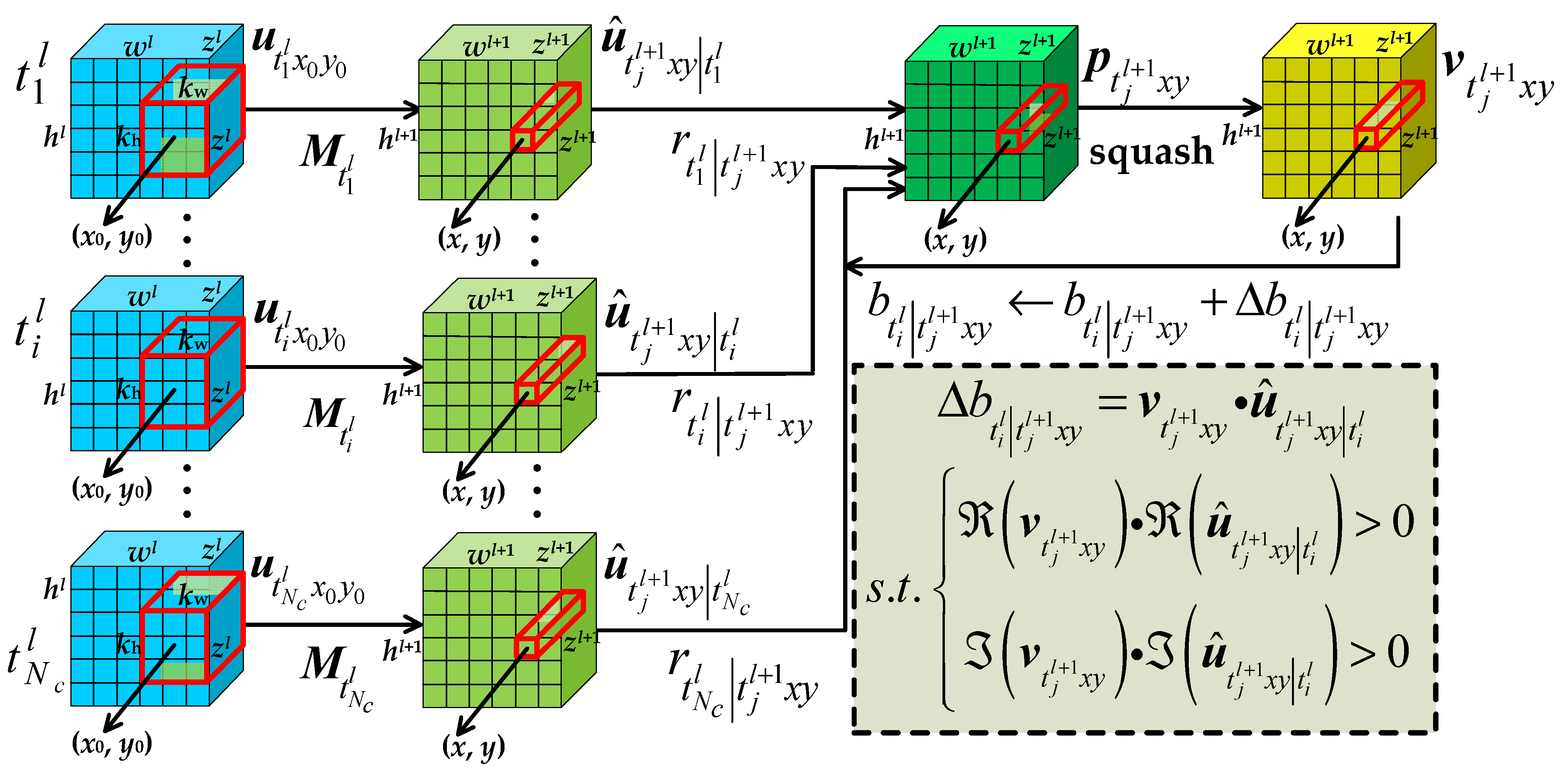
For any layer l ($l\ge 1$) and its adjacent layer l + 1 in the CV capsule network, suppose there are N_c types of CV child capsules at layer l and N_p types of CV parent capsules at layer l + 1. Denote the CV child capsule types as $T^l=\left\{t_1^l,t_2^l,\dots ,t_i^l\dots ,t_{N_c}^l\right\}$ and the CV parent capsule types as $T^{l+1}=\left\{t_1^{l+1},t_2^{l+1},\dots ,t_j^{l+1}\dots ,t_{N_{\mathit{p}}}^{l+1}\right\}$. For each $t_i^l\in T^l$, there are $h^l\times w^l$ child capsules with dimension of $z^l$. For each $t_j^{l+1}\in T^{l+1}$, there are $h^{l+1}\times w^{l+1}$ parent capsules with dimension of $z^{l+1}$. All the parent capsules can also be expressed by $P=\left\{{\mathit{p}}_{t_j^{l+1}11},\dots ,{\mathit{p}}_{t_j^{l+1}1w^{l+1}},\dots ,{\mathit{p}}_{t_j^{l+1}{h}^{l+1}1},\dots ,{\mathit{p}}_{t_j^{l+1}{h}^{l+1}{w}^{l+1}}\right\}$. Take a CV parent capsule ${\mathit{p}}_{t_j^{l+1}xy}\in P$ ($1\le x\le h^{l+1};1\le y\le w^{l+1}$), for example, the principle of locally constrained CV dynamic routing is shown in Figure 5, and the detailed process of child capsules routing to parent capsules is analyzed as follows.

At first, in a user-defined kernel (the red solid box), the CV convolution operation implemented by matrix multiplication is used in obtaining the prediction vectors. For a type of $t_i^l$ child capsules, a CV kernel with size of $k_h\times k_w\times z^l$ is defined as ${\mathit{u}}_{t_i^l{x}_0{y}_0}$, where $\left(x_0,y_0\right)$ is the center of the kernel. The CV matrix with size of $k_h\times k_w\times z^l\times N_p\times z^{l+1}$ is denoted as ${\mathit{M}}_{t_i^l}$, which is shared over all the kernels in the same type of CV child capsules. Therefore, the predicted CV vector ${\widehat{\mathit{u}}}_{t_j^{l+1}xy\left|t_i^l\right.}$ can be calculated by,

$${\widehat{\mathit{u}}}_{t_j^{l+1}xy\left|t_i^l\right.}={\mathit{M}}_{t_i^l}{\mathit{u}}_{t_i^l{x}_0{y}_0}$$

(4)

Then, the weighted sum over the predicted vectors from all the types of CV child capsules is implemented to obtain the CV parent capsule ${\mathit{p}}_{t_j^{l+1}xy}$, which can be expressed by,

$${\mathit{p}}_{t_j^{l+1}xy}={\displaystyle \sum _i{r}_{t_i^l\left|t_j^{l+1}xy\right.}{\widehat{\mathit{u}}}_{t_j^{l+1}xy\left|t_i^l\right.}}$$

(5)

where $r_{t_i^l\left|t_j^{l+1}xy\right.}$ is the routing coefficient. It can be calculated by,

$$r_{t_i^l\left|t_j^{l+1}xy\right.}=\frac{\exp \left(b_{t_i^l\left|t_j^{l+1}xy\right.}\right)}{{\displaystyle \sum _k\exp \left(b_{t_i^l\left|t_j^{l+1}k\right.}\right)}}$$

(6)

where $b_{t_i^l\left|t_j^{l+1}xy\right.}$ is the log prior probability.

Next, the squashed CV parent capsule ${\mathit{v}}_{t_j^{l+1}xy}$ is obtained by,

$${\mathit{v}}_{t_j^{l+1}xy}=\frac{{‖{\mathit{p}}_{t_j^{l+1}xy}‖}^2}{1+{‖{\mathit{p}}_{t_j^{l+1}xy}‖}^2}\frac{{\mathit{p}}_{t_j^{l+1}xy}}{‖{\mathit{p}}_{t_j^{l+1}xy}‖}$$

(7)

where

$$‖{\mathit{p}}_{t_j^{l+1}xy}‖=\sqrt{{‖\Re \left({\mathit{p}}_{t_j^{l+1}xy}\right)‖}^2+{‖\Im \left({\mathit{p}}_{t_j^{l+1}xy}\right)‖}^2}.$$

(8)

Finally, the coefficient $b_{t_i^l\left|t_j^{l+1}xy\right.}$ is updated by,

$$b_{t_i^l\left|t_j^{l+1}xy\right.}\leftarrow b_{t_i^l\left|t_j^{l+1}xy\right.}+\Delta b_{t_i^l\left|t_j^{l+1}xy\right.}.$$

(9)

where $\Delta b_{t_i^l\left|t_j^{l+1}xy\right.}$ is obtained by,

$$\Delta b_{t_i^l\left|t_j^{l+1}xy\right.}=\left\{\begin{array}{cc}{\mathit{v}}_{t_j^{l+1}xy}·{\widehat{\mathit{u}}}_{t_j^{l+1}xy\left|t_i^l\right.}& \begin{array}{l}\Re \left({\mathit{v}}_{t_j^{l+1}xy}\right)·\Re \left({\widehat{\mathit{u}}}_{t_j^{l+1}xy\left|t_i^l\right.}\right)>0\\ and \Im \left({\mathit{v}}_{t_j^{l+1}xy}\right)·\Im \left({\widehat{\mathit{u}}}_{t_j^{l+1}xy\left|t_i^l\right.}\right)>0\end{array}\\ 0& otherwise\end{array}\right.$$

(10)

Equation (10) means that only when the product of the real parts of ${\mathit{v}}_{t_j^{l+1}xy}$ and ${\widehat{\mathit{u}}}_{t_j^{l+1}xy\left|t_i^l\right.}$ is greater than 0 and the product of the imaginary parts of these two CV vectors is also greater than 0, $\Delta b_{t_i^l\left|t_j^{l+1}xy\right.}$ is equal to the dot product of ${\mathit{v}}_{t_j^{l+1}xy}$ and ${\widehat{\mathit{u}}}_{t_j^{l+1}xy\left|t_i^l\right.}$. Otherwise, $\Delta b_{t_i^l\left|t_j^{l+1}xy\right.}$ is equal to 0. This update condition is stricter than that of RV dynamic routing, because the coefficient is updated only when the dynamic routing of the real part is consistent with that of the imaginary part.

The above process of locally constrained CV dynamic routing can also be summarized in Algorithm 1.

Algorithm 1 Locally Constrained CV Dynamic Routing

1: Procedure Routing (${\widehat{\mathit{u}}}_{t_j^{l+1}xy\left|t_i^l\right.}$, d, l, $k_h$, $k_w$)

2:    for all CV child capsule types $t_i^l$ within a $k_h\times k_w$ kernel in layer l and a CV parent capsule $t_j^{l+1}xy$ in layer l + 1: $b_{t_i^l\left|t_j^{l+1}xy\right.}\leftarrow 0$.

3:    while iteration < d do

4:      for all CV child capsule types $t_i^l$ in layer l:

5:        $r_{t_i^l\left|t_j^{l+1}xy\right.}\leftarrow soft\max \left(b_{t_i^l\left|t_j^{l+1}xy\right.}\right)$ $\hspace{1em} \hspace{1em}⊳$ softmax computes Equation (6)

6:      for the CV capsule $t_j^{l+1}xy$ in layer l + 1:

7:        ${\mathit{p}}_{t_j^{l+1}xy}\leftarrow {\displaystyle \sum _j{r}_{t_i^l\left|t_j^{l+1}xy\right.}{\widehat{\mathit{u}}}_{t_j^{l+1}xy\left|t_i^l\right.}}$

8:      for the CV capsule $t_j^{l+1}xy$ in layer l + 1:

9:        ${\mathit{v}}_{t_j^{l+1}xy}\leftarrow squash\left({\mathit{p}}_{t_j^{l+1}xy}\right)$ $\hspace{1em}\hspace{1em}\hspace{1em}\hspace{1em}⊳$ squash computes Equation (7)

10:       for all CV capsule types $t_i^l$ and the CV capsule $t_j^{l+1}xy$:

11:        $b_{t_i^l\left|t_j^{l+1}xy\right.}\leftarrow b_{t_i^l\left|t_j^{l+1}xy\right.}+\Delta b_{t_i^l\left|t_j^{l+1}xy\right.}$ $\hspace{1em} \hspace{1em}⊳$$\Delta b_{t_i^l\left|t_j^{l+1}xy\right.}$ computes Equation (9)

12:    end while

13:  return ${\mathit{v}}_{t_j^{l+1}xy}$

4. Experiments and Analysis

Experimental datasets are briefly described in Section 4.1. Then, both the data pre-processing and the experimental setup are introduced in Section 4.2. Finally, the detailed experimental results and analysis are given in Section 4.3.

4.1. Experimental Datasets

Experiments were implemented on three fully polarimetric datasets. Two are collected by AIRSAR airborne platform, and one is collected by Gaofen-3. The detailed descriptions of datasets are as follows.

(1)

Flevoland dataset: It was collected in the Flevoland area of the Netherlands in 1989. The Pauli RGB image of this L-band dataset is shown in Figure 6a, and its size is 1024 × 750. In the following experiments, 15 types of land covers are considered and others are regarded as backgrounds.

(2)

San Francisco dataset: It was collected in the area of San Francisco Bay in 1988. The Pauli RGB image of this L-band dataset is shown in Figure 6b, and its size is 1024 × 900. In the following experiments, five types of land covers are considered and others are regarded as backgrounds.

(3)

Hulunbuir dataset: It was collected in the Hulunbuir area of China. The Pauli RGB image of this C-band dataset is shown in Figure 6c, and its size is 1265 × 1147. In the following experiments, eight types of land covers are considered and others are regarded as backgrounds.

4.2. Data Preprocessing and Experimental Setup

In the following experiments, four networks are compared with the proposed network. They are U-Net, DeepLabv3+, CV U-Net, and L-CV-DeepLabv3+ [51]. The first two are RV networks, while the last two are CV networks. With the goal of achieving good segmentation results, all four networks are lightweight to match the above three PolSAR datasets. In Figure 4, we give the structure and parameters of the proposed network. For the sake of fairness, we design the structure of CV U-Net by removing the CV capsule network from the proposed network. In addition, we regard U-Net as the RV version of CV U-Net. As for L-CV-DeepLabv3+, its structure and parameters are given in [51]. Moreover, DeepLabv3+ is the RV version of L-CV-DeepLabv3+.

The inputs of the above networks are also RV and CV, correspondingly. For three CV networks, because the polarimetric coherence matrix $T$ in Equation (3) is a Hermitian symmetric matrix, the upper triangular 6-channel CV data are directly used as the inputs. They can be expressed by $\left\{T_{11},T_{22},T_{33},T_{12},T_{13},T_{23}\right\}$. For two RV networks, 9-channel RV data are used as the inputs to make them close to the CV input. They are expressed by $\left\{\left.T_{11},T_{22},T_{33},real\left(T_{12}\right),imag\left(T_{12}\right),real\left(T_{13}\right),imag\left(T_{13}\right),real\left(T_{23}\right),imag\left(T_{23}\right)\right\}\right.$.

The data preprocessing about the polarimetric coherence matrix is as follows. At first, each dataset is expanded in a mirror mode. The sizes of three expanded datasets are 1024 × 832, 1024 × 960 and 1280 × 1152, respectively. Then, we cut each expanded dataset into blocks without overlapping by using a sliding window with size of 64 × 64. Next, we build the training set by selecting 40% of the blocks and build the test set by using the remaining 60% of the blocks for each dataset. Finally, each train set is expanded by the scaling and rotating operations. The sizes of training sets before and after expansion are shown in

Table 1. Sizes of training and test sets.

Dataset	Training		Test
	Before Expansion	After Expansion
Flevoland dataset	51	909	75
San Francisco dataset	96	1710	144
Hulunbuir dataset	56	1003	83

, and the sizes of test sets are also given there.

All the experiments are implemented on the Ubuntu operating system. We use Anaconda 3 as the software environment and Python 3.6 as the programming language. For the hardware environment, the CPU mode is Intel core i7-10700K, the memory size is 16G, the GPU model is Nvidia GeForce RTX 2080, and the video memory is 8G. In the training process, we use Adam as the optimized algorithm. The learning rate is $1\times {10}^{-4}$, and the batch size is 16. In terms of performance indicators, we use intersection over union (IOU) to evaluate the segmentation effect of a single category, and we use mean intersection over union (MIOU), overall accuracy (OA), and mean pixel accuracy (MPA) to evaluate the overall segmentation effect of all categories. The calculation formulas of these indicators are provided in [51].

4.3. Experimental Results and Analysis

4.3.1. Experiments on Flevoland Dataset

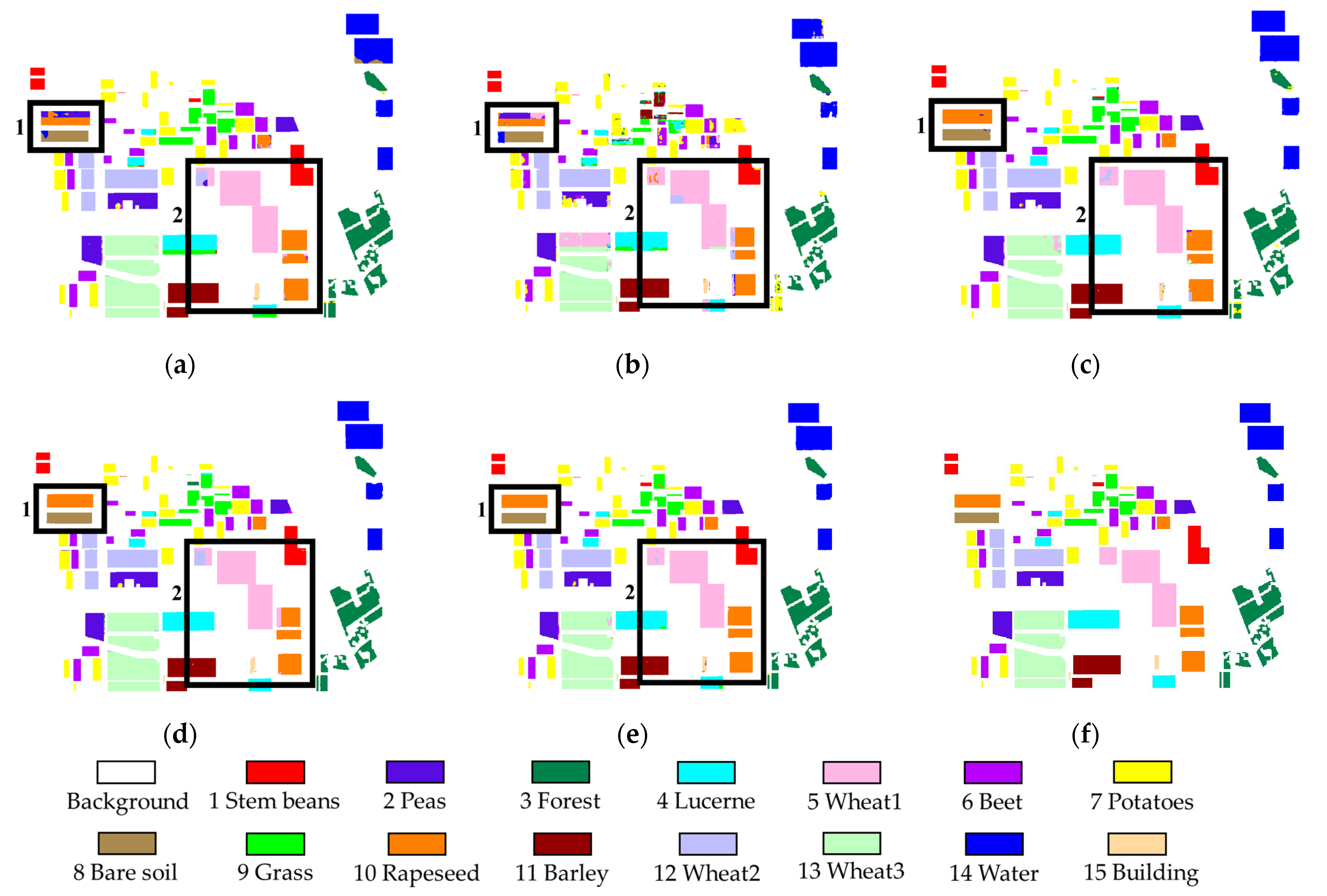
The semantic segmentation results of the Flevoland dataset obtained by five networks are shown in Figure 7a–e. Figure 7f gives the ground truth. Comparing the segmentation results of CV networks with those of RV networks, we can find that the results shown in Figure 7c–e are better than those shown in Figure 7a,b, especially in the black box area marked with the number 1. In this area, rapeseed is seriously misclassified into pea, wheat1, wheat2 and wheat3 by two RV networks, because the scattering mechanisms of these land covers are close. For bare soil in this area, since its scattering mechanism is close to that of water, it is misclassified into water by two RV networks. However, this situation is improved by three CV networks. Therefore, the three CV networks have a stronger ability to distinguish land covers with similar scattering mechanisms than two RV networks, because CV networks can extract abundant information from CV data.

For the black box area marked with the number 2 shown in Figure 7a–e, we enlarge them to obtain Figure 8a–e, respectively. The enlarged ground truth and Pauli RGB image of this area are given in Figure 8f,g, respectively. From Figure 8a to Figure 8e, wheat1 has different degrees of incorrect segmentation, because its scattering mechanism is very close to that of wheat2 and wheat3. However, the error area for wheat1 in Figure 8e is much smaller than that in the other figures, which means that the proposed network has stronger discrimination ability on land covers with similar scattering mechanisms than other networks. Similarly, the rapeseed in this area is wrongly classified by all the networks except by the proposed network.

To quantitatively analyze the segmentation performance, we calculated four indicators, and they are shown in

Table 2. Four indicators of Flevoland dataset.

Class	U-Net	DeepLabv3+	CV U-Net	L-CV-DeepLabv3+	Proposed
1	97.52	88.04	92.33	89.07	98.58
2	74.24	30.40	92.04	90.82	92.97
3	98.22	65.00	88.83	93.47	99.47
4	67.43	53.30	97.99	95.84	93.26
5	85.47	45.20	88.05	82.18	95.88
6	96.15	71.85	97.79	97.07	98.14
7	96.36	51.07	88.96	96.75	98.51
8	62.51	62.68	96.98	93.84	99.70
9	64.86	11.65	97.05	94.48	89.10
10	75.15	30.33	91.52	90.03	98.02
11	99.96	71.09	99.25	99.18	99.42
12	79.20	67.85	82.58	78.08	98.64
13	99.35	72.97	96.31	98.98	98.91
14	86.80	82.90	97.76	94.78	96.08
15	92.70	62.63	83.97	80.43	88.63
MIOU	85.99	60.32	93.20	92.13	96.57
OA	97.65	90.39	98.80	98.52	99.43
MPA	93.37	73.14	96.62	96.11	98.22

. It is easy to find that three CV networks achieve higher MIOUs, OAs and MPAs than two RV networks. In addition, the proposed network achieves the highest MIOU, OA and MPA among all the networks. Comparing the proposed network with CV U-Net, we can find that the embedded capsule network increases MIOU, OA and MPA by 3.37%, 0.63% and 1.6%, respectively, and increases IOUs of wheat1, wheat2, and wheat3 by 7.83%, 16.06%, and 2.6%, respectively. Comparing CV U-Net with L-CV-DeepLabv3+, their MIOUs, OAs and MPAs are very close to each other, which means that they have similar feature extraction ability on this dataset.

4.3.2. Experiments on San Francisco Dataset

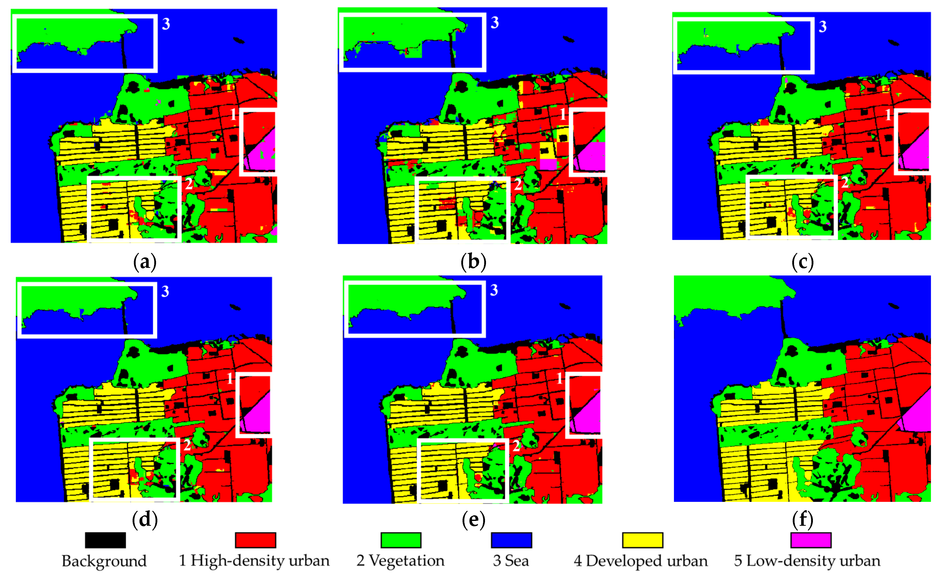
The experimental results of the San Francisco dataset obtained by five networks are shown in Figure 9a–e. Figure 9f shows the ground truth. In the white box area marked with the number 1, the part of low density is misclassified into vegetation by two RV networks because of their similar scattering mechanism. However, the segmentation results obtained by three CV networks in this area are significantly better than those obtained by two RV networks. A similar situation occurs in the white box area marked with the number 2. The segmentation results of the developed urban area obtained by two RV networks are worse than those obtained by three CV networks.

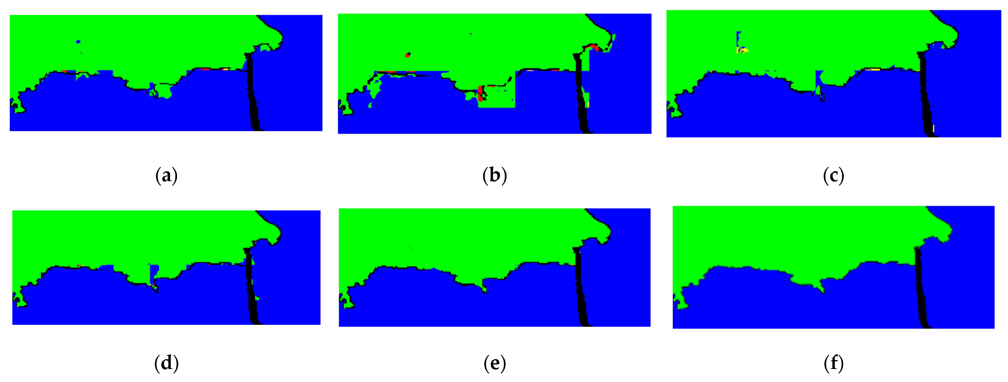
For the white box area marked with the number 3 shown in Figure 9a–e, they are magnified as Figure 10a–e, respectively. The enlarged ground truth of this area is given in Figure 10f. There are serious errors at the boundaries between vegetation and sea in Figure 10a,b. However, these boundaries are improved in Figure 10c,d. The boundaries shown in Figure 10e are very close to the ground truth. Thus, the proposed network has significant advantage in extracting the boundary information. The reason is that the embedded CV capsule network has a strong ability to extract features of land covers.

Four indicators are also calculated to quantitatively analyze the segmentation performance, and they are shown in

Table 3. Four indicators of San Francisco dataset.

Class	U-Net	DeepLabv3+	CV U-Net	L-CV-DeepLabv3+	Proposed
1	88.95	72.24	92.15	94.13	96.76
2	87.55	77.13	94.21	94.23	97.53
3	98.18	96.14	99.08	99.05	99.83
4	88.75	68.63	90.34	93.43	96.06
5	70.35	45.25	87.06	96.08	91.46
MIOU	88.96	74.72	93.80	95.86	96.93
OA	96.57	90.89	97.93	98.24	99.18
MPA	93.60	85.17	96.83	97.80	98.74

. It is obvious that three CV networks achieve higher IOUs, MIOUs, OAs and MPAs than two RV networks. Furthermore, the proposed network achieves the highest MIOU, OA and MPA among all the networks. Comparing the proposed network with CV U-Net, we can find that the embedded capsule network increases MIOU, OA and MPA by 3.13%, 1.25% and 1.91%, respectively, and increases IOUs of high-density urban and developed urban areas by 4.61% and 5.72%, respectively. Different from the previous dataset, L-CV-DeepLabv3+ achieves higher MIOU, OA and MPA than CV U-Net. This is because there are more boundaries between different categories in this dataset than in the previous dataset, and the boundary extraction ability of L-CV-DeepLabv3+ is better than that of CV U-Net.

4.3.3. Experiments on Hulunbuir Dataset

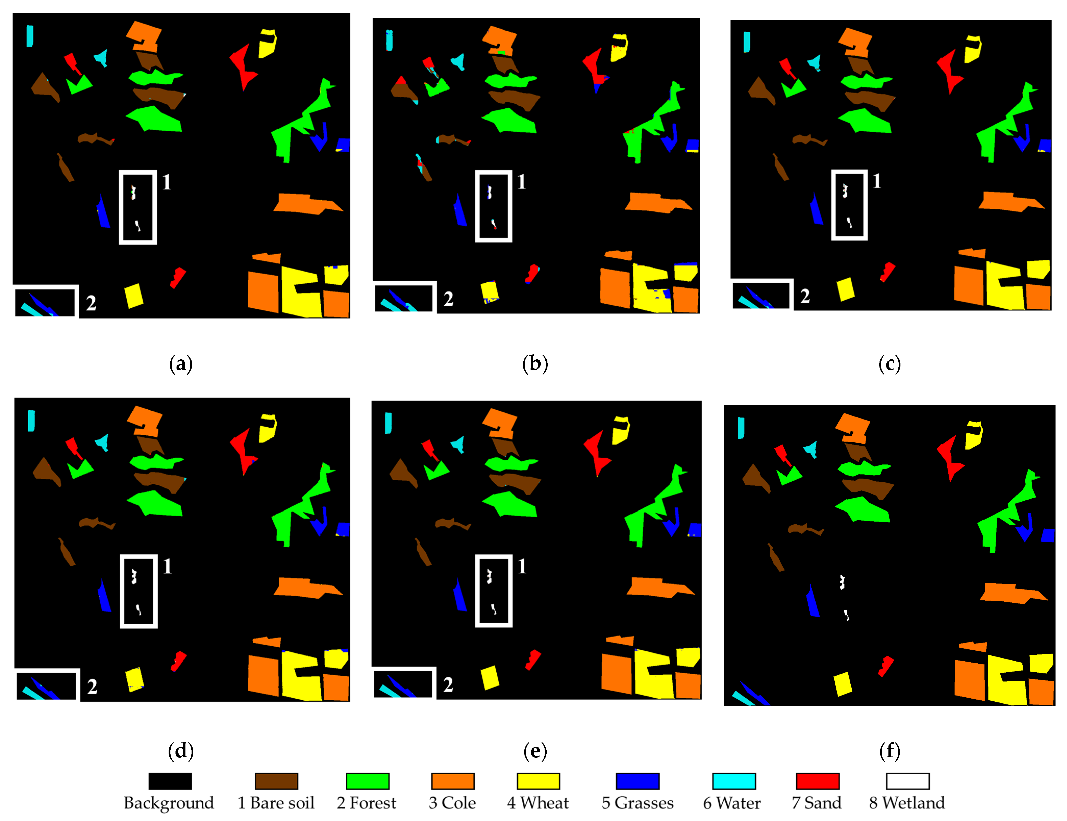
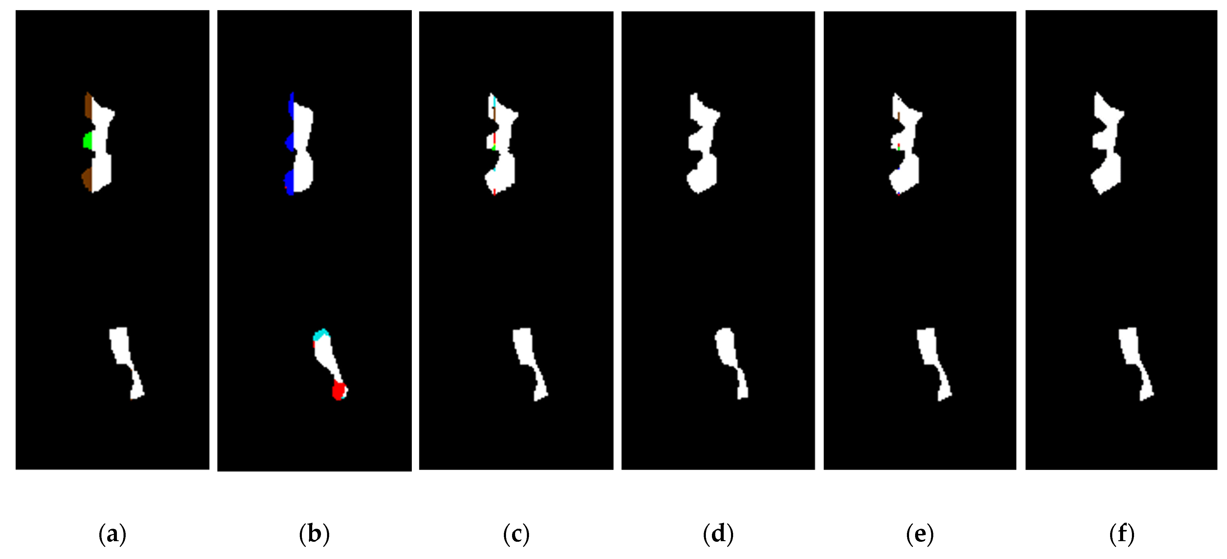
The experimental results of the Hulunbuir dataset obtained by five networks are shown in Figure 11a–e. Figure 11f shows the ground truth. In this dataset, the area ratio of land cover to the total area is small, and the intervals between different land covers are wide. This enables all the networks except for DeepLabv3+ to achieve good segmentation results. In the white box area marked with the number 1, there is only wetland. We enlarged this area in Figure 11a–e to obtain Figure 12a–e, respectively. The enlarged ground truth of this area is shown in Figure 12f. It is easy to find that there are some errors in the boundaries of segmentation results obtained by two RV networks. However, three CV networks greatly improve this situation. In the white box area marked with the number 2, there are water and grasses. We enlarged this area in Figure 11a–e to obtain Figure 13a–e, respectively. The enlarged ground truth and Pauli RGB image of this area are shown in Figure 13f–g, respectively. We can see that grasses are seriously misclassified as water by DeepLabv3+ because of their similar scattering mechanisms. Furthermore, there are some errors at the boundaries obtained by CV U-Net and L-CV-DeepLabv3+. However, the proposed network achieves boundaries that are almost close to the ground truth.

Four indicators obtained by each network are shown in

Table 4. Four indicators of Hulunbuir dataset.

Class	U-Net	DeepLabv3+	CV U-Net	L-CV-DeepLabv3+	Proposed
1	96.41	70.26	98.80	96.14	99.16
2	99.27	91.17	99.69	97.93	99.94
3	99.68	93.43	99.86	98.53	99.97
4	96.00	74.76	97.73	93.91	97.97
5	85.10	31.55	89.82	78.09	92.94
6	87.66	34.31	86.30	88.50	95.30
7	94.70	3.38	94.91	88.20	95.97
8	56.03	36.12	90.32	88.56	96.48
MIOU	90.53	59.29	95.27	92.15	97.53
OA	99.64	96.23	99.80	99.27	99.87
MPA	94.09	71.33	97.33	95.61	98.59

. The MIOUs, OAs and MPAs obtained by all the networks except for DeepLabv3+ are more than 90%. Furthermore, the proposed network achieves the highest MIOU, OA and MPA among the five networks. It also achieves the highest IOU of each type of land cover. Especially, for the small area of the wetland, the IOU obtained by the proposed network is 40.45%, 60.36%, 6.16% and 7.92% higher than that of U-Net, DeepLabv3+, CV U-Net and L-CV-DeepLabv3+, respectively. Comparing the proposed network with CV U-Net, we can find that the embedded capsule network increases MIOU, OA and MPA by 2.26%, 0.07% and 1.26%, respectively, and increases IOUs of grasses and water by 3.12% and 9%, respectively. In addition, CV U-Net achieves higher MIOU, OA and MPA than L-CV-DeepLabv3+. Therefore, based on the results of the three datasets, we can conclude that CV U-Net is more suitable for the simple dataset than L-CV-DeepLabv3+.

4.3.4. Parameters and Training Time

Since the network structure adopted by the three datasets is the same except for the number of categories, we take the Flevoland dataset as an example to analyze the parameters of five networks. The trainable, non-trainable and total parameters of the five networks are listed in

Table 5. Parameters of five networks for Flevoland dataset.

Parameter	U-Net	DeepLabv3+	CV U-Net	L-CV-DeepLabv3+	Proposed
Trainable	1,466,380	3,011,789	2,934,366	8,361,528	3,411,760
Non-trainable	3212	41,724	8030	144,620	8080
Total	1,469,592	3,053,513	2,942,396	8,506,148	3,419,840

. We can find that the parameters of CV U-Net are almost twice those of U-Net, because a CV number refers to both real and imagery parts. Similarly, the total parameters of L-CV-DeepLabv3+ are approximately 2.8 times of those of DeepLabv3+. Although the total parameters of the proposed network are more than those of CV U-Net, they are far less than those of L-CV-DeepLabv3+.

Furthermore, we compare the training time of three CV networks and list the average training time of one epoch for the three datasets in

Table 6. Average training time of one epoch for three datasets (s).

Dataset	CV U-Net	L-CV-DeepLabv3+	Proposed
Flevoland dataset	9.28	29.81	9.68
San Francisco dataset	12.98	35.59	16.5
Hulunbuir dataset	9.44	32.68	10.76

. For each dataset, the proposed network only takes a little more time than CV U-Net, but much less time than L-CV-DeepLabv3+.

4.3.5. Convergence Performance

We compared the convergence performance of the proposed network and CV U-Net. The training loss curves of the three datasets are shown in Figure 14a–c. When these two networks converge, the consumed epochs are listed in

Table 7. Epochs consumed by the convergence for three datasets (epochs).

Dataset	CV U-Net	Proposed
Flevoland dataset	540 538 527	445
San Francisco dataset		308
Hulunbuir dataset		397

. Here, we define the convergence as the loss difference between two adjacent epochs that does not exceed 0.003 for five consecutive times. For each dataset, the proposed network consumes less epochs than CV U-Net. Therefore, it can be inferred from Table 6 and Table 7 that the convergence speed of the proposed network is much faster than that of CV U-Net for each dataset.

5. Discussion

From the experimental results in Section 4, we know that the proposed network has significant advantages over the other four networks. In this section, we discuss the influence of training set size on segmentation performance of the proposed network and CV U-Net, and we analyze advantages of the embedded CV capsule network in feature extraction through the visualization of feature maps.

5.1. Influence of Training Set Size on Segmentation Performance

We compare the segmentation performance of the proposed network and CV U-Net when the expansion factor of the training samples changes. The curves of segmentation performance for the three datasets are shown in Figure 15a–c. When the training set is not expanded, the segmentation performance of the proposed network is far better than that of CV U-Net for each dataset. For the Flevoland dataset, the MIOU difference between these two networks is greater than 16%, and the MPA difference is greater than 10%. For the San Francisco dataset, these two differences are greater than 29% and 20%, respectively. For the Hulunbuir dataset, these two differences are greater than 25% and 17%, respectively. Furthermore, for the three datasets, the MIOUs obtained by the proposed network are equal to or greater than 90%. Therefore, the proposed network has significant advantages when the training sets are not expanded.

As the training samples increase, the segmentation performances obtained by these two networks are gradually improved for each dataset. This is because more features can be extracted from the expanded training samples. At the same time, we can find that the performance difference between these two networks gradually decreases for each dataset. However, the proposed network achieves higher MIOU, OA and MPA than CV U-Net, regardless of the expansion factor of training samples. In addition, we can also find that no matter the CV U-Net or proposed network, the OA obtained is the largest, followed by MPA, and finally MIOU. The reason is that the MIOU is stricter than the other two indicators.

5.2. Advantages of the Capsule Network in Feature Extraction

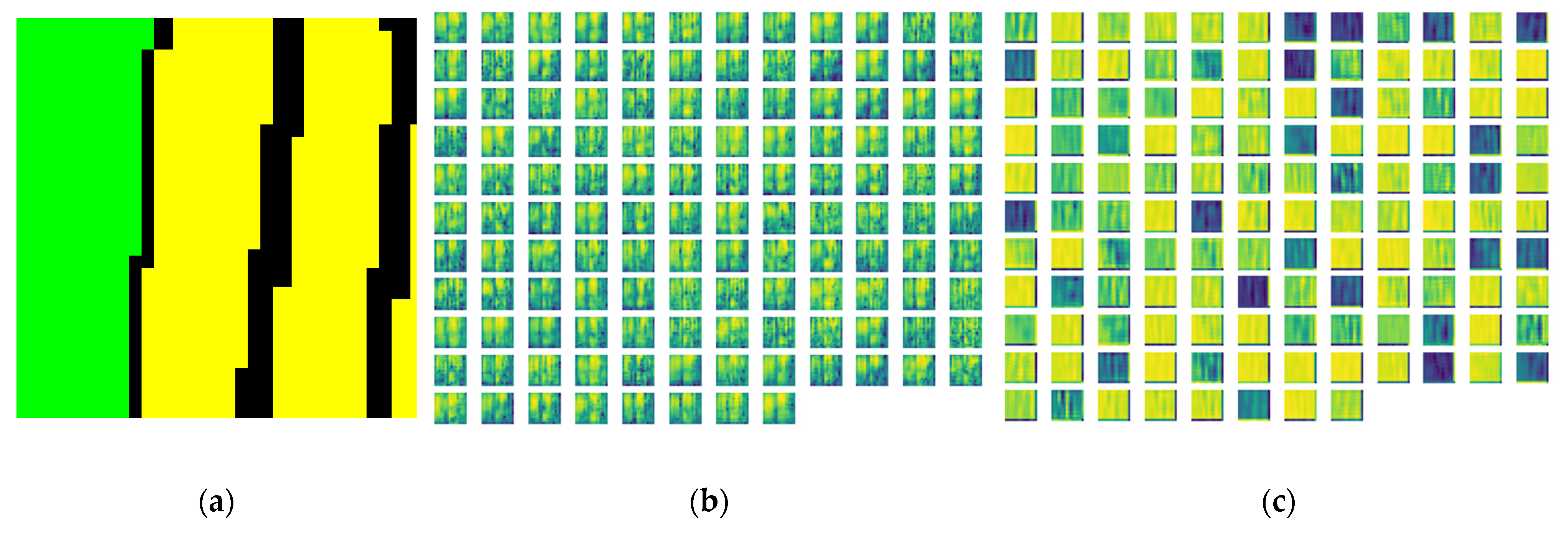
To demonstrate the feature extraction ability of the embedded capsule network, we visualize the feature maps obtained by the proposed network and CV U-Net. For the proposed network shown in Figure 4, feature maps (in the red box) obtained after the first upsampling and convolution operation are considered. For CV U-Net, feature maps obtained at the corresponding position are also considered. Taking the San Francisco dataset as an example, the ground truth of one test sample is shown in Figure 16a. When the number of training samples is not expanded, the visualization results of 128 feature maps obtained by the proposed network are shown in Figure 16c. The feature maps at the corresponding position obtained by CV U-Net are shown in Figure 16b. Comparing Figure 16b with Figure 16c, we can find that the texture features in Figure 16c are clearer than those in Figure 16b. The former is the global features. Therefore, the embedded CV capsule network enhances the feature extraction ability of CV U-Net.

6. Conclusions

In this paper, we propose a CV U-Net with a capsule embedded for semantic segmentation of PolSAR images. The proposed network mainly includes two parts. One is the CV U-Net, and the other is the CV capsule network. The CV U-Net is obtained by extending the original U-Net to the CV domain and making its structure lightweight. Like the original U-Net, it also includes the encoder and the decoder. The CV capsule network is embedded between the CV encoder and the CV decoder. It is made up of the CV primary capsule and the segmented capsule. In order to accomplish the connection between these two types of capsules, CV dynamic routing is proposed. It can ensure the routing consistency of real and imaginary parts of CV capsules. From the experimental results for two airborne datasets and one spaceborne dataset, we can draw the following conclusions: (1) CV networks have better performance than RV networks because the former can make full use of both the amplitude and phase information of PolSAR data. (2) The structure of the network should match the dataset to achieve good performance. The reason is that overfitting can easily occur when a small number of samples are used for the training of a deep network. (3) The proposed network can not only effectively distinguish land covers with the similar scattering mechanism, but it can also obtain the accurate boundaries of land covers. These advantages are especially obvious when the number of training samples is small. The reason is that the embedded CV capsule network has a strong ability of feature extraction.

References

1. Lee, J.S.; Pottier, E. Polarimetric Radar Imaging: From Basics to Applications; CRC Press: Boca Raton, FL, USA, 2009. [Google Scholar]
2. Cloude, S.R.; Pottier, E. An entropy based classification scheme for land applications of polarimetric SAR. IEEE Trans. Geosci. Remote Sens. 1997, 35, 68–78. [Google Scholar] [CrossRef]
3. Lee, J.S.; Grunes, M.R.; Ainsworth, T.L.; Du, L.J.; Schuler, D.L.; Cloude, S.R. Unsupervised classification using polarimetric decomposition and the complex Wishart classifier. IEEE Trans. Geosci. Remote Sens. 1991, 37, 2249–2258. [Google Scholar]
4. Jiao, L.; Liu, F. Wishart deep stacking network for fast PolSAR image classification. IEEE Trans. Image Process. 2016, 25, 3273–3286. [Google Scholar] [CrossRef]
5. Zhang, Z.; Wang, H.; Xu, F.; Jin, Y.Q. Complex-valued convolutional neural network and its application in polarimetric SAR image classification. IEEE Trans. Geosci. Remote Sens. 2017, 55, 7177–7188. [Google Scholar] [CrossRef]
6. Cheng, J.; Zhang, F.; Xiang, D.; Yin, Q.; Zhou, Y. PolSAR image classification with multiscale superpixel-based graph convolutional network. IEEE Trans. Geosci. Remote Sens. 2022, 60, 1–14. [Google Scholar] [CrossRef]
7. Dong, H.; Zou, B.; Zhang, L.; Zhang, S. Automatic design of CNNs via differentiable neural architecture search for PolSAR image classification. IEEE Trans. Geosci. Remote Sens. 2020, 58, 6362–6375. [Google Scholar] [CrossRef] [Green Version]
8. Liu, H.; Yang, S.; Gou, S.; Chen, P.; Wang, Y.; Jiao, L. Fast classifiction for large polarimeteric SAR data based on refined spatial-anchor graph. IEEE Geosci. Remote Sens. Lett. 2017, 14, 1589–1593. [Google Scholar] [CrossRef]
9. Ding, L.; Zheng, K.; Lin, D.; Chen, Y.; Bruzzone, L. MP-ResNet: Multipath residual network for the semantic segmentation of high-resolution PolSAR images. IEEE Geosci. Remote. Sens. Lett. 2022, 19, 4014205. [Google Scholar] [CrossRef]
10. Xiao, D.; Wang, Z.; Wu, Y.; Gao, X.; Sun, X. Terrain segmentation in polarimetric SAR images using dual-attention fusion network. IEEE Geosci. Remote Sens. Lett. 2022, 19, 4006005. [Google Scholar] [CrossRef]
11. Garg, R.; Kumar, A.; Bansal, N.; Prateek, M.; Kumar, S. Semantic segmentation of PolSAR image data using advanced deep learning model. Sci. Rep. 2021, 11, 15365. [Google Scholar] [CrossRef]
12. Ren, S.; Zhou, F. Semi-supervised classification for PolSAR data with multi-scale evolving weighted graph convolutional network. IEEE J. Sel. Top. Appl. Earth Observ. Remote Sens. 2021, 14, 2911–2927. [Google Scholar] [CrossRef]
13. Chen, S.W.; Tao, C.S. PolSAR image classification using polarimetric-feature-driven deep convolutional neural network. IEEE Geosci. Remote Sens. Lett. 2018, 15, 627–631. [Google Scholar] [CrossRef]
14. Ni, J.; Zhang, F.; Yin, Q.; Zhou, Y.; Li, H.-C.; Hong, W. Random neighbor pixel-block-based deep recurrent learning for polarimetric SAR image classification. IEEE Trans. Geosci. Remote Sens. 2021, 59, 7557–7569. [Google Scholar] [CrossRef]
15. Liu, F.; Jiao, L.; Hou, B.; Yang, S. POL-SAR image classification based on Wishart DBN and local spatial information. IEEE Trans. Geosci. Remote Sens. 2016, 54, 3292–3308. [Google Scholar] [CrossRef]
16. Xie, W.; Jiao, L.; Hou, B.; Ma, W.; Zhao, J.; Zhang, S.; Liu, F. PolSAR image classification via Wishart-AE model or Wishart-CAE model. IEEE J. Sel. Top. Appl. Earth Observ. Remote Sens. 2017, 10, 3604–3615. [Google Scholar] [CrossRef]
17. Liu, F.; Jiao, L.; Tang, X. Task-oriented GAN for PolSAR image classification and clustering. IEEE Trans. Neural Netw. Learn. Syst. 2019, 30, 2707–2719. [Google Scholar] [CrossRef]
18. Fang, Z.; Zhang, G.; Dai, Q.; Kong, Y.; Wang, P. Semisupervised deep convolutional neural networks using pseudo labels for PolSAR image classification. IEEE Geosci. Remote Sens. Lett. 2022, 19, 4005605. [Google Scholar] [CrossRef]
19. Liu, H.; Xu, D.; Zhu, T.; Shang, F.; Yang, R. Graph convolutional networks by architecture search for PolSAR image classification. Remote Sens. 2021, 13, 1404. [Google Scholar] [CrossRef]
20. Bi, H.; Sun, J.; Xu, Z. A graph-based semisupervised deep learning model for PolSAR image classification. IEEE Trans. Geosci. Remote Sens. 2018, 57, 2116–2132. [Google Scholar] [CrossRef]
21. Liu, S.J.; Luo, H.; Shi, Q. Active ensemble deep learning for polarimetric synthetic apetrue radar image classification. IEEE Geosci. Remote Sens. Lett. 2021, 18, 1580–1584. [Google Scholar] [CrossRef]
22. Bi, H.; Xu, F.; Wei, Z.; Xue, Y.; Xu, Z. An active deep learning approach for minimally supervised PolSAR image classification. IEEE Trans. Geosci. Remote Sens. 2019, 57, 9378–9395. [Google Scholar] [CrossRef]
23. Zhou, Y.; Wang, H.; Xu, F.; Jin, Y.Q. Polarimetric SAR image classification using deep convolutional neural networks. IEEE Geosci. Remote Sens. Lett. 2016, 13, 1935–1939. [Google Scholar] [CrossRef]
24. Gao, F.; Huang, T.; Wang, J.; Sun, J.P.; Hussain, A.; Yang, E. Dual-branch deep convolution neural network for polarimetric SAR image classification. Appl. Sci. 2017, 7, 447. [Google Scholar] [CrossRef] [Green Version]
25. Wang, Y.; Chen, J.; Zhou, Y.; Zhang, F.; Yin, Q. A multi-channel fusion convolution neural network based on scattering mechanism for PolSAR image classification. IEEE Geosci. Remote Sens. Lett. 2022, 19, 4007805. [Google Scholar]
26. Dong, H.; Zhang, L.; Zou, A.B. PolSAR image classification with lightweight 3D convolutional networks. Remote Sens. 2020, 12, 396. [Google Scholar] [CrossRef] [Green Version]
27. Liu, X.; Jiao, L.; Tang, X.; Sun, Q.; Zhang, D. Polarimetric convolutional network for PolSAR image classification. IEEE Trans. Geosc. Remote Sens. 2019, 57, 3040–3054. [Google Scholar] [CrossRef] [Green Version]
28. Zhang, L.; Dong, H.; Zou, B. Efficently utilizing complex-valued PolSAR image data via a multi-task deep learning framework. ISPRS J. Photogramm. Remote Sens. 2019, 157, 59–72. [Google Scholar] [CrossRef] [Green Version]
29. Tan, X.; Li, M.; Zhang, P.; Wu, Y.; Song, W. Complex-valued 3D convolutional neural network for PolSAR image classification. IEEE Geosci. Remote Sens. Lett. 2020, 17, 1022–1026. [Google Scholar] [CrossRef]
30. Zhang, P.; Tan, X.; Li, B.; Jiang, Y.; Wu, Y. PolSAR image classification using hybrid conditional random fields model based on complex-valued 3D CNN. IEEE Trans. Aerosp. Electron. Syst. 2021, 57, 1713–1730. [Google Scholar] [CrossRef]
31. Xie, W.; Ma, G.; Zhao, F.; Zhang, L. PolSAR image classification via a novel semi-supervised recurrent complex-valued convolution neural network. Neurocomputing 2020, 388, 255–268. [Google Scholar] [CrossRef]
32. Long, J.; Shelhamer, E.; Darrell, T. Fully convolutional networks for semantic segmentation. In Proceedings of the 2015 IEEE Conference on Computer Vision and Pattern Recognition, Boston, MA, USA, 7–12 June 2015; pp. 3431–3440. [Google Scholar]
33. Ronneberger, O.; Fischer, P.; Brox, T. U-net: Convolutional networks for biomedical image segmentation. In Proceedings of the 18th International Conference on Medical Image Computing and Computer Assisted Interventions, Munich, Germany, 5–9 October 2015; pp. 234–241. [Google Scholar]
34. Badrinarayanan, V.; Kendall, A.; Cipolla, R. Segnet: A deep convolutional encoder-decoder architecture for image segmentation. IEEE Trans. Pattern Anal. Mach. Intell. 2017, 39, 2481–2495. [Google Scholar] [CrossRef] [PubMed]
35. Zhao, H.; Shi, J.; Qi, X.; Wang, X.; Jia, J. Pyramid scene parsing network. In Proceedings of the IEEE Conference on Computer Vision and Pattern Recognition, Honolulu, HI, USA, 21–26 July 2017; pp. 6230–6239. [Google Scholar]
36. Chen, L.C.; Zhu, Y.; Papandreou, G.; Schroff, F.; Adam, H. Encoder-decoder with atrous separable convolution for semantic image segmentation. In Proceedings of the 2018 European Conference on Computer Vision (ECCV), Munich, Germany, 8–14 September 2018; pp. 801–818. [Google Scholar]
37. Lin, G.; Milan, A.; Shen, C.; Reid, I. RefineNet: Multi-path refinement networks for high-resolution semantic segmentation. In Proceedings of the IEEE Conference on Computer Vision and Pattern Recognition, Honolulu, HI, USA, 21–26 July 2017; pp. 5168–5177. [Google Scholar]
38. Sun, X.; Shi, A.; Huang, H.; Mayer, H. BAS4NET: Boundary-aware semi-supervised semantic segmentation network for very high resolution remote sensing images. IEEE J. Sel. Top. Appl. Earth Observ. Remote Sens. 2020, 13, 5398–5413. [Google Scholar] [CrossRef]
39. Shahzad, M.; Maurer, M.; Fraundorfer, F.; Wang, Y.; Zhu, X.X. Buildings detection in VHR SAR images using fully convolution neural networks. IEEE Trans. Geosci. Remote Sens. 2019, 57, 1100–1116. [Google Scholar] [CrossRef] [Green Version]
40. Shi, X.; Fu, S.; Chen, J.; Wang, F.; Xu, F. Object-level semantic segmentation on the high-resolution Gaofen-3 FUSAR-map dataset. IEEE J. Sel. Top. Appl. Earth Observ. Remote Sens. 2021, 14, 3107–3119. [Google Scholar] [CrossRef]
41. Bianchi, F.M.; Grahn, J.; Eckerstorfer, M.; Malnes, E.; Vickers, H. Snow avalanche segmentation in SAR images with fully convolutional neural networks. IEEE J. Sel. Top. Appl. Earth Observ. Remote Sens. 2021, 14, 75–82. [Google Scholar] [CrossRef]
42. Wang, Y.; He, C.; Liu, X.L.; Liao, M.S. A hierarchical fully convolutional network integrated with sparse and low-rank subspace representations for PolSAR imagery classification. Remote Sens. 2018, 10, 342. [Google Scholar] [CrossRef] [Green Version]
43. He, C.; He, B.; Tu, M.; Wang, Y.; Qu, T.; Wang, D.; Liao, M. Fully convolutional networks and a manifold graph embedding-based algorithm for PolSAR image classification. Remote Sens. 2020, 12, 1467. [Google Scholar] [CrossRef]
44. Li, Y.; Chen, Y.; Liu, G.; Jiao, L. A novel deep fully convolutional network for PolSAR image classification. Remote Sens. 2018, 10, 1984. [Google Scholar] [CrossRef] [Green Version]
45. Mohammadimanesh, F.; Salehi, B.; Mandianpari, M.; Gill, E.; Molinier, M. A new fully convolutional neural network for semantic segmentation of polarimetric SAR imagery in complex land cover ecosystem. ISPRS J. Photogramm. Remote Sens. 2019, 151, 223–236. [Google Scholar] [CrossRef]
46. Pham, M.T.; Lefèvre, S. Very high resolution airborne PolSAR image classification using convolutional neural networks. arXiv 2019, arXiv:1910.14578. [Google Scholar]
47. Wu, W.; Li, H.; Li, X.; Guo, H.; Zhang, L. PolSAR image semantic segmentation based on deep transfer learning-realizing smooth classification with small training sets. IEEE Geosci. Remote Sens. Lett. 2019, 19, 977–981. [Google Scholar] [CrossRef]
48. Zhao, F.; Tian, M.; Wen, X.; Liu, H. A new parallel dual-channel fully convolutional network via semi-supervised fcm for PolSAR image classification. IEEE J. Sel. Top. Appl. Earth Observ. Remote Sens. 2020, 13, 4493–4505. [Google Scholar] [CrossRef]
49. Jing, H.; Wang, Z.; Sun, X.; Xiao, D.; Fu, K. PSRN: Polarimetric space reconstruction network for PolSAR image semantic segmentation. IEEE J. Sel. Top. Appl. Earth Observ. Remote Sens. 2021, 14, 10716–10732. [Google Scholar] [CrossRef]
50. Cao, Y.; Wu, Y.; Zhang, P.; Liang, W.; Li, M. Pixel-wise PolSAR image classification via a novel complex-valued deep fully convolutional network. Remote Sens. 2019, 11, 2653. [Google Scholar] [CrossRef] [Green Version]
51. Yu, L.; Zeng, Z.; Liu, A.; Xie, X.; Wang, H.; Xu, F.; Hong, W. A lightweight complex-valued DeepLabv3+ for semantic segmentation of PolSAR image. IEEE J. Sel. Top. Appl. Earth Observ. Remote Sens. 2022, 15, 930–943. [Google Scholar] [CrossRef]
52. Sabour, S.; Frosst, N.; Hinton, G.E. Dynamic routing between capsules. arXiv 2017, arXiv:1710.09829. [Google Scholar]
53. Xiang, C.; Lu, Z.; Zou, W.; Yi, T.; Chen, X. Ms-CapsNet: A novel multi-scale capsule network. IEEE Signal Process. Lett. 2018, 25, 1850–1854. [Google Scholar] [CrossRef]
54. Jaiswal, A.; AbdAlmageed, W.; Wu, Y.; Natarajan, P. CapsuleGAN: Generative adversarial capsule network. arXiv 2018, arXiv:1802.06167. [Google Scholar]
55. Mobiny, A.; Van Nguyen, H. Fast CapsNet for lung cancer screening. In Proceedings of the International Conference on Medical Image Computing and Computer-Assisted Intervention, Granada, Spain, 16–20 September 2018; Springer: Cham, Switzerland, 2018; pp. 741–749. [Google Scholar]
56. Afshar, P.; Plataniotis, K.N.; Mohammadi, A. Capsule networks for brain tumor classification based on MRI images and coarse tumor boundaries. In Proceedings of the ICASSP 2019 IEEE International Conference on Acoustics, Speech and Signal Processing (ICASSP), Brighton, UK, 12–17 May 2019; pp. 1368–1372. [Google Scholar]
57. Zhang, W.; Tang, P.; Zhao, L. Remote sensing image scene classification using CNN-CapsNet. Remote Sens. 2019, 11, 494. [Google Scholar] [CrossRef] [Green Version]
58. Yu, Y.; Liu, C.; Guan, H.; Wang, L.; Gao, S.; Zhang, H.; Zhang, Y.; Li, J. Land cover classification of multispectral lidar data with an efficient self-attention capsule network. IEEE Geosci. Remote Sens. Lett. 2022, 19, 6501505. [Google Scholar] [CrossRef]
59. Cheng, J.; Zhang, F.; Xiang, D.; Yin, Q.; Zhou, Y.; Wang, W. PolSAR image land cover classification based on hierarchical capsule network. Remote Sens. 2021, 13, 3132. [Google Scholar] [CrossRef]
60. LaLonde, R.; Bagci, U. Capsules for object segmentation. arXiv 2018, arXiv:1804.04241. [Google Scholar]
61. Liu, A.; Yu, L.J.; Zeng, Z.X.; Xie, X.C.; Guo, Y.T.; Shao, Q.Q. Complex-valued U-Net for PolSAR image semantic segmentation. IOP J. Phys. Conf. Ser. 2021, 2010, 012102. [Google Scholar] [CrossRef]
62. Yu, L.; Hu, Y.; Xie, X.; Lin, Y.; Hong, W. Complex-valued full convolutional neural network for SAR target classification. IEEE Geosci. Remote Sens. Lett. 2020, 17, 1752–1756. [Google Scholar] [CrossRef]
Figure 1. Differences between PolSAR image classification and semantic segmentation.
Remotesensing 15 01371 g001
Figure 2. Architecture of U-Net.
Remotesensing 15 01371 g002
Figure 3. Architecture of a capsule network.
Remotesensing 15 01371 g003
Figure 4. Architecture of CV U-Net with the capsule network embedded.
Remotesensing 15 01371 g004
Figure 5. Locally constrained CV dynamic routing.
Remotesensing 15 01371 g005
Figure 6. Pauli RGB image. (a) Flevoland dataset; (b) San Francisco dataset; (c) Hulunbuir dataset.
Remotesensing 15 01371 g006
Figure 7. Segmentation results of Flevoland dataset. (a) U-Net; (b) DeepLabv3+; (c) CV U-Net; (d) L-CV-DeepLabv3+; (e) proposed network; (f) ground truth.
Remotesensing 15 01371 g007
Figure 8. Enlarged views of black box area 2 in Figure 7. (a) U-Net; (b) DeepLabv3+; (c) CV U-Net; (d) L-CV-DeepLabv3+; (e) proposed network; (f) ground truth; (g) Pauli RGB image.
Remotesensing 15 01371 g008
Figure 9. Segmentation results of San Francisco dataset. (a) U-Net; (b) DeepLabv3+; (c) CV U-Net; (d) L-CV-DeepLabv3+; (e) proposed network; (f) ground truth.
Remotesensing 15 01371 g009
Figure 10. Enlarged views of white box area 3 in Figure 9. (a) U-Net; (b) DeepLabv3+; (c) CV U-Net; (d) L-CV-DeepLabv3+; (e) proposed network; (f) ground truth.
Remotesensing 15 01371 g010
Figure 11. Segmentation results of Hulunbuir dataset. (a) U-Net; (b) DeepLabv3+; (c) CV U-Net; (d) L-CV-DeepLabv3+; (e) proposed network; (f) ground truth.
Remotesensing 15 01371 g011
Figure 12. Enlarged views of white box area 1 in Figure 11. (a) U-Net; (b) DeepLabv3+; (c) CV U-Net; (d) L-CV-DeepLabv3+; (e) proposed network; (f) ground truth.
Remotesensing 15 01371 g012
Figure 13. Enlarged views of white box area 2 in Figure 11. (a) U-Net; (b) DeepLabv3+; (c) CV U-Net; (d) L-CV-DeepLabv3+; (e) proposed network; (f) ground truth; (g) Pauli RGB image.
Remotesensing 15 01371 g013
Figure 14. Curves of training loss. (a) Flevoland dataset; (b) San Francisco dataset; (c) Hulunbuir dataset.
Remotesensing 15 01371 g014
Figure 15. Segmentation performance changes with the expansion factor of training samples. (a) Flevoland dataset; (b) San Francisco dataset; (c) Hulunbuir dataset.
Remotesensing 15 01371 g015
Figure 16. Test sample and visualization of feature maps. (a) Ground truth of the test sample; (b) feature maps obtained by CV U-Net; (c) feature maps obtained by the proposed network.
Remotesensing 15 01371 g016