
Multi-Branch Deep Neural Network for Bed Topography of Antarctica Super-Resolution: Reasonable Integration of Multiple Remote Sensing Data


Abstract
1. Introduction
2. Related Work
3. Materials and Methods
3.1. Data
3.2. Model Design
3.2.1. Direct Upsampling
3.2.2. Multi-Branch Feature Extraction
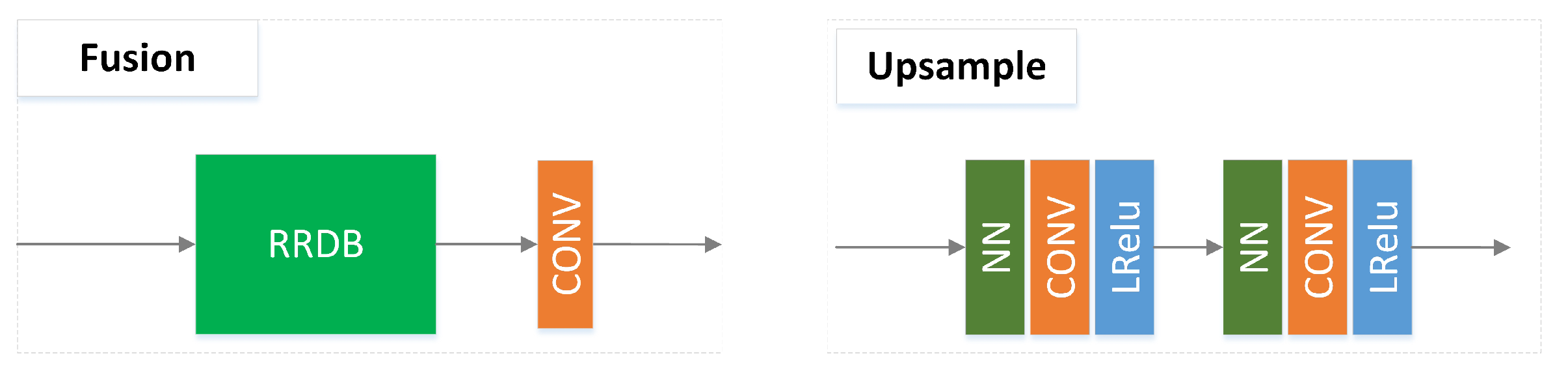
3.2.3. Upsampling with Feature Fusion
4. Results
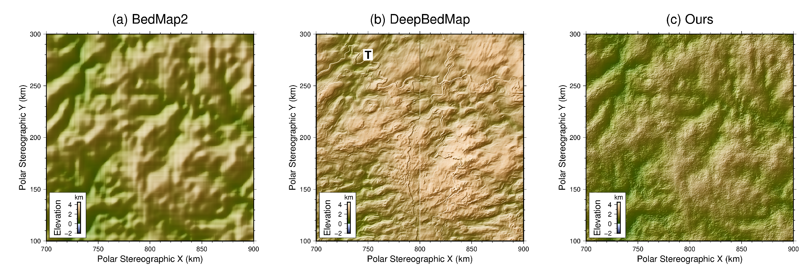
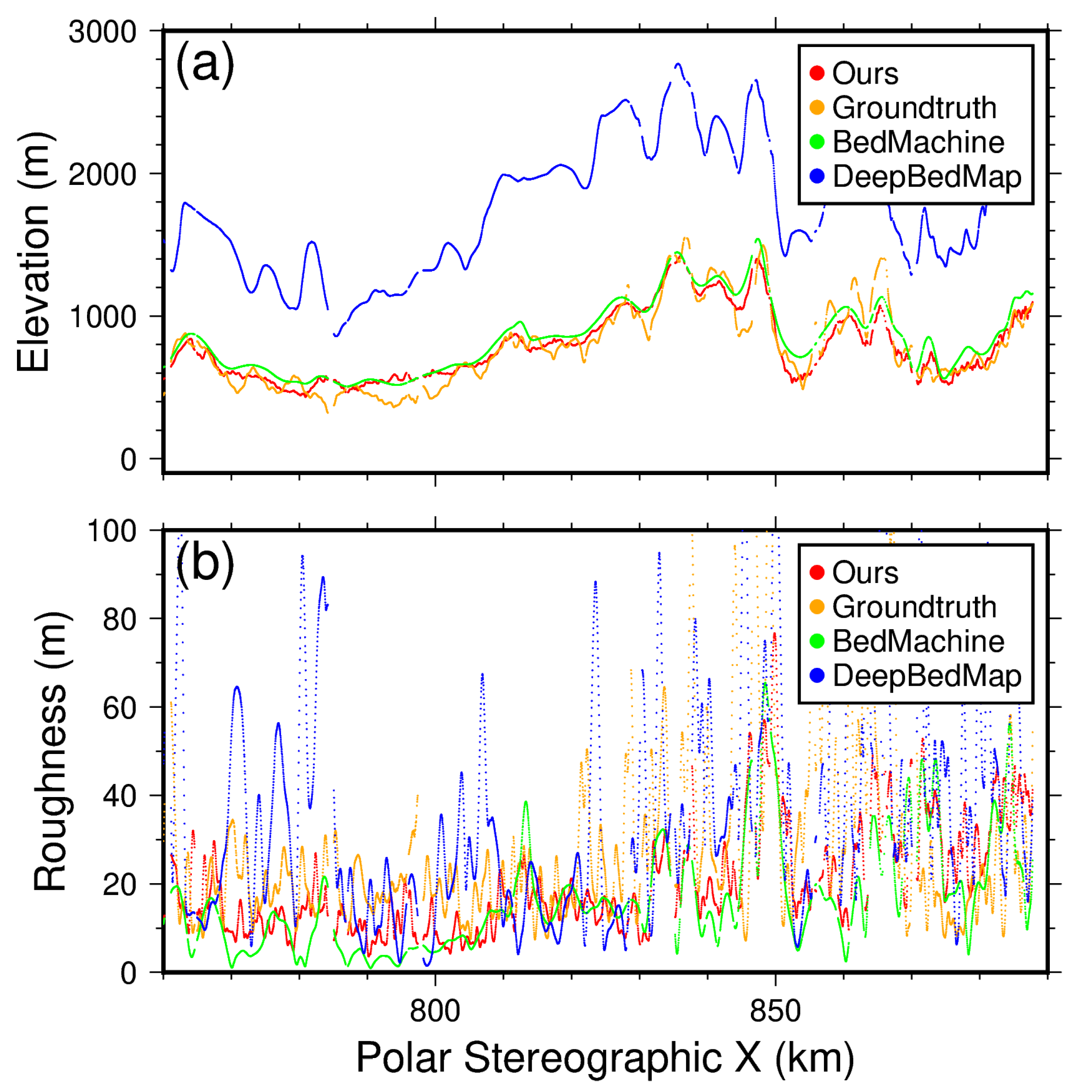
4.1. Bed Topography
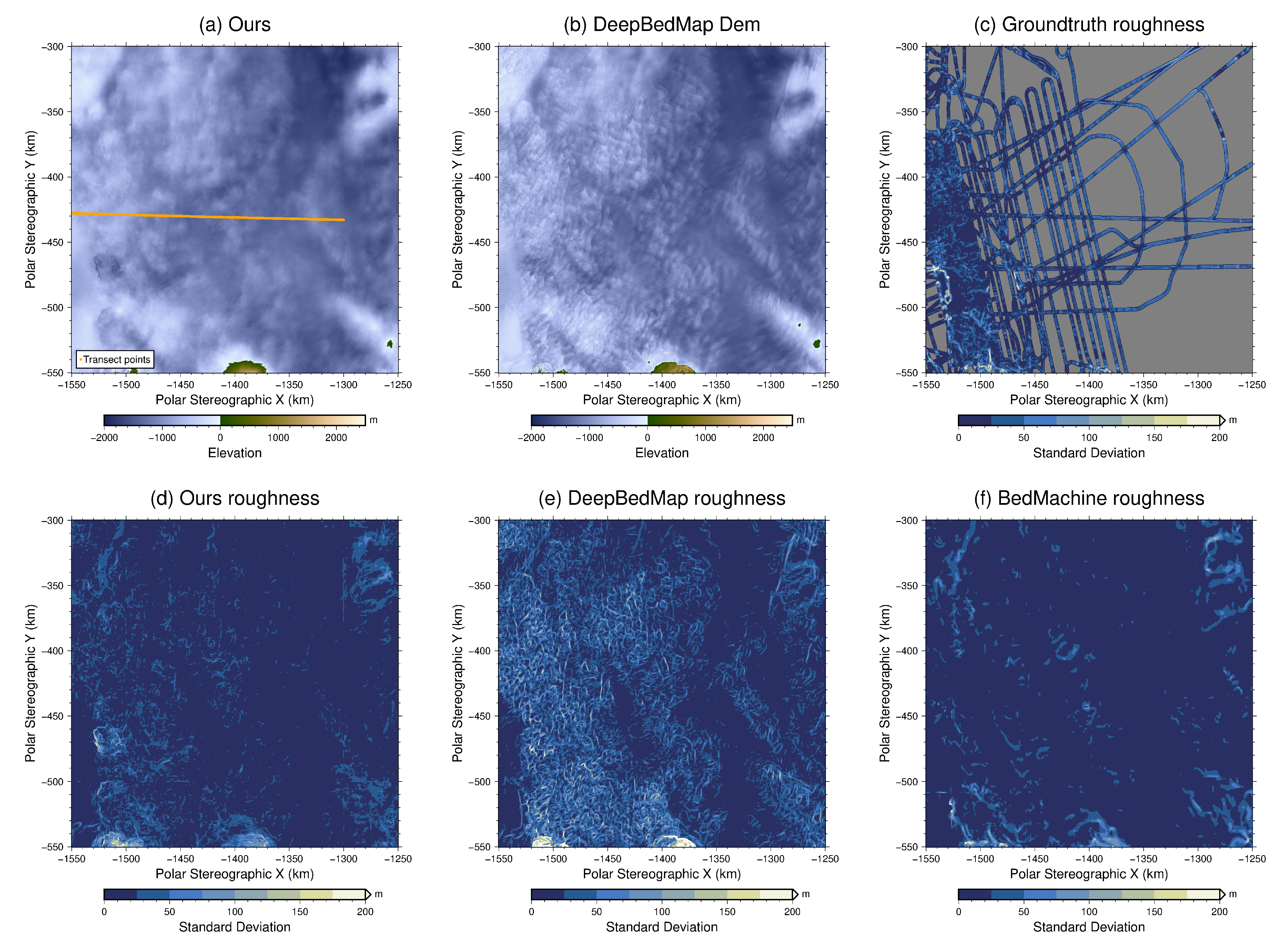
4.2. Bed Roughness
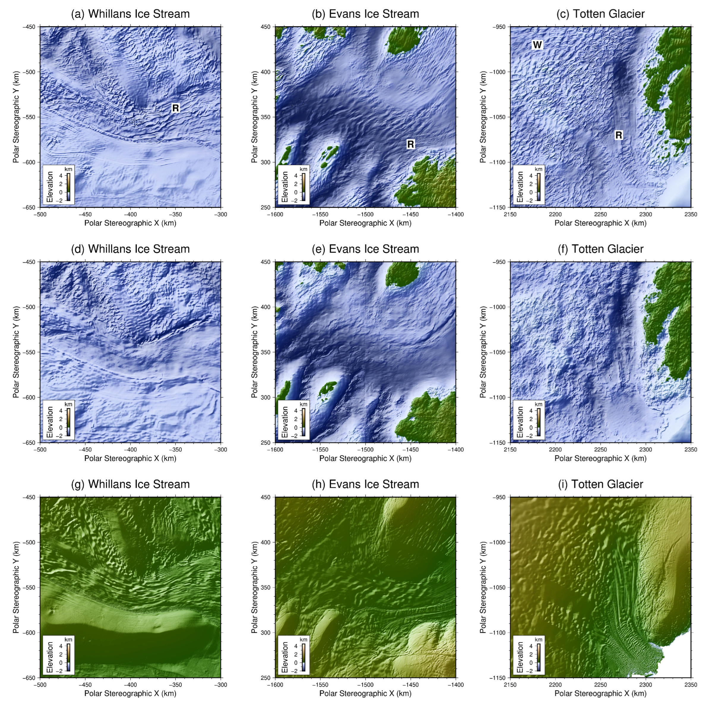
4.3. Model Generalization
4.4. Extended Experiments
5. Discussion
5.1. Bed Features
5.2. Roughness
5.3. Model Generalization
5.4. Limitations and Future Work
6. Conclusions
Author Contributions
Funding
Data Availability Statement
Conflicts of Interest
Appendix A. Deep Neural Network Training Details

| Hyperparameter | Setting | Tuning Range |
|---|---|---|
| Learning rate | to | |
| Mini-batch size | 128 | 64 or 128 |
| Number of epochs | 190 | 100 to 200 |
| Residual scaling | 0.2 | 0.1 to 0.5 |
| Adam optimizer epsilon | 0.1 | Fixed |
| Adam optimizer beta1 | 0.9 | Fixed |
| Adam optimizer beta2 | 0.99 | Fixed |
References
- Fretwell, P.; Pritchard, H.D.; Vaughan, D.G.; Bamber, J.L.; Barrand, N.E.; Bell, R.; Bianchi, C.; Bingham, R.G.; Blankenship, D.D.; Casassa, G.; et al. Bedmap2: Improved Ice Bed, Surface and Thickness Datasets for Antarctica. Cryosphere 2013, 7, 375–393. [Google Scholar] [CrossRef]
- Morlighem, M.; Rignot, E.; Binder, T.; Blankenship, D.; Drews, R.; Eagles, G.; Eisen, O.; Ferraccioli, F.; Forsberg, R.; Fretwell, P.; et al. Deep Glacial Troughs and Stabilizing Ridges Unveiled beneath the Margins of the Antarctic Ice Sheet. Nat. Geosci. 2019, 13, 132–137. [Google Scholar] [CrossRef]
- Seroussi, H.; Nakayama, Y.; Larour, E.; Menemenlis, D.; Morlighem, M.; Rignot, E.; Khazendar, A. Continued retreat of Thwaites Glacier, West Antarctica, controlled by bed topography and ocean circulation. Geophys. Res. Lett. 2017, 44, 6191–6199. [Google Scholar] [CrossRef]
- Rignot, E.; Mouginot, J.; Scheuchl, B.; Van Den Broeke, M.; Van Wessem, M.J.; Morlighem, M. Four decades of Antarctic Ice Sheet mass balance from 1979–2017. Proc. Natl. Acad. Sci. USA 2019, 116, 1095–1103. [Google Scholar] [CrossRef] [PubMed]
- Joughin, I.; Smith, B.E.; Medley, B. Marine ice sheet collapse potentially under way for the Thwaites Glacier Basin, West Antarctica. Science 2014, 344, 735–738. [Google Scholar] [CrossRef] [PubMed]
- Lythe, M.B.; Vaughan, D.G. BEDMAP: A New Ice Thickness and Subglacial Topographic Model of Antarctica. J. Geophys. Res. Solid Earth 2001, 106, 11335–11351. [Google Scholar] [CrossRef]
- Le Brocq, A.M.; Payne, A.J.; Vieli, A. An Improved Antarctic Dataset for High Resolution Numerical Ice Sheet Models (ALBMAP V1). Earth Syst. Sci. Data 2010, 2, 247–260. [Google Scholar] [CrossRef]
- Cui, X.; Jeofry, H.; Greenbaum, J.S.; Guo, J.; Li, L.; Lindzey, L.E.; Habbal, F.A.; Wei, W.; Young, D.A.; Ross, N.; et al. Bed topography of Princess Elizabeth Land in East Antarctica. Earth Syst. Sci. Data 2020, 12, 2765–2774. [Google Scholar] [CrossRef]
- Gasson, E.; DeConto, R.M.; Pollard, D.; Levy, R.H. Dynamic Antarctic ice sheet during the early to mid-Miocene. Proc. Natl. Acad. Sci. USA 2016, 113, 3459–3464. [Google Scholar] [CrossRef]
- Goff, J.A.; Powell, E.M.; Young, D.A.; Blankenship, D.D. Conditional Simulation of Thwaites Glacier (Antarctica) Bed Topography for Flow Models: Incorporating Inhomogeneous Statistics and Channelized Morphology. J. Glaciol. 2014, 60, 635–646. [Google Scholar] [CrossRef]
- Graham, F.S.; Roberts, J.L.; Galton-Fenzi, B.K.; Young, D.; Blankenship, D.; Siegert, M.J. A High-Resolution Synthetic Bed Elevation Grid of the Antarctic Continent. Earth Syst. Sci. Data 2017, 9, 267–279. [Google Scholar] [CrossRef]
- Graham, F.S.; Roberts, J.L.; Galton-Fenzi, B.K.; Young, D.; Blankenship, D.; Siegert, M.J. HRES—Synthetic High-Resolution Antarctic Bed Elevation, Ver. 2, Australian Antarctic Data Centre. 2021. Available online: https://data.aad.gov.au/metadata/AAS_3013_4077_4346_Ant_synthetic_bed_elevation_2016 (accessed on 27 February 2023).
- van Pelt, W.J.J.; Oerlemans, J.; Reijmer, C.H.; Pettersson, R.; Pohjola, V.A.; Isaksson, E.; Divine, D. An Iterative Inverse Method to Estimate Basal Topography and Initialize Ice Flow Models. Cryosphere 2013, 7, 987–1006. [Google Scholar] [CrossRef]
- Farinotti, D.; Brinkerhoff, D.J.; Clarke, G.K.C.; Fürst, J.J.; Frey, H.; Gantayat, P.; Gillet-Chaulet, F.; Girard, C.; Huss, M.; Leclercq, P.W.; et al. How Accurate Are Estimates of Glacier Ice Thickness? Results from ITMIX, the Ice Thickness Models Intercomparison eXperiment. Cryosphere 2017, 11, 949–970. [Google Scholar] [CrossRef]
- Morlighem, M.; Williams, C.N.; Rignot, E.; An, L.; Arndt, J.E.; Bamber, J.L.; Catania, G.; Chauché, N.; Dowdeswell, J.A.; Dorschel, B.; et al. BedMachine v3: Complete Bed Topography and Ocean Bathymetry Mapping of Greenland From Multibeam Echo Sounding Combined With Mass Conservation. Geophys. Res. Lett. 2017, 44, 11051–11061. [Google Scholar] [CrossRef] [PubMed]
- Morlighem, M.; Rignot, E.; Seroussi, H.; Larour, E.; Ben Dhia, H.; Aubry, D. A Mass Conservation Approach for Mapping Glacier Ice Thickness. Geophys. Res. Lett. 2011, 38. [Google Scholar] [CrossRef]
- Leong, W.J.; Horgan, H.J. DeepBedMap: A deep neural network for resolving the bed topography of Antarctica. Cryosphere 2020, 14, 3687–3705. [Google Scholar] [CrossRef]
- Huang, T.S. Multiframe Image Restoration and Registration. Comput. Vis. Image Process. 1984, 1, 317–339. [Google Scholar]
- LeCun, Y.; Bengio, Y.; Hinton, G. Deep Learning. Nature 2015, 521, 436–444. [Google Scholar] [CrossRef]
- Dong, C.; Loy, C.C.; He, K.; Tang, X. Learning a Deep Convolutional Network for Image Super-Resolution. In Computer Vision—ECCV 2014, Proceedings of the 13th European Conference, Zurich, Switzerland, 6–12 September 2014; Springer International Publishing: Cham, Switzerland, 2014; pp. 184–199. [Google Scholar] [CrossRef]
- Yang, W.; Zhang, X.; Tian, Y.; Wang, W.; Xue, J.H.; Liao, Q. Deep Learning for Single Image Super-Resolution: A Brief Review. IEEE Trans. Multimed. 2019, 21, 3106–3121. [Google Scholar] [CrossRef]
- Kim, J.; Lee, J.K.; Lee, K.M. Accurate Image Super-Resolution Using Very Deep Convolutional Networks. In Proceedings of the 2016 IEEE Conference on Computer Vision and Pattern Recognition (CVPR), Las Vegas, NV, USA, 27–30 June 2016; pp. 1646–1654. [Google Scholar] [CrossRef]
- Lim, B.; Son, S.; Kim, H.; Nah, S.; Lee, K.M. Enhanced Deep Residual Networks for Single Image Super-Resolution. In Proceedings of the 2017 IEEE Conference on Computer Vision and Pattern Recognition Workshops (CVPRW), Honolulu, HI, USA, 21–26 July 2017; pp. 1132–1140. [Google Scholar] [CrossRef]
- Zhang, Y.; Li, K.; Li, K.; Wang, L.; Zhong, B.; Fu, Y. Image Super-Resolution Using Very Deep Residual Channel Attention Networks. In Computer Vision—ECCV 2018, Proceedings of the 15th European Conference, Munich, Germany, 8–14 September 2018; Ferrari, V., Hebert, M., Sminchisescu, C., Weiss, Y., Eds.; Springer International Publishing: Cham, Switzerland, 2018; pp. 294–310. [Google Scholar]
- Zhang, W.; Liu, Y.; Dong, C.; Qiao, Y. RankSRGAN: Generative Adversarial Networks With Ranker for Image Super-Resolution. In Proceedings of the 2019 IEEE/CVF International Conference on Computer Vision (ICCV), Seoul, Republic of Korea, 27 October–2 November 2019; pp. 3096–3105. [Google Scholar] [CrossRef]
- Johnson, J.; Alahi, A.; Fei-Fei, L. Perceptual Losses for Real-Time Style Transfer and Super-Resolution. In Computer Vision—ECCV 2016, Proceedings of the 14th European Conference, Amsterdam, The Netherlands, 11–14 October 2016; Leibe, B., Matas, J., Sebe, N., Welling, M., Eds.; Springer International Publishing: Cham, Switzerland, 2016; pp. 694–711. [Google Scholar]
- Goodfellow, I.J.; Pouget-Abadie, J.; Mirza, M.; Xu, B.; Warde-Farley, D.; Ozair, S.; Courville, A.; Bengio, Y. Generative Adversarial Networks. arXiv 2014, arXiv:1406.2661. [Google Scholar] [CrossRef]
- Ledig, C.; Theis, L.; Huszar, F.; Caballero, J.; Cunningham, A.; Acosta, A.; Aitken, A.; Tejani, A.; Totz, J.; Wang, Z.; et al. Photo-Realistic Single Image Super-Resolution Using a Generative Adversarial Network. In Proceedings of the 2017 IEEE Conference on Computer Vision and Pattern Recognition (CVPR), Honolulu, HI, USA, 21–26 July 2017; pp. 105–114. [Google Scholar] [CrossRef]
- Wang, X.; Yu, K.; Wu, S.; Gu, J.; Liu, Y.; Dong, C.; Qiao, Y.; Loy, C.C. ESRGAN: Enhanced Super-Resolution Generative Adversarial Networks. In Computer Vision—ECCV 2018, Proceedings of the ECCV 2018, Munich, Germany, 8–14 September 2018; Leal-Taixé, L., Roth, S., Eds.; Springer International Publishing: Cham, Switzerland, 2019; Volume 11133, pp. 63–79. [Google Scholar] [CrossRef]
- Xu, Z.; Wang, X.; Chen, Z.; Xiong, D.; Ding, M.; Hou, W. Nonlocal Similarity Based DEM Super Resolution. ISPRS J. Photogramm. Remote Sens. 2015, 110, 48–54. [Google Scholar] [CrossRef]
- Chen, Z.; Wang, X.; Xu, Z.; Hou, W. Convolutional Neural Network Based Dem Super Resolution. Int. Arch. Photogramm. Remote Sens. Spat. Inf. Sci. 2016, XLI-B3, 247–250. [Google Scholar] [CrossRef]
- Xu, Z.; Chen, Z.; Yi, W.; Gui, Q.; Hou, W.; Ding, M. Deep gradient prior network for DEM super-resolution: Transfer learning from image to DEM. ISPRS J. Photogramm. Remote Sens. 2019, 150, 80–90. [Google Scholar] [CrossRef]
- Raymond, M.J.; Gudmundsson, G.H. On the Relationship between Surface and Basal Properties on Glaciers, Ice Sheets, and Ice Streams. J. Geophys. Res. Solid Earth 2005, 110, B08411. [Google Scholar] [CrossRef]
- Howat, I.M.; Porter, C.; Smith, B.E.; Noh, M.J.; Morin, P. The Reference Elevation Model of Antarctica. Cryosphere 2019, 13, 665–674. [Google Scholar] [CrossRef]
- Mouginot, J.; Rignot, E.; Scheuchl, B. Continent-Wide, Interferometric SAR Phase, Mapping of Antarctic Ice Velocity. Geophys. Res. Lett. 2019, 46, 9710–9718. [Google Scholar] [CrossRef]
- Arthern, R.J.; Winebrenner, D.P.; Vaughan, D.G. Antarctic Snow Accumulation Mapped Using Polarization of 4.3-Cm Wavelength Microwave Emission. J. Geophys. Res. 2006, 111, D06107. [Google Scholar] [CrossRef]
- Wessel, P.; Luis, J.; Uieda, L.; Scharroo, R.; Wobbe, F.; Smith, W.; Tian, D. The Generic Mapping Tools Version 6. Geochem. Geophys. Geosyst. 2019, 20, 5556–5564. [Google Scholar] [CrossRef]
- Bingham, R.G.; Vaughan, D.G.; King, E.C.; Davies, D.; Cornford, S.L.; Smith, A.M.; Arthern, R.J.; Brisbourne, A.M.; De Rydt, J.; Graham, A.G.C.; et al. Diverse Landscapes beneath Pine Island Glacier Influence Ice Flow. Nat. Commun. 2017, 8, 1618. [Google Scholar] [CrossRef]
- Jordan, T.A.; Ferraccioli, F.; Corr, H.; Graham, A.; Armadillo, E.; Bozzo, E. Hypothesis for Mega-Outburst Flooding from a Palaeo-Subglacial Lake beneath the East Antarctic Ice Sheet: Antarctic Palaeo-Outburst Floods and Subglacial Lake. Terra Nova 2010, 22, 283–289. [Google Scholar] [CrossRef]
- King, E.C. Ice Stream or Not? Radio-Echo Sounding of Carlson Inlet, West Antarctica. Cryosphere 2011, 5, 907–916. [Google Scholar] [CrossRef]
- King, E.C.; Pritchard, H.D.; Smith, A.M. Subglacial Landforms beneath Rutford Ice Stream, Antarctica: Detailed Bed Topography from Ice-Penetrating Radar. Earth Syst. Sci. Data 2016, 8, 151–158. [Google Scholar] [CrossRef]
- Shi, L.; Allen, C.T.; Ledford, J.R.; Rodriguez-Morales, F.; Blake, W.A.; Panzer, B.G.; Prokopiack, S.C.; Leuschen, C.J.; Gogineni, S. Multichannel Coherent Radar Depth Sounder for NASA Operation Ice Bridge. In Proceedings of the 2010 IEEE International Geoscience and Remote Sensing Symposium, Honolulu, HI, USA, 25–30 July 2010; pp. 1729–1732. [Google Scholar] [CrossRef]
- Holschuh, N.; Christianson, K.; Paden, J.; Alley, R.; Anandakrishnan, S. Linking postglacial landscapes to glacier dynamics using swath radar at Thwaites Glacier, Antarctica. Geology 2020, 48, 268–272. [Google Scholar] [CrossRef]
- Simonyan, K.; Zisserman, A. Very Deep Convolutional Networks for Large-Scale Image Recognition. arXiv 2014, arXiv:1409.1556. [Google Scholar]
- Farinotti, D.; Huss, M.; Bauder, A.; Funk, M.; Truffer, M. A method to estimate the ice volume and ice-thickness distribution of alpine glaciers. J. Glaciol. 2009, 55, 422–430. [Google Scholar] [CrossRef]
- Gudmundsson, G.H. Transmission of basal variability to a glacier surface. J. Geophys. Res. Solid Earth 2003, 108, 2253. [Google Scholar] [CrossRef]
- Gudmundsson, G.H. Analytical solutions for the surface response to small amplitude perturbations in boundary data in the shallow-ice-stream approximation. Cryosphere 2008, 2, 77–93. [Google Scholar] [CrossRef]
- Bahr, D.B.; Pfeffer, W.T.; Kaser, G. Glacier volume estimation as an ill-posed inversion. J. Glaciol. 2014, 60, 922–934. [Google Scholar] [CrossRef]
- Monnier, J.; des Boscs, P. Inference of the bottom properties in shallow ice approximation models. Inverse Probl. 2017, 33, 115001. [Google Scholar] [CrossRef]
- Bergstra, J.; Bardenet, R.; Bengio, Y.; Kégl, B. Algorithms for Hyper-Parameter Optimization. In Advances in Neural Information Processing Systems, Proceedings of the 24th International Conference on Neural Information Processing Systems, Granada, Spain, 12–15 December 2011; Curran Associates Inc.: Red Hook, NY, USA, 2011; Volume 24, pp. 2546–2554. [Google Scholar]
- Akiba, T.; Sano, S.; Yanase, T.; Ohta, T.; Koyama, M. Optuna: A Next,-Generation Hyperparameter Optimization Framework. In Proceedings of the 25th ACM SIGKDD International Conference on Knowledge Discovery & Data Mining—KDD’19, Anchorage, AK, USA, 4–8 August 2019; ACM Press: New York, NY, USA, 2019; pp. 2623–2631. [Google Scholar] [CrossRef]


| Location | Citation |
|---|---|
| Pine Island Glacier | Bingham et al. [38] |
| Wilkes Subglacial Basin | Jordan et al. [39] |
| Carlson Inlet | King [40] |
| Rutford Ice Stream | King et al. [41] |
| Various locations in Antarctica | Shi et al. [42] and Holschuh et al. [43] |
Disclaimer/Publisher’s Note: The statements, opinions and data contained in all publications are solely those of the individual author(s) and contributor(s) and not of MDPI and/or the editor(s). MDPI and/or the editor(s) disclaim responsibility for any injury to people or property resulting from any ideas, methods, instructions or products referred to in the content. |
© 2023 by the authors. Licensee MDPI, Basel, Switzerland. This article is an open access article distributed under the terms and conditions of the Creative Commons Attribution (CC BY) license (https://creativecommons.org/licenses/by/4.0/).
Share and Cite
Cai, Y.; Wan, F.; Lang, S.; Cui, X.; Yao, Z. Multi-Branch Deep Neural Network for Bed Topography of Antarctica Super-Resolution: Reasonable Integration of Multiple Remote Sensing Data. Remote Sens. 2023, 15, 1359. https://doi.org/10.3390/rs15051359
Cai Y, Wan F, Lang S, Cui X, Yao Z. Multi-Branch Deep Neural Network for Bed Topography of Antarctica Super-Resolution: Reasonable Integration of Multiple Remote Sensing Data. Remote Sensing. 2023; 15(5):1359. https://doi.org/10.3390/rs15051359
Chicago/Turabian StyleCai, Yiheng, Fuxing Wan, Shinan Lang, Xiangbin Cui, and Zijun Yao. 2023. "Multi-Branch Deep Neural Network for Bed Topography of Antarctica Super-Resolution: Reasonable Integration of Multiple Remote Sensing Data" Remote Sensing 15, no. 5: 1359. https://doi.org/10.3390/rs15051359
APA StyleCai, Y., Wan, F., Lang, S., Cui, X., & Yao, Z. (2023). Multi-Branch Deep Neural Network for Bed Topography of Antarctica Super-Resolution: Reasonable Integration of Multiple Remote Sensing Data. Remote Sensing, 15(5), 1359. https://doi.org/10.3390/rs15051359