Article

Study on the Backscatter Differential Phase Characteristics of X-Band Dual-Polarization Radar and its Processing Methods

1
School of Atmospheric Physics, Nanjing University of Information Science and Technology, Nanjing 210044, China
2
State Key Laboratory of Severe Weather, Chinese Academy of Meteorological Science, Beijing 100081, China
*
Author to whom correspondence should be addressed.
Remote Sens. 2023, 15(5), 1334; https://doi.org/10.3390/rs15051334
Submission received: 18 November 2022 / Revised: 20 February 2023 / Accepted: 22 February 2023 / Published: 27 February 2023

Abstract

:
The differential propagation phase (ΦDP) of X-band dual-polarization weather radar (including X-band dual-polarization phased-array weather radar, X-PAR) is important for estimating precipitation and classifying hydrometeors. However, the measured differential propagation phase contains the backscatter differential phase (δ), which poses difficulties for the application of the differential propagation phase from X-band radars. This paper presents the following: (1) the simulation and characteristics analysis of the backscatter differential phase based on disdrometer DSD (raindrop size distribution) measurement data; (2) an improved method of the specific differential propagation phase (KDP) estimation based on linear programming and backscatter differential phase elimination; (3) the effect of backscatter differential phase elimination on the specific differential propagation phase estimation of X-PAR. The results show the following: (1) For X-band weather radar, the raindrop equivalent diameters D > 2 mm may cause a backscatter differential phase between 0 and 20°; in particular, the backscatter differential phase varies sharply with raindrop size between 3.2 and 4.5 mm. (2) Using linear programming or smoothing filters to process the differential propagation phase could suppress the backscatter differential phase, but it is hard to completely eliminate the effect of the backscatter differential phase. (3) Backscatter differential phase correction may improve the calculation accuracy of the specific differential propagation phase, and the optimization was verified by the improved self-consistency of polarimetric variables, correlation between specific differential propagation phase estimations from S- and X-band radar and the accuracy of quantitative precipitation estimation. The X-PAR deployed in Shenzhen showed good observation performance and the potential to be used in radar mosaics with S-band weather radar.

Graphical Abstract

1. Introduction

By transmitting and receiving horizontal and vertical electromagnetic waves simultaneously or alternately, dual-polarization radar not only detects the reflectivity (Z) but also observes the differential reflectivity factor (ZDR), differential propagation phase (ΦDP), specific differential propagation phase (KDP), and correlation coefficient (ρHV). These polarimetric variables are related to the size and phase state of precipitation particles and can improve radar quantitative precipitation estimation (QPE) and achieve raindrop size distribution (DSD) retrieval and classification of the three-dimensional structure of hydrometeors [1,2,3].
The X-band dual-polarization radar is intended to obtain the detailed spatial variation in precipitation systems and reduce the QPE errors caused by the vertical variation of raindrops, while also improving the QPE, based on its improved spatial and temporal resolution and observation ability at low altitudes. For the applications of X-band dual-polarization radar, ΦDP and KDP play important roles in attenuation correction, QPE, hydrometeor classification, and DSD retrieval [4,5,6,7,8,9]. However, the total measured differential phase ΦDP is affected by radar sampling errors and beam non-uniformity [10,11]. In addition, for short-wavelength dual-polarization radar, the backscatter differential phase (δ) due to Mie scattering is one of the causes of the local variation in ΦDP and the deviation of ρHV from 1.0, while the influence of δ on ΦDP is also non-negligible. The effects of δ show that the ΦDP of heavy precipitation containing large raindrops suddenly increases and decreases [10,11,12,13]. To eliminate the effects of noise (including δ) on ΦDP and KDP, ΦDP could be filtered through cyclic iterative low-pass FIR filters to eliminate the effects of local variations caused by random noise and δ [14,15]. Based on the internal self-consistency of the polarimetric variables, some adaptive methods were proposed to estimate KDP, which internally include the suppression or elimination of δ [16,17,18]. To ensure the monotonicity of ΦDP (i.e., KDP is nonnegative while the electromagnetic waves pass through liquid precipitation), a linear programming (LP) method with physical constraint was proposed to reconstruct ΦDP, and then obtain a reasonable KDP [19,20]. The LP method had been applied in the data quality control of an X-band dual-polarization radar network in Beijing, and the results showed that this method could effectively weaken the influence of δ on the KDP calculation [21]. The comparative analysis of KDP estimation algorithms showed that the published methods have apparent strengths and weaknesses, and the LP algorithm has good performance in accuracy and general applicability [22,23].
However, the LP algorithm mitigates the abrupt variation in ΦDP by spatial smoothing and reconstruction, rather than direct δ calculation and elimination. It is effective to suppress δ as random noise, but hard to completely eliminate the effect of δ. According to the published research, δ and ZDR have a good fitting relationship [16,24,25], which is helpful to calculate δ quantitatively. Separating the δ-elimination from random noise elimination makes the pre-processing of ΦDP more realistic, because δ has a definite physical meaning, rather than random noise.
Previous studies have proven that an X-band radar network can greatly enrich the observation information of the current S-band-based operational radar networks; in particular, it could provide low-level observation information with high spatial and temporal resolution, which is of great significance to the observation, assimilation, short-term forecast, and QPE of strong convective weather. At present, an X-band dual-polarization phased-array weather radar (X-PAR) network has been built or is under construction over a large area in China. However, the non-negligible δ caused by short-wavelength observations restricted the application of KDP. After verifying the observation accuracy of X-PAR in Guangdong taking S-band weather radar as the standard, although ΦDP trends were essentially the same for both radars, the random jitter of the X-PAR KDP calculated by median filtering and least squares was very sharp, and the ΦDP-processing and the KDP calculation method still needed to be improved [26].
In order to explore and reduce the influence of δ on the KDP estimation, and to further eliminate δ to obtain more accurate KDP for X-PAR observation applications, we used DSD measurement, avoiding uncertain parameters in the gamma hypothesis, to calculate polarimetric variables and fit the equations between δ and ZDR for X- and C-band dual-polarization radars. Through a space–time transformation approach, we simulated and constructed radial data to analyze the impact of δ on KDP estimation, QPE, and attenuation correction. The improved effect of δ correction on KDP calculations was further analyzed using X-PAR deployed in Shenzhen via the case study and statistical analysis from three aspects: the self-consistency of radar polarimetric variables, the consistency of X-PAR and S-POL observation, and the accuracy of QPE. This paper proposes an improved method for KDP estimation, and shows the performance of X-PARs in South China in ΦDP measurement and KDP estimation.

2. Data and Methods

For this article, the main contributions are as follows: (1) An analysis of the characteristics of δ, the effect of δ on quality control, and the effect of δ correction on KDP calculation, based on DSD measurements. (2) Provide an improved algorithm for KDP estimation based on LP and δ-correction. (3) Test the effects of the δ-correction method on KDP calculation based on X-PAR data. Therefore, we used DSD and radar observation to analyze the characteristics and processing methods of δ with the perspectives of theory and application, respectively.

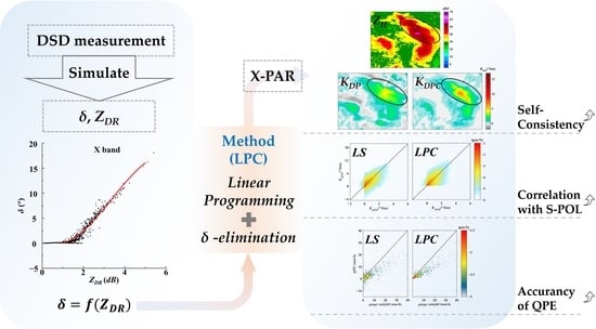
2.1. Simulation and Correction Methods Based on DSD Data

For a single hydrometeor, the backscattering matrix of the radar wave can be expressed as:
E H r E V r = e j k r r S H H S H V S V H S V V E H i E V i
where E H i and E V i are the incident electric field intensities of the horizontally and vertically polarized waves, respectively; E H r and E V r are the electric field intensities of the particle scattering; SHH, SHV, SVH, and SVV are the four complex scattering functions of the scattering matrix. The forward and backward scattering is denoted by 0° and 180°, respectively, while the DSD is denoted by N(D). Then, the δ of a single hydrometeor can be expressed as:
δ D = a r g S H H * 180 S V V 180
where * denotes the conjugate of the complex number. For a rain area with a DSD of N(D), the δ, ZV, ZH, ZDR, KDP, and specific attenuation A can be calculated by [27]
δ = arg 0 D m a x N D S H H 180 , D   S V V 180 , D e j δ D d D
Z H , V = λ 4 π 5 U 2 0 D m a x 4 π S H H , V V 180 , D 2 N D d D
Z D R = 10.0 l o g 10 Z H Z V
K D P = 180 λ π 0 D m a x R e S H H 0 , D S V V 0 , D N D d D
A H , V = 0.4343 4 π k 0 D m a x I m S H H , V V 0 , D N D d D
where U = ε 1 ε + 2 , and ε is the complex relative dielectric constant,   k = 2 π λ .
In this way, the total measured differential phase ΦDP and KDPR calculated by ΦDP can be expressed by Equations (8) and (9), respectively:
Φ D P r = δ r + 2.0 0 r K D P s d s
K D P R = K D P + δ 2 δ 1 2 r 2 r 1
The definition of δ shows that it is related to the raindrops’ size, rather than their numerical density, similar to ZDR. The effect of δ on KDP is only related to its variation with distance.
The backscattering cross-section of raindrops was calculated using the extended boundary condition method [28]. The quality-controlled data from an OTT Particle Size Velocity (PARSIVEL) disdrometer [29] at the Longmen Observatory in Guangdong Province in 2020 were used to calculate ZH, ZDR, KDP, and δ and to fit their relationships. For the 1 min resolution DSD data, the data with precipitation intensity less than 0.5 mm/h and fewer than 50 total raindrops were first removed [30], followed by the removal of data that deviated from the terminal velocity of the falling raindrops [31].
To simulate the effect of δ on the radar polarimetric variables and attenuation correction, we assumed that the precipitation system was a rigid body in uniform motion and that the precipitation parameters were homogeneous within the radar observation volume; in this way, the variation in the DSD over time could be transformed into spatial variation, and the polarimetric variables along a propagation path of the radar observations could be simulated and used to analyze the effects of δ on the KDP and correction effect.
It is known that δ and ZDR depend on the particles size and are independent of the absolute particle number density; thus, the following method for δ correction using quality-controlled ZDR was proposed:
  • Firstly, based on the local DSD data, the fitted relationship between δ and ZDR was calculated.
  • Based on this relationship, the threshold of ZDR for δ correction was determined; i.e., δ was only calculated when ZDR was larger than this threshold.
  • The elimination of δ from the filtered ΦDP was carried out:
Φ D P C = Φ D P R δ Z D R
where Φ D P R and Φ D P C represent the differential propagation phase before and after the δ elimination, respectively, and δ(ZDR) is the δ calculated using ZDR.

2.2. The X-PAR Data

The X-PAR data used in this paper were taken from the Qiuyutan station in Shenzhen, Guangdong (22.65°N, 113.85°E). This radar network was completed by the end of 2019. The X-PAR was X-band fully coherent pulsed doppler dual-polarization phased-array radar. Its peak power is 256 W, and it provides a range resolution of 30 m, 12 elevation angles, and a temporal resolution of 92 s; its 3D scan data contain polarimetric variables such as reflectivity ZH (unit: dB), correlation coefficient ρhv, differential reflectivity ZDR (unit: dB), differential propagation phase ΦDP (unit: °), and specific differential propagation phase KDP (unit: °/km). The radar data from March to September 2020 (a total of 17,863 volume scans) were processed with attenuation correction (including ZH and ZDR) based on the quasi-linear relation between path integral attenuation (PIA) and ΔΦDP (PIA = γΔΦDP). Usually, S-band dual-polarization Doppler weather radar (S-POL) undergoes rigorous calibration during the upgrade process to increase the data reliability, and the S-band signal is weakly affected by attenuation when the electromagnetic wave passes through the rain. Because of the high reliability and the same location as the X-PAR, S-POL data were used to verify the accuracy of X-PAR data. The key parameters of the two radars are listed in Table 1.

2.3. KDP Calculation Methods

The ΦDP and ZDR based on the DSD simulation data do not take other noise information from the actual radar observations into account. However, there is a large amount of random noise in the actual radar-observed ΦDP, in addition to the effect of δ, and the noise information from the ZDR is also brought into ΦDP due to δ correction. Therefore, in the process of calculating the KDP, δ correction and further denoising are required. Since filtering and denoising can also suppress the effects of δ, two filtering and denoising schemes were used to preprocess ΦDP and then calculate the KDP in order to analyze the effect of δ correction.

2.3.1. KDP Calculation Based on Low-Pass Filtering and Least Squares (LS)

KDP can be calculated directly from filtered ΦDP via the least-squares method, which is common and efficient. In this study, a 3 km moving average was used to denoise the ΦDP. This method set a low-pass filter with filter coefficients equal to the reciprocal of the span. Least-squares linear regression was then fitted to ΦDP within a total of 1 km window of each gate of the ray path, using the slope obtained from the fit to calculate the KDP for that gate.

2.3.2. KDP Calculation Based on SG Smoothing Filters and LP Method

The LP method proposed by [19] with good performance was chosen to calculate ΦDP, and the KDP consistent with the physical characteristics of the precipitation system could be obtained. The objective of LP is to minimize the difference between reconstructed φ D P f i t and observed ΦDP within the constraint that the KDP corresponding to φ D P f i t is within the interval between KDPmin and KDPmax. This objective was achieved by an LP scheme designed as follows:
Minimize c· xc
Subject to AAUG xcbAUG
x c z , x T 0
of which
  A AUG = I n I n I n I n Z n m + 1 , n M n m + 1 , n Z n m + 1 , n M n m + 1 , n
where In is the n × n identity matrix, while Zn−m+1,n is an (n − m + 1) × n matrix of zeros. The range resolution of the X-PAR is 30 m, m = 33 (i.e., 1 km), and n is the length of ΦDP.
M n m + 1 , n = d 1   d 2   d m   0 1   0 n m   0 1     0 n m   d 1   d 2   d m
d i = 6 2 i m 1 m m + 1 m 1
b AUG = Φ D P Φ D P 2 s K D P m i n 2 s K D P m a x
where Φ D P is the observational radial Φ D P data array, s is the range resolution of X-PAR, while KDPmin and KDPmax are set as the weak physical constraints for φ D P f i t , and they are 1/4 and 4 times the KDPZ calculated from ZH after attenuation correction by using the fitting formula based on DSD, respectively. Since the KDP is calculated from ΦDP by a 33-point Savitzky–Golay (SG) derivative filter, the physical constraint here is weak, which is only to avoid some extremely unreasonable ΦDP jitter.
c = t 1   t 2   t n   0 1   0 2   0 n  
t i =     1   , Q C i = 1     0.3   ,   Q C i = 0
The weight integral of z represents the difference between Φ D P and φ D P f i t ; Φ D P should be continuous within the precipitation zone, but due to observation or signal processing error, Φ D P occasionally has missing measurements or abnormal jitter at some gates. For this area of poor-quality Φ D P , linear interpolation was used to supplement it. Since these data were interpolated, a smaller weight was set in the cost function, where ti is the weight factor of z.
Finally, an LP scheme is solved to obtain xc as a 2n × 1 column matrix, where rows 1 to n are z and rows (n + 1) to 2n are x. The vector x satisfies the constraints of the LP scheme for φ D P f i t , but there are still some high-frequency fluctuations, and the vector x can be filtered by the SG smoothing filter corresponding to the SG derivative filter to obtain a smooth φ D P f i t . KDP can be calculated from φ D P f i t using the SG derivative filter.
s i = d 1 2     ,   i = 1     d i 2 1 i 1 d j   , i 2 , m + 1 2         s m i + 1   ,   i m + 1 2 + 1 , m  
N n m + 1 , n = s 1   s 2   s m   0 1   0 n m   0 1     0 n m   s 1   s 2   s m
φ D P f i t = N x                                                          

2.3.3. KDP Calculation Schemes for X-PAR

In order to test the effect of the δ-correction method, four sets of KDP calculation schemes of X-PAR were designed based on the two different KDP calculation methods mentioned above:
Exp1: A low-pass filter is applied to ΦDP to remove some of the random noise, and then the least-squares method is used to calculate KDP1.
Exp2: Based on the δ–ZDR statistical relationship, δ is calculated using the attenuation-corrected ZDR. After subtracting δ from the observed ΦDP to obtain ΦDP2, KDP2 is calculated using the method of Exp1.
Exp3: Based on the DSD measurement and fitting calculation, an equation between KDP and ZH is obtained, and then the KDPZ based on the radar-observed ZH (after attenuation correction) is calculated. The KDPZ is used as a weak physical constraint, and the LP method is used to calculate the processed ΦDP3, as well as to calculate the KDP3 [19].
Exp4: Based on the δ–ZDR statistical relationship, δ is calculated using the attenuation-corrected ZDR. After subtracting δ from the observed ΦDP to obtain ΦDP2, ΦDP4, and KDP4 are calculated using the method of Exp3.

3. Results

3.1. The Relationship of δ with Raindrops’ Size and Temperature

Firstly, the analysis shows the relationship between δ and the equivalent diameter of the raindrops at different temperatures in S-, C-, and X-bands (Figure 1). For S-, C-, and X-bands, an obvious change in the δ exists only when the equivalent diameter D of the raindrops is greater than 6 mm, 4 mm, and 2 mm, respectively. The conditions for generating δ in precipitation are easily satisfied for X-band. It is noted that δ shows a nonmonotonic change with diameter causing resonance effects at higher temperatures at C-band. In addition, there is a range of diameters that δ varies most strongly with D for each band (near 6 mm for C-band and near 4 mm for X-band). Since the effect of δ on KDP is mainly based on the variation in δ with distance, a change in the DSD in these ranges may produce a significant change in ΦDP and affect the calculation of KDP. The variation trend of δ with D is in accordance with the previous studies [7], but the amplitude of δ calculated in this paper is about 1/4 higher, which may be related to different assumptions of the raindrops shape.
The scatterplot of the distribution of δ with ZDR was calculated using DSD measurement from the Longmen observatory in Guangdong in May–June 2019 (Figure 2). Only the C- and X-band cases are given in Figure 2, considering that δ has little effect on the ΦDP and KDP of the S-band radar. The time resolution of DSD measurement is 1 min, the sample size of valid data is 85,265, with 10,001 samples with simulated reflectivity greater than 10 dBZ. According to Figure 2, δ is very small at ZDR < 1.0 dB. For this reason, we suggest that this case (ZDR < 1.0 dB) should not be processed with δ elimination for ΦDP. For X-band, the number of points with simulated ZDR > 1.0 dB is 3358, while the number of points with δ > 1.0° is 1239. In contrast, for C-band, there are 572 points with ZDR > 1.0 dB and 72 points with δ > 1.0°.
In order to compare the differences between the DSD measurement and the simulations in other articles [24], we used the gamma model, where the simulations of C- and X-band radar are given in Figure 2c,d, respectively. The gamma distribution equation is:
N D = N w D m e x p 3.67 D D 0
The m values were in the range from −1 to 4, while D0 took values in the range from 0.5 to 2.5 mm. Noted that δ has no relation with NW.
Comparing the two DSD sources, they have a consistent trend for ZDR > 2.0 dB, and the C-band results from the DSD measurement are more dispersed than the gamma model’s DSD values. The DSD measurement often deviates from the gamma parameter distribution, leading to weak correlation between the X-band δ and ZDR for ZDR < 2.0 dB. Considering the uncertainty of the parameters in the gamma distribution hypothesis, the simulation based on the DSD measurement is more accurate to the statistics of the polarimetric variables in the research area. Compare with previous studies, the fitting relationship between δ and ZDR at X-band is basically consistent with the fitting curve of [12] and δ = ZDR1.8 proposed by [25].
According to the above results, the fitting equations for X- and C-band ZDR and δ were obtained:
X-band:
δ = 0.962 3.16 Z D R + 2.44 Z D R 2 0.241 Z D R 3
C-band:
δ = 0.536 1.170 Z D R + 0.499 Z D R 2 + 0.0334 Z D R 3
To analyze the effects of δ on QPE and attenuation correction, the X-band radar QPE equations and attenuation correction equations were obtained through fitting.
R = 0.023 Z H 0.694
R = s i g n K D P 12.7 K D P 0.85
A H = s i g n K D P 0.16 K D P 0.96  
A D R = s i g n K D P 0.0247 K D P 1.18
Notably, it may seem unreasonable to calculate negative attenuation and rain intensity when the KDP is negative in Equations (24) and (25), but, in fact, this approach is justified because negative KDP is often caused by a variety of factors, especially the effects of δ and radar sampling errors, but such errors are local or random. While the negative values of KDP may match some overestimated positive KDP, when such negative rain intensity or attenuation is calculated by distance-averaging or time-averaging, these unreasonable values will be smoothed out by the accumulation to give a relatively reasonable average.

3.2. The δ-Correction Effect Based on Simulated Data

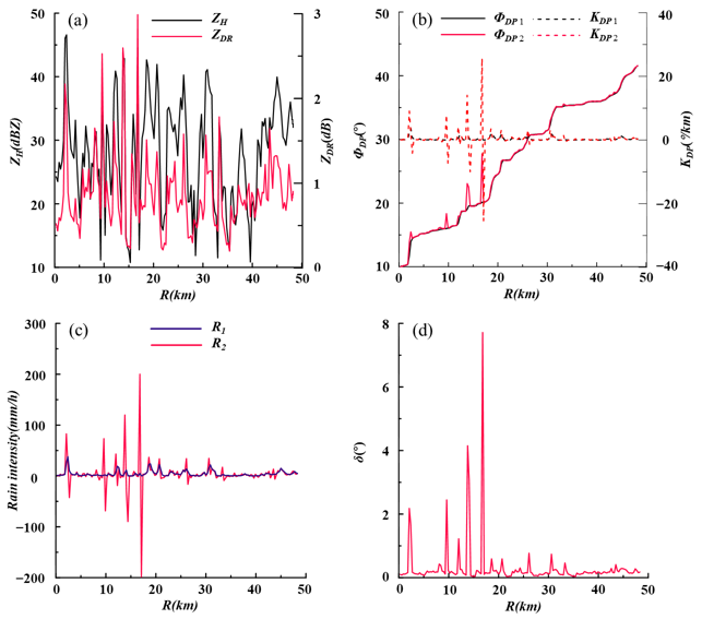
3.2.1. Simulating the Effects of δ on ФDP and KDP

Using the disdrometer DSD measurements from 12:12 to 15:58 on 10 June 2019, the polarimetric variables of an X-band radar were simulated for a 40 km radar’s radial data, with the assumption that the movement speed is 18 km/h. Figure 3 shows the variation in ZH, ZDR, ФDP1, and KDP1 (without the effect of δ), as well as that of ФDP2 and KDP2 (affected by δ, which represents actually the result of the actual radar observation), with distance for these simulated radial data. Among these radial data, ZH varies from 10 to 50 dBZ, with a ZDR range of 0–3.0 dB. It can be seen that with sudden changes in ZDR, δ can cause local variations of ±8.0° in ФDP and ±25.0°/km in KDP, far exceeding the reasonable range, overestimating KDP in areas of sudden ZDR increase and underestimating KDP in areas of ZDR decrease, sometimes even resulting in significantly negative KDP. The local mutation of ΦDP and KDP produced by δ is not negligible. For the effect of δ on QPE (Figure 3c), without the δ elimination, QPE is significantly locally underestimated and overestimated. Although the effect of δ on cumulative precipitation estimates can be mostly offset by space–time integration, its effect on rainfall intensity estimates is very severe.

3.2.2. The Effects of δ on Attenuation Correction

Under the assumption that the precipitation system is moving at a constant speed, the variation in ZH, ZDR, AH, ADR, and δ with distance of a ray path can be obtained using the time series of these polarimetric variables calculated from the DSD measurement. Using the calculated AH and ADR, the ZH and ZDR after attenuation can be obtained—that is, the simulated radar measurements’ ZH and ZDR. Additionally, based on Equations (25) and (26), the KDP can be used to calculate the AH and ADR for correction, and we can obtain the ZH and ZDR after attenuation correction and further compare them with the ZH and ZDR calculated from the DSD data to analyze the correction effect.
Figure 4 shows the ZH, ZDR, and PIA (calculated directly from the DSD and calculated from KDP affected by δ). The difference between the PIA calculated from the two datasets is the correction error. In this case, as shown in Figure 4, the attenuation causes an underestimation of ZH and ZDR by 5.2 dB and 0.78 dB, respectively, which is sufficient to cause significant errors in precipitation estimation and hydrometeor classification; e.g., ZDR may become negative after a distance of 20 km. The PIA calculated from KDP results in a smaller correction than that calculated from DSD; the magnitude of this error is distance-dependent and is mainly related to the characteristics of the DSD in the region, but the errors are all within the 1.0 dB detection error for ZH and the 0.2 dB detection error for ZDR—much smaller than the actual attenuation. Noted that the observation error of the KDP was not considered in this simulation.

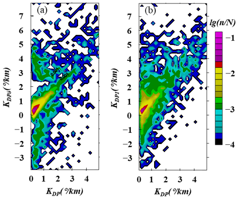
3.2.3. The Effects of δ-Elimination on KDP Calculation

In order to analyze the effect of δ elimination on the KDP calculation, the ZDR calculated from DSD without attenuation effect (Test A) and the ZDR after attenuation correction (Test B) were used to calculate the δ using Equation (11), and then the δ was eliminated from ФDPR to obtain ФDP1 (Test A) and ФDP2 (Test B), and to calculate KDP1 (Test A) and KDP2 (Test B), which were compared with the ФDP and KDP calculated by DSD simulation, respectively; finally, the rain intensity was calculated using KDP, K DP1 and KDP2 to analyze the effects of δ elimination on the rain intensity. Test A focused on the effect of the error of the δ (ZDR) fitting relation, while Test B focused on the effect of the ZDR attenuation correction error. Figure 5 shows the simulated KDP (unaffected by δ) and KDPδ (affected by δ), along with the δ-corrected KDP1 and KDP2 obtained from Test A and Test B, as well as the rain intensity calculated from these data. The calculated KDPδ (affected by δ) could be considered equivalent to the actual radar observation. As shown in Figure 5a, the local variability of KDPδ is increased due to δ, significantly, with extreme values and negative values occurring in the ZDR mutation region. Comparing Figure 5b,c reveals that the δ correction modifies the KDP error in the ZDR mutation region but also adds additional KDP local variation in the region of slow change in ZDR, which indicates the necessity of denoising after δ correction.
Based on DSD data from the Longmen Observatory in Guangdong for May–June 2019, the simulated KDP (unaffected by δ) and the simulated KDPδ (affected by δ) were calculated, along with the corrected KDP1, which was calculated based on the δ-elimination using ZDR (Figure 6b). The results show that the δ produces too many negative values of KDP as well as overestimation of KDP, especially in low-value KDP (weak rainfall) areas, and that the δ correction reduces the negative effect of δ on the KDP calculation, but there are still some errors.

3.3. The Effect of δ Correction on X-PAR KDP Calculation

3.3.1. Case Analysis on Radial Data

Taking the results of the radial data processed at 10:32 a.m. on 13 September 2020—with an elevation angle of 4.5° and an azimuth angle of 293.4°—as an example (see Figure 7), there are obvious high values of ZH and ZDR, as well as the strong fluctuations of the corresponding ΦDP, with an obvious δ characteristic near 26 km of the ray path. The δ calculated from ZDR reaches a maximum of 7.2°. The δ-eliminated ΦDP shows a relatively significant decrease in the range of 24–27 km. The ΦDP3 calculated by LP is shown in Figure 7b. Due to the physical constraints that ensure a monotonically non-negative trend of ΦDP3 with distance in the liquid precipitation, the δ- eliminated ΦDP4 differs from ΦDP3 mainly in the weak fluctuations at 24 km and the backward shift of the steeply rising section (corresponding to the region of large KDP values). KDP and ZH are mainly related to the scale and number of large oblate spherical raindrops, while the target of observation is liquid precipitation. The trends of KDP calculated by LS and LP are essentially the same, with both peaking around 25 km, but the δ-corrected KDP is more consistent with the trend of ZH. This is because δ increases ΦDP in the large raindrops zone and, thus, causes an overestimation of KDP at the front of the large raindrops zone, while δ decreases after the large raindrops zone, which also causes an underestimation of KDP at the back of the large raindrops zone. After the δ correction, the KDP values calculated by both LS and LP were more consistent with the ZH trend. On the other hand, despite the filtering process, the KDP calculated by LS still had some negative values in the liquid precipitation, which was inconsistent with the non-negative KDP corresponding to the oblate spherical characteristics of raindrops, while the KDP calculated by LP—due to the physical constraints—ensured the non-negative characteristics.

3.3.2. Case Analysis on PPI

Taking a strong convective weather process as an example, in the northeast direction of the X-PAR at 01:20 on 8 June 2020. To analyze the performance of KDP estimation to fine structures, we selected a small research area with only 15 km. Thanks to the high spatial resolution, X-PAR has observed a hook echo structure of the convective cell, while S-POL was difficult to show such detailed characteristics.
Because there is a time difference (≤1 min) between the two radars’ measurements, and the position of the same echo is slightly mismatched, the relative position of each polarimetric variable was the main focus of the analysis. In terms of S-POL observation, the high-value positions of ZH, ZDR, and KDP of A and B cells were basically consistent; although, the detailed characteristics of KDP were insufficient due to the low resolution.
For Exp1 (Figure 8f) and Exp3 (Figure 8h) without δ correction, the high value centers of KDP of cell A are shifted southward relative to the ZH high value, which was improved with δ correction of Exp2 (Figure 8g) and Exp4 (Figure 8i), and the KDP of cell B with δ non-corrected has a similar situation. This problem is manifested in the relative expansion of the high-value range, the underestimation of high value, and the poor self-consistence with ZH and ZDR. After δ correction, the maximum value of KDP of cell B was more reasonable (consistent with S-POL), and the structure of KDP was also more consistent with ZH and ZDR. In addition, the false increase in ΦDP caused by δ will also result in an unreasonable negative value (Figure 8f) behind the KDP peak by the LS method. Through δ correction, the negative values of KDP at the back side (north side) of cell A and B were significantly improved (Figure 8g). The LP method with physical constraints solves this problem more strictly than the LS method. In a word, through smoothing filtering, Exp1 and Exp3 can obtain relatively stable KDP estimation. However, the δ, which was not completely eliminated, still affected the magnitude, position, and structure of KDP around the large particle area, which is unfavorable for the detailed analysis of cloud physical characteristics. δ correction can be helpful to solve this problem.

3.3.3. Statistical Analysis

Furthermore, the effect of δ elimination on the calculation of X-PAR KDP was tested statistically by S-POL KDP and the X-PAR attenuation-corrected ZH and ZDR. By fitting the DSD data, the statistical relation between KDP of S-band and X-band radar was obtained, and the standard value of KDP for X-PAR could be calculated from the S-POL observations via the fitting equation. In addition, there is internal self-consistency of the polarimetric variables. ZH, ZDR, and KDP are related to the scale, shape, and number of spherical raindrops, with nonlinear correlation (KDP = aZHbZDRc). Therefore, the determination coefficient of the nonlinear correlation between ZH, ZDR, and KDP can also be used to test the effect of δ correction on the accuracy of KDP estimation.
In order to reduce the errors caused by inaccurate gate-matching, only the gates with a time difference of less than 30 s between the two radar observations were selected for calculation and comparison, from which a total of 4,578,385 points with ZDR ≥ 1 dB were selected. The statistical results of four experiments are shown in Table 2. These δ-corrected KDPs obtained from both the LS and LP are more consistent with the S-POL KDP. The self-consistent analysis shows a similar result; the determination coefficient of three polarimetric variables (ZH, ZDR, and KDP) was improved after δ correction for both LS and LP—mainly due to the δ result in the overestimated KDP at the front of the large raindrops region and the underestimated KDP behind the large raindrops region. This effect was mitigated by the δ correction, and the accuracy of KDP in the large raindrops region was improved.
Figure 9 shows the calculation results of Exp2 and Exp4, mainly showing the difference between the calculation of KDPX by the LS method and LP method. Although the statistical errors of the two groups are close (as shown in Table 2), there are obvious differences in their distribution. Especially for the part of weak precipitation (low KDP value), the random noise of ΦDP may bring serious errors in the calculation of KDP, which is reflected in the weak consistency between calculated KDPX and low KDPS, as well as KDPX and low KDPM, as shown in Figure 9a,c. By contrast, the weak physical constraints of LP ensure the non-negativity of KDPX in the liquid precipitation, which is an important reason for the more accurate low KDP than using LS (as shown in Figure 9b,d).

3.3.4. QPE Test

One of the important applications of KDP is QPE; however, the noise of ΦDP makes it difficult to accurately calculate KDP in weak rainfall areas. Therefore, KDP is generally not used to calculate the precipitation intensity in the weak rainfall area [32,33]. Theoretically, the noise of ΦDP should be well suppressed via the δ correction and LP processing, and then the accurate KDP in the weak rainfall area can be obtained. In this paper, we calculated QPE based on the R-KDP relationship fitted by DSD, and then tested the accuracy of KDP of four experiments based on the local rainfall gauges (874 sets of 1 h rainfall).
In order to test the accuracy of QPE for different precipitation intensities, the errors of weak rainfall cases with precipitation intensity ≤5 mm and moderate and strong rainfall cases with precipitation intensity >5 mm are tested, respectively. On the whole, the R(KDP) calculated by LP combined with δ correction is the best (as shown in Table 3).
Affected by noise, the relative mean absolute error (RMAE = 96.4) from the LS method in weak rainfall areas is far larger than its RMAE (51.7%) in the rainfall area above 5 mm/h. In comparison, the RMAE (42.6%) of the LP method in weak rainfall areas is even slightly better than that in moderate and strong rainfall areas (48.1%). The LP method can obtain a more accurate estimation of KDP in weak rainfall areas and improve the application ability of KDP in QPE (as shown in Figure 10).
With the δ correction, the accuracy of KDP estimation was improved, and the error of QPE was reduced. The improvement in KDP accuracy in weak rainfall areas was better than that in strong rainfall areas. However, for the LS method, in the part of the rainfall > 5 mm/h, Exp2 is slightly higher than Exp1 in RMAE. The reason is that strong rainfall is often accompanied by a large δ estimation, and the errors of ZDR and calculation errors of δ would be brought into the estimation of KDP. The LP method with physical constraints can better suppress these errors.

4. Discussion

The δ observed by S-, C-, and X-band weather radar at different temperatures for various raindrop sizes was simulated using the OTT PARSIVEL laser disdrometer. For comparison, in the liquid precipitation region, S-band radar was less affected by δ, and the δ in C- and X-bands varied sharply with raindrop sizes of 6 mm and 4 mm. Due to the influence of δ on KDP calculation—mainly as a result of the variation in δ with radial distance—the ΦDP of X-band weather radar observations is susceptible to δ during heavy precipitation, which further affects the KDP calculations.
Based on the analysis of the physical properties of the polarimetric variables, both δ and ZDR are highly correlated with the precipitation’s particle size, while they are insensitive to the particle number concentration. It is feasible to calculate and fit ZDR and δ using DSD data. For X-band weather radar, the value of δ is small (about zero) at ZDR < 1 dB, and there is a positive correlation between ZDR and δ at ZDR > 1 dB. The fitting result is basically consistent with δ = ZDR1.8 proposed by [25].
By simulating the radar-sounding data from disdrometer DSD measurements, it was found that for ZDR within a 3 dB variation, there was local variation with a maximum of ±8° to ΦDP and ±25.0°/km to KDP. While this effect can be suppressed in cumulative precipitation, it has a large impact on local estimates of rain intensity. As the specific attenuation has a quasilinear relationship with KDP—which is often used for attenuation correction of reflectivity—the δ may cause errors in KDP, as well as having a negative effect on the attenuation correction. However, δ is not an integral variable, and its effect on the attenuation correction is local. Based on the polarimetric variables simulated from DSD, the effect of δ on the attenuation correction is not very significant in the holistic radial observation. The estimation of KDP without δ correction shows excessive fluctuations in the ZDR mutation region, which could be suppressed by fitting the ZDRδ relationship and δ elimination.
KDP was calculated based on different calculation schemes using the observations of X-PAR deployed in Shenzhen, China. The ФDP preprocessing is generally achieved via filtering or reconstruction. Even if the expected value of KDP is used as a physical constraint, the LP method for ΦDP preprocessing can only be used as a weak constraint to avoid unreasonable jitter of KDP. Although these methods have inhibitory effects on the jitter of ΦDP due to δ, the influence of δ still exists, causing overestimation of ΦDP at the front of the large raindrop area of the ray path, along with further overestimation and underestimation of KDP in this region. With δ correction and subsequent filtering, the effects of δ could be better eliminated than with that of simple filtering. Both the estimation of KDP via LS and LP could benefit from δ correction. This optimization was verified by the improved self-consistency of polarimetric variables, the correlation between KDP calculations from S and X-band radar and the accuracy of QPE. These improvements are beneficial to the application of KDP in fine analysis of cloud physics and QPE. Notably, the δ correction may introduce errors, and the statistical results of QPE show that the LP method is better than the simple filtering method in suppressing such errors.
The positive effect of δ correction on KDP calculation was demonstrated by comparative test and analysis. Moreover, the comparison with S-POL shows that even though the beam width of X-PAR is wider, it still has a good detection performance, and the observation of X-PAR and S-POL are highly consistent, indicative of the relatively high potential for applications in radar network observations and radar mosaic.

Author Contributions

Conceptualization, L.L.; methodology, F.G. and L.L.; software, F.G. and L.L.; validation, F.G. and L.L.; formal analysis, F.G. and L.L.; investigation, F.G. and L.L.; resources, L.L.; data curation, F.G. and L.L.; writing—original draft preparation, F.G. and L.L.; writing—review and editing, F.G.; visualization, F.G. and L.L.; supervision, L.L.; project administration, L.L.; funding acquisition, L.L. All authors have read and agreed to the published version of the manuscript.

Funding

This research was funded by the National Natural Science Foundation of China (Grant No. U2142210).

Data Availability Statement

Not applicable.

Conflicts of Interest

The authors declare no conflict of interest.

Abbreviations

X-PARX-band dual-polarization phased-array weather radar
S-POLS-band dual-polarization Doppler weather radar
DSDraindrop size distribution
δbackscatter differential phase
KDPspecific differential propagation phase
Zreflectivity
ΦDPdifferential propagation phase
ZDRdifferential reflectivity factor
ρHVcorrelation coefficient
QPEquantitative precipitation estimation
PIApath integral attenuation
LPLinear Programming
LSLeast Squares

References

  1. Chandrasekar, V.; Bringi, V.N. Error structure of multiparameter radar and surface measurements of rainfall. Part iii: Specific differential phase. J. Atmos. Ocean. Technol. 1988, 5, 783–795. [Google Scholar] [CrossRef]
  2. Bringi, V.N.; Chandrasekar, V.; Hubbert, J.; Gorgucci, E.; Randeu, W.L. Raindrop size distribution in different climatic regimes from disdrometer and dual-polarized radar analysis. J. Atmos. Sci. 2003, 60, 354–365. [Google Scholar] [CrossRef]
  3. Ryzhkov, A.V.; Zrnić, D.S. Comparison of dual-polarization radar estimators of rain. J. Atmos. Ocean. Technol. 1995, 12, 249–256. [Google Scholar] [CrossRef]
  4. Matrosov, S.Y.; Kropfli, R.A.; Reinking, R.F.; Martner, B.E. Prospects for measuring rainfall using propagation differential phase in x- and ka-radar bands. J. Appl. Meteorol. 1999, 38, 766–776. [Google Scholar] [CrossRef]
  5. Matrosov, S.Y.; Clark, K.A.; Martner, B.E.; Tokay, A. X-band polarimetric radar measurements of rainfall. J. Appl. Meteorol. 2002, 41, 941–952. [Google Scholar] [CrossRef]
  6. Cao, Q.; Zhang, G.; Xue, M. A variational approach for retrieving raindrop size distribution from polarimetric radar measurements in the presence of attenuation. J. Appl. Meteorol. Climatol. 2013, 52, 169–185. [Google Scholar] [CrossRef] [Green Version]
  7. Yoshikawa, E.; Chandrasekar, V.; Ushio, T.; Matsuda, T. A bayesian approach for integrated raindrop size distribution (dsd) retrieval on an x-band dual-polarization radar network. J. Atmos. Ocean. Technol. 2015, 33, 377–389. [Google Scholar] [CrossRef]
  8. Kim, D.S.; Maki, M.; Lee, D.-I. Retrieval of three-dimensional raindrop size distribution using x-band polarimetric radar data. J. Atmos. Ocean. Technol. 2010, 27, 1265–1285. [Google Scholar] [CrossRef]
  9. Besic, N.; Figueras i Ventura, J.; Grazioli, J.; Gabella, M.; Germann, U.; Berne, A. Hydrometeor classification through statistical clustering of polarimetric radar measurements: A semi-supervised approach. Atmos. Meas. Tech. 2016, 9, 4425–4445. [Google Scholar] [CrossRef] [Green Version]
  10. Gorgucci, E.; Scarchilli, G.; Chandrasekar, V. Specific differential phase estimation in the presence of nonuniform rainfall medium along the path. J. Atmos. Ocean. Technol. 1998, 16, 1690–1697. [Google Scholar] [CrossRef]
  11. Gosset, M. Effect of nonuniform beam filling on the propagation of radar signals at x-band frequencies. Part ii: Examination of differential phase shift. J. Atmos. Ocean. Technol. 2004, 21, 358–367. [Google Scholar] [CrossRef]
  12. Testud, J.; Bouar, E.L.; OBligis, E.; Ali-Mehenni, M. The rain profiling algorithm applied to polarimetric weather radar. J. Atmos. Ocean. Technol. 2000, 17, 332–356. [Google Scholar] [CrossRef]
  13. Trömel, S.; Kumjian, M.R.; Ryzhkov, A.V.; Simmer, C.; Diederich, M. Backscatter differential phase—Estimation and variability. J. Appl. Meteorol. Climatol. 2013, 52, 2529–2548. [Google Scholar] [CrossRef] [Green Version]
  14. Hubbert, J.; Chandrasekar, V.; Bringi, V.N.; Meischner, P. Processing and interpretation of coherent dual-polarized radar measurements. J. Atmos. Ocean. Technol. 1993, 10, 155–164. [Google Scholar] [CrossRef]
  15. Hubbert, J.; Bringi, V.N. An iterative filtering technique for the analysis of copolar differential phase and dual-frequency radar measurements. J. Atmos. Ocean. Technol. 1995, 12, 643–648. [Google Scholar] [CrossRef]
  16. Schneebeli, M.; Berne, A. An extended kalman filter framework for polarimetric x-band weather radar data processing. J. Atmos. Ocean. Technol. 2010, 29, 711–730. [Google Scholar] [CrossRef]
  17. Wen, G.; Fox, N.; Market, P. A gaussian mixture method for specific differential phase retrieval at x-band frequency. Atmos. Meas. Tech. 2019, 12, 5613–5637. [Google Scholar] [CrossRef] [Green Version]
  18. Reinoso-Rondinel, R.; Unal, C.; Russchenberg, H. Adaptive and high-resolution estimation of specific differential phase for polarimetric x-band weather radars. J. Atmos. Ocean. Technol. 2018, 35, 555–573. [Google Scholar] [CrossRef]
  19. Giangrande, S.E.; Mcgraw, R.; Lei, L. An application of linear programming to polarimetric radar differential phase processing. J. Atmos. Ocean. Technol. 2013, 30, 1716–1729. [Google Scholar] [CrossRef]
  20. Huang, H.; Zhang, G.; Zhao, K.; Giangrande, S. A hybrid method to estimate specific differential phase and rainfall with linear programming and physics constraints. IEEE Trans. Geosci. Remote Sens. 2017, 55, 96–111. [Google Scholar] [CrossRef]
  21. Ma, J.; Chen, M.; Li, S.; Yang, M. Application of linear programming on quality control of differential propagation phase shift data for x-band dual linear polarimetric doppler weather radar. Acta Meteorol. Sin. 2019, 77, 516–528. [Google Scholar] [CrossRef]
  22. Reimel, K.; Kumjian, M. Evaluation of kdp estimation algorithm performance in rain using a known-truth framework. J. Atmos. Ocean. Technol. 2020, 38, 587–605. [Google Scholar] [CrossRef]
  23. Helmus, J.; Collis, S. The python arm radar toolkit (py-art), a library for working with weather radar data in the python programming language. J. Open Res. Softw. 2016, 4, 25. [Google Scholar] [CrossRef] [Green Version]
  24. Scarchilli, G.; Goroucci, E.; Chandrasekar, V.; Seliga, T.A. Rainfall estimation using polarimetric techniques at c-band frequencies. J. Appl. Meteorol. 1993, 32, 1150–1160. [Google Scholar] [CrossRef]
  25. Otto, T.; Russchenberg, H.W.J. Estimation of specific differential phase and differential backscatter phase from polarimetric weather radar measurements of rain. Geosci. Remote Sens. Lett. IEEE 2011, 8, 988–992. [Google Scholar] [CrossRef]
  26. Zhang, W.; Wu, C.; Liu, L.; Zhang, Y.; Bao, X.; Huang, H. Research on Quantitative Comparison and Observation Precision of Dual Polarization Phased Array Radar and Operational Radar. Plateau Meteorol. 2021, 40, 424–435. [Google Scholar] [CrossRef]
  27. Bringi, V.N.; Chandrasekar, V. Polarimetric Doppler Weather Radar: Principles and Applications; Cambridge University Press: Cambridge, UK, 2001; ISBN 9780521623841. [Google Scholar]
  28. Barber, P.; Yeh, C. Scattering of electromagnetic waves by arbitrarily shaped dielectric bodies. Appl. Opt. 1975, 14, 2864–2872. [Google Scholar] [CrossRef]
  29. Wu, Y.; Liu, L. Statistical characteristics of raindrop size distribution in the Tibetan Plateau and southern China. Adv. Atmos. Sci. 2017, 34, 727–736. [Google Scholar] [CrossRef]
  30. Tokay, A.; Petersen, W.A.; Gatlin, P.; Wingo, M. Comparison of raindrop size distribution measurements by collocated disdrometers. J. Atmos. Ocean. Technol. 2013, 30, 1672–1690. [Google Scholar] [CrossRef]
  31. Jaffrain, J.; Berne, A. Experimental quantification of the sampling uncertainty associated with measurements from parsivel disdrometers. J. Hydrometeorol. 2011, 12, 352–370. [Google Scholar] [CrossRef]
  32. Chen, H.; Chandrasekar, V. The quantitative precipitation estimation system for dallas-fort worth (dfw) urban remote sensing network. J. Hydrol. 2015, 531, 259–271. [Google Scholar] [CrossRef] [Green Version]
  33. Diederich, M.; Ryzhkov, A.; Simmer, C.; Zhang, P.; Troemel, S. Use of specific attenuation for rainfall measurement at x-band radar wavelengths. Part II: Rainfall Estimates and Comparison with Rain Gauges. J. Hydrometeorol. 2015, 16, 503–516. [Google Scholar] [CrossRef]
Figure 1. The relationship between δ and raindrops’ equivalent diameter for (a) S-, (b) C-, and (c) X-band at different temperatures.
Remotesensing 15 01334 g001
Figure 2. Scatterplots of the δ calculated from DSD measurement with ZDR for the (a) C-band and (b) X- band, and of δ calculated from gamma assumptions of DSD with ZDR for the (c) C-band and (d) X- band. The red line represents the polynomial-fitted δ–ZDR relationship curve.
Remotesensing 15 01334 g002
Figure 3. Simulated (a) ZH and ZDR curves with distance using DSD measurements from 12:12 to 15:58 on 10 June 2019, (b) ΦDP and KDP calculated from DSD with δ effects (red curve) and without δ effects (black curve), (c) Rain intensity calculated by KDP without δ effects (R1, blue curve) and with δ effects (R2, red curve), and (d) Backscatter differential phase.
Remotesensing 15 01334 g003
Figure 4. Comparison of the actual attenuation and attenuation correction for (a) ZH and (b) ZDR. The black line shows ZH or ZDR, the red solid line shows the actual PIA for reflectivity and path integrated differential attenuation (PIDA) for differential reflectivity, and the blue line shows the attenuation correction (PIAδ and PIDAδ); the differences between the red and blue curves are the errors in the attenuation correction caused by δ.
Remotesensing 15 01334 g004
Figure 5. (a) KDP (unaffected by δ) and KDPδ calculated from ΦDPR (affected by δ); (b) KDP1 after the elimination of δ from ΦDPR using the ZDR without attenuation effect, and KDP2 using the corrected ZDR, KDP1, and KDP2 denote the corrected KDP for the two tests, respectively; (c) rain intensity estimated from KDP1 (R1) and KDP2 (R2); (d) the actual rainfall intensity.
Remotesensing 15 01334 g005
Figure 6. Colored density plot of the simulated KDP versus (a) the KDPδ affected by δ and (b) the corrected KDP1 based on the δ-elimination using ZDR.
Remotesensing 15 01334 g006
Figure 7. Typical radar sounding of (a) ΦDP, ZDR, and δ obtained by ZDR, and ΦDP2 obtained by δ correction; (b) LP-processed results obtained before (blue curve) and after (red curve) δ correction; (c) ZH after attenuation correction (dBZ) and KDP before and after δ correction using LS; and (d) ZH after attenuation correction (dBZ) and KDP before and after δ correction using LP.
Remotesensing 15 01334 g007
Figure 8. Radar PPI of (a) ZH from S-POL, (b) ZDR from S-POL, (c) KDP from S-POL, (d) ZH from X-PAR, (e) ZDR from X-PAR, (f) KDP from X-PAR calculated by Exp1 (LS without δ-elimination), (g) KDP from X-PAR calculated by Exp2 (LS with δ-elimination), (h) KDP from X-PAR calculated by Exp3 (LP without δ-elimination), (i) KDP from X-PAR calculated by Exp4 (LP with δ-elimination).
Remotesensing 15 01334 g008
Figure 9. Based on the δ-elimination processing of ΦDP, this figure shows the distribution of (a) KDPS from S-POL vs. KDPX calculated by LS, (b) KDPS from S-POL vs. KDPX calculated by LP, (c) KDPM calculated using fitting relation of polarimetric variables vs. KDPX calculated by LS, (d) KDPM calculated using fitting relation of polarimetric variables vs. KDPX calculated by LP.
Remotesensing 15 01334 g009
Figure 10. Colored density plot of 1 h rainfall by rain gauges vs. (a) QPE by EXP1 KDP (LS without δ-elimination) and (b) QPE by EXP4 KDP (LP with δ-elimination).
Remotesensing 15 01334 g010
Table 1. X-PAR and S-POL radar parameters.
Radar ParametersX-PARShenzhen S-POL
Frequency9.3~9.5 GHz2.8 GHz
Peak power256 W≥650 kW
Update time92 s360 s
Range coverage42 km230 km
Range resolution30 m250 m
Elevation scan range0.9°~20.7° with 1.8° step0.5~19.5°, 9 layers
BeamwidthsHorizontal: 3.6°; vertical: 1.8°Horizontal: <1°; vertical: <1°
Array plane normal angle15°/
Scan modeVolume range height indicator scanVolume plan position indicator scan
Table 2. Accuracy and error statistics of KDP obtained from four tests.
S-POL TestSelf-Consistency Test
TestMAERMSECCR2RMSE
Exp10.741.140.730.600.96
Exp20.711.110.750.640.94
Exp30.731.160.730.620.95
Exp40.711.130.750.660.92
Table 3. Error statistics of QPE by R (KDP).
TestMAE (mm/h)RMSE (mm/h)RMAE (%)CC
All casesExp14.517.0259.180.78
Exp24.516.9859.190.79
Exp33.616.3247.370.89
Exp43.606.2747.190.89
Rainfall ≤5 mm/hExp12.203.3596.440.31
Exp22.193.3396.220.32
Exp30.981.3343.120.58
Exp40.971.3142.570.59
Rainfall >5 mm/hExp17.509.9251.650.77
Exp27.519.8651.700.78
Exp37.009.4448.230.82
Exp46.999.3748.120.83
Disclaimer/Publisher’s Note: The statements, opinions and data contained in all publications are solely those of the individual author(s) and contributor(s) and not of MDPI and/or the editor(s). MDPI and/or the editor(s) disclaim responsibility for any injury to people or property resulting from any ideas, methods, instructions or products referred to in the content.

