Article

Study on Attenuation Correction for the Reflectivity of X-Band Dual-Polarization Phased-Array Weather Radar Based on a Network with S-Band Weather Radar

1
School of Atmospheric Physics, Nanjing University of Information Science and Technology, Nanjing 210044, China
2
State Key Laboratory of Severe Weather, Chinese Academy of Meteorological Science, Beijing 100081, China
*
Author to whom correspondence should be addressed.
Remote Sens. 2023, 15(5), 1333; https://doi.org/10.3390/rs15051333
Submission received: 23 January 2023 / Revised: 20 February 2023 / Accepted: 23 February 2023 / Published: 27 February 2023

Abstract

:
X-band dual-polarization phased-array weather radars (X-PARs) have been used in South China extensively. Eliminating the attenuation and system bias of X-band radar data is the key to utilizing the advantage of X-PAR networks. In this paper, the disdrometer raindrop-size distribution (DSD) measurements are used to calculate the radar polarimetric variables and analyze the characteristics of precipitation attenuation. Furthermore, based on the network of S-band dual-polarization Doppler weather radar (S-POL) and X-PARs, an attenuation-correction method for X-PAR reflectivity is proposed with S-POL constraints in view of the radar-mosaic requirements of a multi-radar network. Linear programming is used to calculate the attenuation-correction parameters of different rainfall areas, which realizes the attenuation correction for X-PAR. The results show that the attenuation-correction parameters simulated based on the disdrometer DSD vary with different precipitation classification; the attenuation-corrected reflectivity of X-PARs is consistent with S-POL and can realize a more precise observation of the evolution of the convective system. Compared with previous attenuation-correction methods with constant correction parameters, the improved method can reduce the deviation between X-PAR reflectivity and that of S-POL in heavy rainfall areas and areas of strong attenuation. The method proposed in this paper is stable and effective. After effective quality control, it is found that the X-PAR network deployed in South China observes data accurately and is consistent with S-POL; thus, it is expected to achieve high temporal–spatial resolution within a radar mosaic.

1. Introduction

Restricted by factors such as Earth’s curvature, electromagnetic-wave refraction, geography, and scan mode, there is a fade zone in the observation of remote low-layer weather processes that lowers the ability to monitor and warn for hazardous weather in low-altitude areas, especially in areas with complex geography or sparse radar-station networks. An X-band weather-radar network can greatly enrich the observation of the S-band-based operational radar network. It can especially enrich the low-layer observation with high temporal–spatial resolution, which is of great significance to the observation, assimilation, short-term forecast, and precipitation estimation of strong convective weather. In terms of the latest development trends of international meteorological radars, in order to improve monitoring and early warning capabilities regarding strong convective weather, X-PAR networks have recently been applied in meteorological service and research in many regions of China [1,2]. However, X-band radars with short wavelengths were seriously affected by attenuation in heavy rainfall areas compared with S-band radars. Therefore, strict quality control must be carried out. In addition, a multi-radar network mosaic is necessary to obtain large-scale precipitation data and solve the limitations of the small-range detection of X-PAR. The accurate quality control of X-PAR to ensure consistency between X-PAR and S-POL radar is the key to a networked radar mosaic.
For dual-polarization radar, the ZPHI method (rain-profiling algorithm), based on the exponential relationship between specific attenuation (AH) and reflectivity (ZH) and the quasi-linear relationship (the coefficient is denoted as γ) between AH and specific differential propagation phase (KDP) [3,4], is an important method for attenuation correction. γ is a key parameter in the ZPHI algorithm. There have been many studies on the estimation of γ based on simulated DSD data. For X-band radar, the value of γ is generally in the range of 0.2–0.3 dB/° [5,6,7,8]. However, since γ is affected by temperature, DSD, and the relationship of drop shape versus size, a constant γ may bring errors in correction. Therefore, some self-consistent methods were proposed by [9,10,11,12,13] to obtain the optimal γ solution based on the internal self-consistency of the polarimetric variables [14]. Self-consistent methods take into account the difference in raindrop characteristics and can obtain fine γ estimation, but there may be no solution in weak attenuation areas.
Similarly, radar-networked observation provides another consistency that can be used for attenuation correction; that is, the physical quantities observed by multiple radars at the same atmospheric volume should be consistent after reasonable conversion. For an X-band weather-radar network, the γ and intrinsic reflectivity could be calculated under the assumption that the differences in networked radars in the same atmospheric volume were due to attenuation only. Factors such as range-resolution volume and pointing mismatch for common volume, signal fluctuation, and bias errors that can introduce errors were evaluated using synthetic X-band observations, and the results showed that the accuracy of correction was not much affected by those factors [15,16]. Since long-wavelength (C- or S-band) radar is less affected by attenuation, path-integrated attenuation (PIA) could be calculated by the difference between the reflectivity of long-wavelength radar and X-band radar and further used for attenuation correction [17,18,19]. However, these methods ignore the possible differences of attenuation correction parameters in large-scale precipitation.
The constraint condition of the attenuation-correction method based on radar-networked observation is that multi-radars have consistent observation data in the same atmospheric volume. One of the main applications of X-PAR is to obtain a more accurate precipitation-radar observation by improving the temporal resolution and low-layer detection capabilities with a network radar mosaic with an S-POL radar network. The key to this method lies in eliminating the attenuation effect and system bias of X-band radar to achieve overall consistency of S- and X-band radar data. Taking the X-PAR and S-POL network as an example, in Shenzhen, South China, an efficient and accurate attenuation-correction method for X-PAR reflectivity is explored in this study. The DSD data are used to simulate radar-polarimetric variables and calculate the conversion relationship of different bands of radar observations as well as the relevant parameters of attenuation correction. Furthermore, an attenuation-correction method is proposed based on the advantages of radar networks with precipitation classification and correction parameters calculated via linear programming. It is hoped that efficient and accurate attenuation correction can be achieved to ensure overall consistency between the X-PARs and S-POL so as to facilitate the observation of regional-precipitation weather systems and the multi-radar network mosaic in the future.

2. Data and Methods

2.1. Analysis Based on Disdrometer DSD Measurement

The OTT Particle Size Velocity (PARSIVEL) laser disdrometer DSD measurement [20] (at 114.1°E, 23.5°N, from April 2019 to April 2022) was used to calculated radar-polarimetric variables in this paper. This disdrometer DSD with 1 min resolution could measure the size and falling-terminal velocity of hydrometeors ranging from 0.06 mm to 24.5 mm and from 0.05 m/s to 20.8 m/s, respectively, which were divided into 32 non-equant bins. For the disdrometer DSD measurement data, precipitation intensities of less than 0.5 mm/h and with fewer than 50 total raindrops were first removed [21], followed by the removal of data that deviated from the terminal velocity of the falling raindrops [22].
We assumed that the symmetry axis of the raindrop was the vertical direction, the temperature was 10 °C, and the relation of size–shape for raindrops was set according to [23]. The scattering cross-section of raindrops was calculated via the extended boundary-condition method [24]. Using the following Equations (1)–(3), the polarimetric variables (ZH,V, KDP, AH,V) were simulated, which were further used to obtain the parameters for attenuation correction via fitting analysis.
Z H , V = λ 4 π 5 U 2 0 D m a x 4 π S H H , V V 180 , D 2 N D d D
K D P = 180 λ π 0 D m a x R e S H H 0 , D S V V 0 , D N D d D      
A H , V = 0.4343 4 π k 0 D m a x I m S H H , V V 0 , D N D d D              
where λ is the radar wavelength, D is the diameter of the raindrops, U = (ε − 1)/(ε + 2), and ε is the complex relative dielectric constant. SHH, SVV are the elements of the scattering matrix, k = 2π/λ.

2.2. Radar Data

The observation data of 27,972 scans from May to September 2020 from an S-POL and two X-PARs were used in this paper. The S-POL provided three-dimensional-volume scanning data with a range resolution of 250 m, 9 elevation angles, and a temporal resolution of 6 min, as the transmit power was 650 kW. The X-PAR was an X-band fully coherent pulsed doppler dual-polarization phased-array radar. Its peak power was 256 W, and it provided three-dimensional-volume scanning data, including reflectivity ZH (unit: dBZ), the correlation coefficient ρhv, differential reflectivity ZDR (unit: dB), differential phase ΦDP (unit: °), and specific differential phase KDP (unit: °/km) based on a range resolution of 30 m, 12 elevation angles, and a temporal resolution of 92 s. The key parameters of X-PAR and S-POL are listed in Table 1.
The S-POL was located at the Qiuyutan station, Shenzhen, Guangdong (22.65°N, 113.85°E), and the two X-PARs were located at 22.65°N, 113.85°E and 22.48°N, 114.56°E, respectively; that is, X-PAR1 was at the same site as the S-POL, and X-PAR2 was southeast of the S-POL. This radar-network was completed by the end of 2019. The locations of the three radars and the corresponding Digital Elevation Model (DEM) are shown in Figure 1.

2.3. Previous Attenuation Correction

The exponential relationship between AH and ZH in Equation (4) was proposed by [25], which can be used in the solution of AH and ZH. Note that the parameter a is variable and uncertain. In the process of the calculation of path-integrated attenuation (PIA), due to the inaccuracy of a, the error would be accumulated constantly along the ray path and be large at the end of the ray path.
A H = a Z H b
where a, b are parameters of attenuation correction; AH is specific attenuation; ZH is reflectivity (unit: mm6/m3); and H denotes a horizontally polarized wave.
With the development of dual-polarization weather-radar technology, the phase difference between horizontally and vertically polarized waves can be used to calculate the specific differential phase (KDP). The KDP is related to the size, shape, and number concentration of precipitation particles and is not affected by the electromagnetic wave-signal attenuation, and therefore is applicable to attenuation calculation. In the exponential relationship between KDP and AH in Equation (5), μ is close to 1 so that KDP has a quasi-linear relationship with AH [6].
A H = γ K D P μ
φ D P r = Φ D P r δ r = 2 0 r K D P s d s
where δ is the backscatter differential phase, and the overall measured differential phase ΦDP is a combination of the backscatter differential phase (δ) and the two-way propagation differential phase φDP [26].

2.3.1. DP Method

Based on the quasi-linear relationship assumption between KDP and AH, the PIA and the intrinsic reflectivity factor Z c could be calculated using measured reflectivity Z m , γ, and φ D P , where r is the arbitrary gate on the ray path (hereafter referred to as DP method).
P I A r = γ Δ φ D P 0 , r
10 l o g 10 Z c r = 10 l o g 10 Z m r + P I A r
To X-band radar, the Φ D P preprocessing is required to obtain φDP by suppressing δ. However, it is difficult to eliminate the influence of δ completely. According to Equation (7), the PIA of the ray path depends on the accuracy of γ and ΦDP preprocessing, which may cause error in ΦDP preprocessing to be introduced into the attenuation correction.

2.3.2. ZPHI Method

Based on Equation (4) and the constraint of Equation (7), ZPHI (rain-profiling algorithm) was proposed by [3]. This algorithm (as in Equations (9)–(12)) avoids the influence of the uncertainty of a and reduces the sensitivity of AH to the Φ D P preprocessing.
A H r = Z m b r × 10 0.1 b γ Δ φ D P 1 I r 1 , r 0 + 10 0.1 b γ Δ φ D P 1 I r , r 0   , r r 1 , r 0
Δ φ D P = φ D P r 0 φ D P r 1
I r 1 , r = 0.46 b r 1 r Z m b s d s
10 l o g 10 Z c r = 10 l o g 10 Z m r + 2 r 1 r A H s d s
where r1 and r0 are integration bounds, Zc is the corrected reflectivity (unit: mm6/m3), and Zm is the measured reflectivity (unit: mm6/m3).

2.3.3. Self-Consistent Method

In the ZPHI algorithm, b is a constant, but the value of γ is affected by the temperature, DSD, and shape-versus-size relationship of precipitation particles [27]. A self-consistent method constrained by φ D P was proposed to estimate γ [9], that is, setting a cost function to obtain optimal γ by minimizing the difference between preprocessed φ D P f i l t and reconstructed φ D P c calculated by iterative γ.
C o s t γ = j = 0 N φ D P f i l t r j φ D P c r j ; γ
φ D P c r ; γ = 2 0 r A H s ; γ γ d s
where φ D P f i l t is an estimation of φ D P via Φ D P preprocessing, AH is calculated by Equation (9), and the reconstructed φ D P c is calculated by iterative γ and corresponding AH via Equation (14). The self-consistent method utilizes the self-consistency of the polarimetric variables as a constraint to reduce the error caused by the uncertainty of γ.

2.4. Attenuation Correction Based on S-Band Radar and Precipitation Classification

Based on the multi-radar network, the observation of the same atmospheric volume by multiple radars provides additional constraints. Since S-POL is less affected by attenuation, the observation of S-POL can be used as a constraint for the attenuation correction of the X-band radar under the assumption that the difference between the two band radars is caused by attenuation, scattering characteristic, and system bias.
After system-bias correction and band conversion, the PIA can be obtained by the difference between the S- and X-band radar, and γ can be obtained by Equation (7). Then the attenuation correction can be achieved by Equations (9) and (12). The matching of radar observation can facilitate the calculation of system bias. Furthermore, it can promote the consistency of multi-radar observation data and facilitate the reflectivity mosaic of the X- and S-band radar network.
In previous studies, γ calculated by the radar-network method was mostly a single constant. However, there are different values of γ for heavy-rainfall areas and weak-rainfall areas in rainfall systems [10,13]. Thus, based on the precipitation classification and the constraint of S-POL observation, γ can be calculated for different precipitation areas to correct the attenuation (as shown in Figure 2).
Firstly, according to Equations (4) and (5) and the assumption that μ = 1, a constant γ and b are obtained by fitting the calculation formula using the disdrometer DSD data. Secondly, Φ D P is preprocessed to obtain φDP via the linear-programming algorithm proposed by [28] to suppress random noise and δ as well as ensuring that φ D P is smooth and monotonically increases on the ray path. Thirdly, for precipitation classification, the preliminary attenuation-corrected reflectivity is obtained using ZPHI and the constant γ calculated from disdrometer DSD. Fourthly, the rainfall area could be divided into a weak-rainfall (ΡHV ≥ 0.9, 20 dB < Z< 45 dB) area, heavy-rainfall (Z ≥ 45 dB) area, and non-precipitation area (except rainfall area) based on ρHV and preliminary attenuation-corrected reflectivity from X-PAR. It should be noted that hail is classified as heavy rainfall because it is generally a small sample. The PIA can be decomposed into two parts: heavy rainfall and weak rainfall. Based on Equation (7), it can be expressed as:
P I A r m = γ 1 Δ φ D P 1 + γ 2 Δ φ D P 2
where rm is the end of the rainfall area on the ray path; γ1 and γ2 are the coefficients of the AHKDP relation of weak rainfall and heavy rainfall, respectively; and Δ φ D P 1 and Δ φ D P 2 represent the Δ φ D P of the weak rainfall area and heavy rainfall area on the entire ray path, respectively.
Considering the negligible influence of attenuation in rainfall areas on S-POL, the PIA of the arbitrary r gate in the X-PAR ray path can be determined by Equation (16):
P I A r = Z S X r Z X 0 r
where Z X 0 is the reflectivity of the X-PAR, and Z S X is the reflectivity through the interpolation, different wavelength conversion, and system-bias correction from S-POL to X-PAR.
Finally, combining Equations (15) and (16), when the r in Equation (16) is rm (end of the ray path), the γ1 and γ2 minimize the difference between the right part of the two equations can be used as the optimal solution for the attenuation-correction parameters in this area. AH in each gate can be calculated by Equation (9) using φ D P , γ1, γ2, and precipitation classification, and attenuation correction is further realized by Equation (12).

2.4.1. Reflectivity Conversion from S-Band to X-Band

Under the Rayleigh scattering assumption, the reflectivity does not change as the wavelength of the electromagnetic wave changes. Due to the differences in wavelengths, the observation of the same precipitation particles by S-band and X-band radars may present differences in Rayleigh scattering and Mie scattering. For heavy rainfall, it is especially necessary to convert the reflectivity of different bands to ensure internal consistency. Assume that the ZH observed by X-band and S-band radars basically satisfies one-to-one relation [29]. The ZH of X-band and S-band were calculated using the DSD measurement, and the relationship between the ZH of S-band and X-band could be obtained by fitting. Furthermore, the reflectivity of S-POL was converted to X-band by the equation obtained by DSD data fitting.
Z S X 0 = α Z S β
where ZS (unit: dB) is the reflectivity of S-POL measurement; ZSX0 (unit: dB) is the reflectivity converted from S-POL to X-band; and α and β are the parameters obtained by fitting the DSD data.

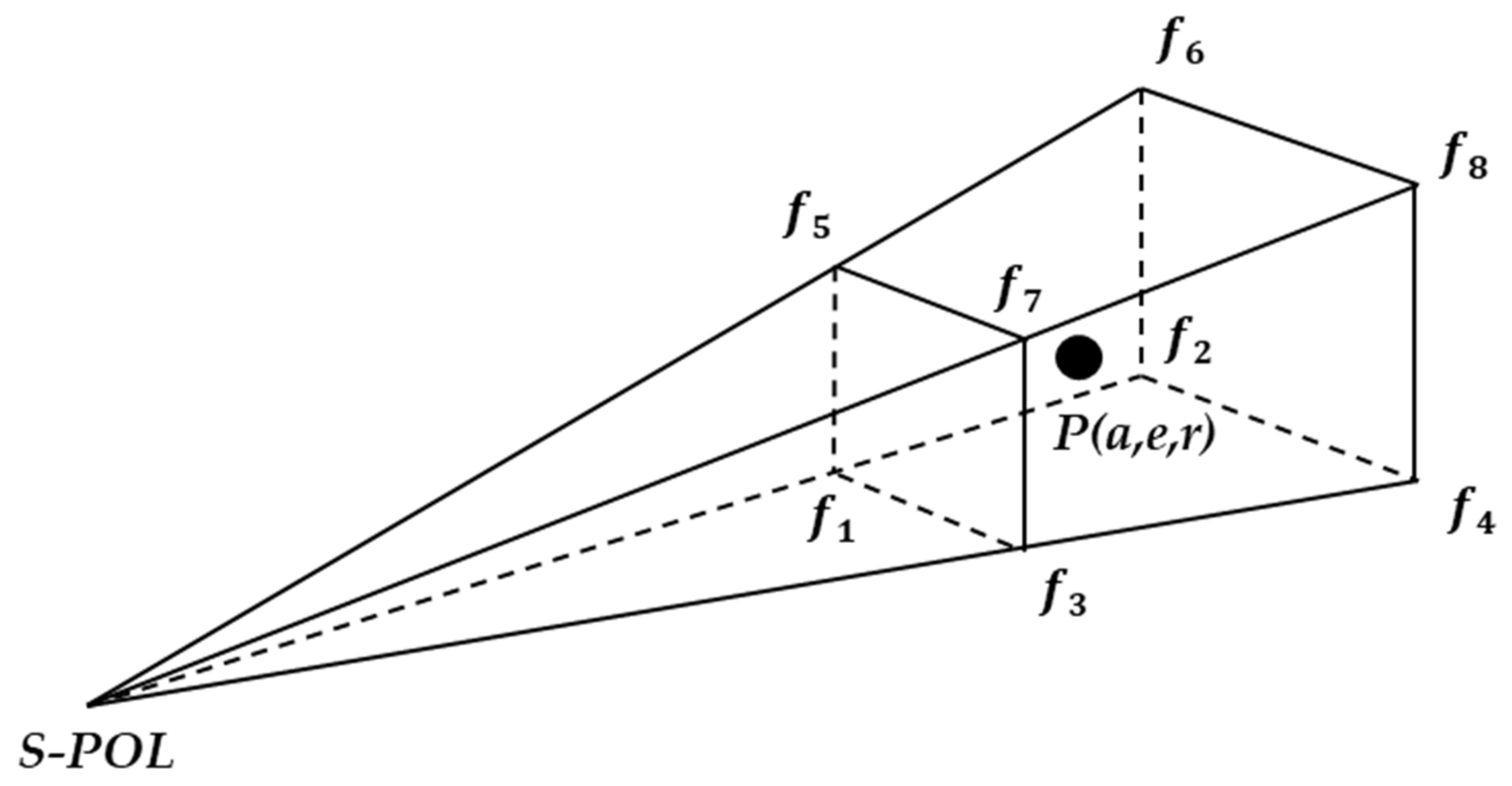
2.4.2. Interpolation Matching of X-PAR and S-POL and Calculation of System Bias

In this paper, the S-POL observation data were used to calculate the X-PAR system bias and attenuation-correction parameters (Figure 3), and to test the attenuation-correction results. The spatial and temporal resolutions of X-PAR and S-POL differ, so it is necessary to match the observation gates. The reflectivity of S-POL at the coordinates of X-PAR can be obtained via the eight-gate interpolation method. Firstly, the X-PAR observation gate P is transformed into S-POL coordinates (a, e, r), where a is the azimuth angle, e is the elevation angle, and r is the radial distance.
Eight gates— f 1 a 1 , e 1 , r 1 , f 2 a 1 , e 1 , r 2 , f 3 a 2 , e 1 , r 1 , f 4 a 2 , e 1 , r 2 , f 5 a 1 , e 2 , r 1 , f 6 a 1 , e 2 , r 2 , f 7 a 2 , e 2 , r 1 , and f 8 a 2 , e 2 , r 2 —are taken in the coordinate of the S-POL, where a1 and a2, e1 and e2, and r1 and r2 are adjacent coordinates, with a1 < a < a2, e1 < e < e2, r1 < r < r2. f a , e , r t as the interpolation result of S-POL at X-PAR observation gate P, and f a , e , r t can be calculated by Equation (18):
f a , e , r t = w e 1 w a 1 w r 1 f 1 + w r 2 f 2 + w a 2 w r 1 f 3 + w r 2 f 4 + w e 2 w a 1 w r 1 f 5 + w r 2 f 6 + w a 2 w r 1 f 7 + w r 2 f 8
where w is the interpolation weight.
w a 1 = a 2 a / a 2 a 1 w a 2 = a a 1 / a 2 a 1 w e 1 = e 2 e / e 2 e 1 w e 2 = e e 1 / e 2 e 1 w r 1 = r 2 r / r 2 r 1 w r 2 = r r 1 / r 2 r 1
It is noted that the interpolation of the low-resolution S-POL data into high-resolution data inevitably involves the loss of the detailed features of the echo structure. However, each parameter calculated using S-POL interpolation data depends on the statistical results of a large number of data, and the negative impact of the lack of detail caused by interpolation in this statistical calculation is tolerable. In addition, S-POL is different from the X-PAR scanning system; there is a big difference in temporal resolution. The corresponding time of the elevation angle with greater spatial-interpolation weight is set to be the time of the interpolation result, and the observation that the X-PAR scan that is closest in time to the interpolation time is used. For example, for one gate P, ZSX0 interpolated by S-POL includes elevation1 (corresponding to scan time t1) and elevation2 (scan time t2). If the data of elevation1 has more weight in interpolation, then the interpolation time TS of S-POL at gate P is t1 and vice versa. The observation time of the scans of X-PAR at gate P are t1x, t2x, …tnx, and the case that is closest to TS is taken as ZX0 from X-PAR.
Through the band conversion and space interpolation of the S-POL reflectivity and under the assumption that the gates with φ D P < 5° of X-PAR are less affected by attenuation, ZSX0 and ZX0 are fitted using the least squares and the following Equation (19):
Z X 0 = Z S X 0 + b i a s
where Z X 0 is the reflectivity (dB) of X-PAR; Z S X 0 is the reflectivity (dB) of S-POL under the process of band conversion from S-band to X-band and the space interpolation from S-POL to X-PAR; and the intercept is the system bias. According to Equation (20), the reflectivity of the S-band radar matching the X-PAR can be obtained, which is the Z S X used for the calculation of γ1 and γ2 and the test of attenuation correction effect.
Z S X = Z S X 0 + b i a s

2.4.3. Estimation of γ1 and γ2

As mentioned above, γ1 and γ2, which minimize the difference between γ 1 Δ φ D P 1 + γ 2 Δ φ D P 2 and Z S X r m Z X 0 r m , are the optimal attenuation-correction parameters, which can be obtained by solving a linear-programming (LP) problem.
For a PPI scan, there are n ray paths for precipitation data. Based on the precipitation classification, the two-way propagation differential phase of weak rainfall is Δ φ D P 1 = Δ φ D P 11 , Δ φ D P 12 Δ φ D P 1 n , the two-way propagation differential phase of heavy rainfall is Δ φ D P 2 = Δ φ D P 21 , Δ φ D P 22 Δ φ D P 2 n , and the PIA of each ray path is
P I A i = Z S X i Z X 0 i
where ZX0i (unit: dB) is the reflectivity at the end (rainfall area) of i-th ray path of the X-PAR, and Z S X i (unit: dB) is the corresponding reflectivity converted from S-POL to X-PAR.
Although the system bias is corrected, factors such as different scan mode and interpolation still introduce errors into the PIA. However, such errors are limited. Especially when electromagnetic waves pass through large-scale precipitation, the proportion of these errors in PIA decrease accordingly. Therefore, the weight coefficient wi should be brought in to assign greater weight to Δ φ D P i with a large value on the ray path.
w i = Δ φ D P 1 i + Δ φ D P 2 i 1 n Δ φ D P 1 i + Δ φ D P 2 i
The cost function is defined as L = i = 1 n w i γ 1 Δ Φ D P 1 i + γ 2 Δ Φ D P 2 i P I A i . The optimum γ1 and γ2 are those that make L lowest. Non-negative x i is brought in, such that:
γ 1 Δ φ D P 1 i + γ 2 Δ φ D P 2 i P I A i x i
Minimizing L can be transformed into minimizing i = 1 n w i x i , and Equation (23) can be equivalently transformed into:
x i + γ 1 Δ φ D P 1 i + γ 2 Δ φ D P 2 i P I A i
x i γ 1 Δ φ D P 1 i γ 2 Δ φ D P 2 i P I A i
The following is set up:
x c = γ 1 , γ 2 , x 1 , x 2 , x 3 x n
M = 1 1 , 0 2 , 0 3 0 n 0 1 , 1 2 , 0 3 0 n 0 1 , 0 2 , 1 3 0 n 0 1 , 0 2 , 0 3 1 n
A = Δ φ D P 1 T ,   Δ φ D P 2 T ,   M Δ φ D P 1 T , Δ φ D P 2 T , M
b = P I A T P I A T
Equation (23) can be converted to matrix form A xc b.
With the weight coefficient, row-matrix c is introduced:
c = 0 , 0 , w 1 , w 2 , w 3 w n
The i = 1 n w i x i minimization can be transformed into the minimization of c · xc.
Then, estimating γ1 and γ2 can be transformed into solving a linear-programming problem as follows:
Minimizec · xc
Subject toA xcb
x c z , x T 0
By solving the linear-programming problem, x c can be obtained, and then γ1 and γ2 can be obtained. Next, γ1 and γ2 are substituted into Equation (9) so that the AH of each gate on the ray path can be obtained; then, the attenuation corrected reflectivity can be calculated by Equation (12).

3. Results

3.1. Analysis of the DSD Measurement

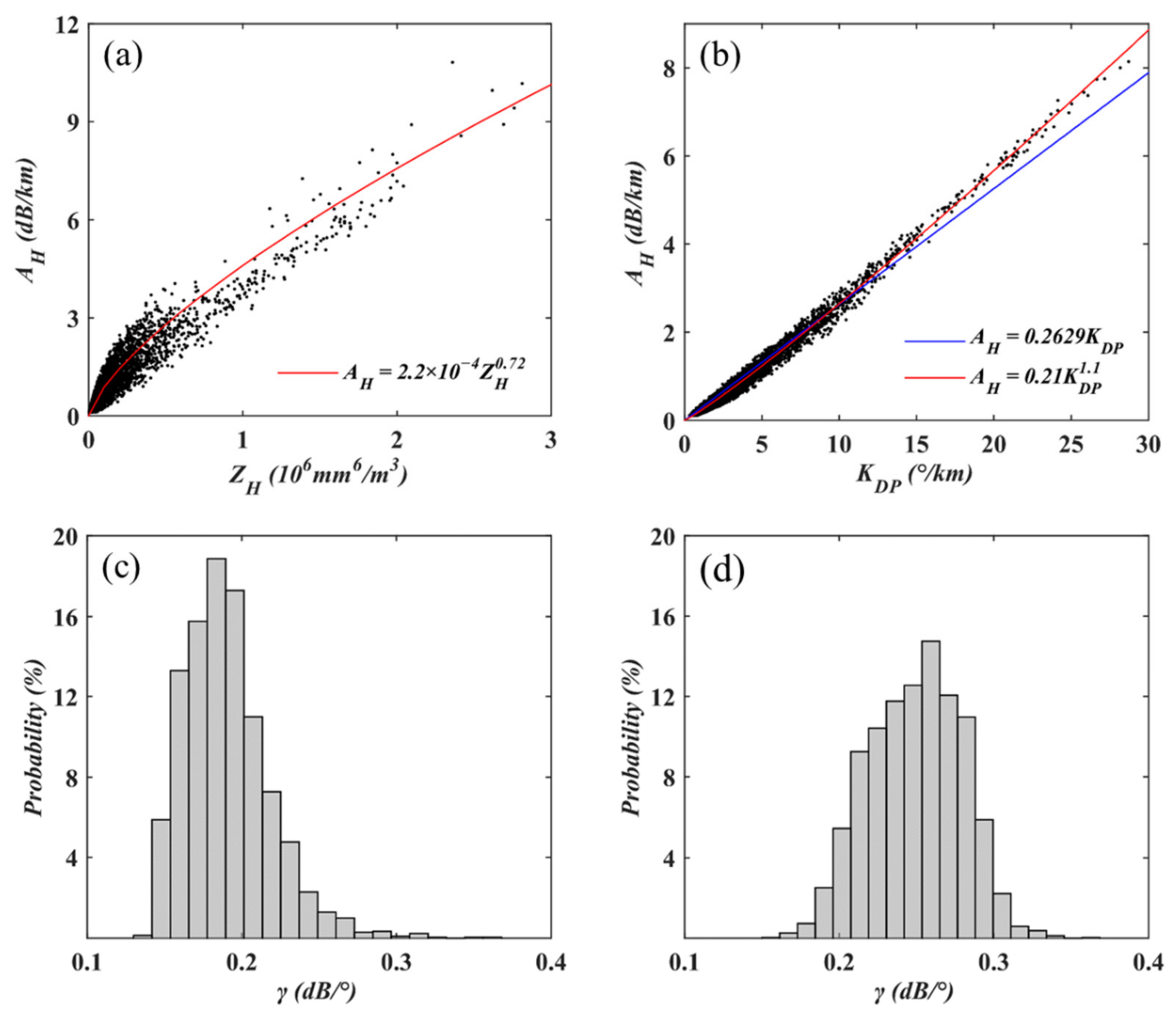
3.1.1. Statistic Analysis of the Variables Simulated from DSD Measurement

Based on the DSD measurement of Longmen from April 2019 to April 2022, there was an exponential relationship between AH and ZH (as shown in Figure 4a), and the power-exponent b was 0.72. AH and KDP had an exponential relationship (as shown in Figure 4b), and the power-exponent β was 1.1, so it can be assumed that AH = γKDP. Based on this quasi-linear relationship, a simple φDP integral attenuation calculation can be realized. It is worth noting that when the KDP was large, the error between the AH calculated with the linear relationship and the actual AH gradually increased, which brought errors into the PIA, especially when the radar’s electromagnetic wave passed through continuous strong rainfall. Considering that γ varies due to differences in the physical characteristics of raindrops, the γ was calculated according to the linear relationship of AHKDP for weak rainfall (<45 dBZ) and heavy rainfall (>45 dBZ). The results showed that the expected value of γ for weak rainfall (as shown in Figure 4c) was 0.19, and the expected value of γ for heavy rainfall (as shown in Figure 4d) was 0.25. γ in the heavy-rainfall area was higher than that in the weak-rainfall area, which is basically consistent with previous research [10]. According to the probability distribution of γ, the γ of heavy rainfall was mainly distributed at 0.2–0.3 dB/°. For a heavy precipitation with φDP > 100°, the different γ could create attenuation correction on the end of the ray path with a difference of more than 10 dBZ.

3.1.2. Case Study of the Variables Simulated by DSD Measurement

The strongest continuous precipitation process (20:30 on 8 June 2020 to 01:30 UTC the next day) from the measurement data was taken as an example to analyze the time-series variation characteristics of AH, ZH, and γ (as shown in Figure 5). For relatively strong precipitation periods, such as 21:10–21:30 and 21:50–22:00, the attenuation was larger than that before 21:00, and the γ was generally stable at about 0.25 dB/°. After 22:00, there was a period of continuous heavy rainfall. Although AH and ZH fluctuated greatly with time, γ was generally stable at about 0.3 dB/°. In this case, the main attenuation came from the continuous heavy rainfall after 22:00, and γ in this condition was relatively stable; the γ of the weak rainfall before 22:00 was smaller than that of the heavy rainfall, and the fluctuation was more severe. However, the attenuation before 22:00 was underweight in the overall attenuation. Therefore, setting one appropriate γ for the weak-rainfall section did not introduce much error into the attenuation correction.
Thus, for the attenuation correction in the following, according to the precipitation intensity classification, two γ values could be used for attenuation calculation, setting γ1 for the non-continuous heavy rainfall with large fluctuations (or weak precipitation) and γ2 for the continuous heavy rainfall. In this way, the influence of differences in precipitation types was taken into account, and the calculating amount did not need to be increased excessively.

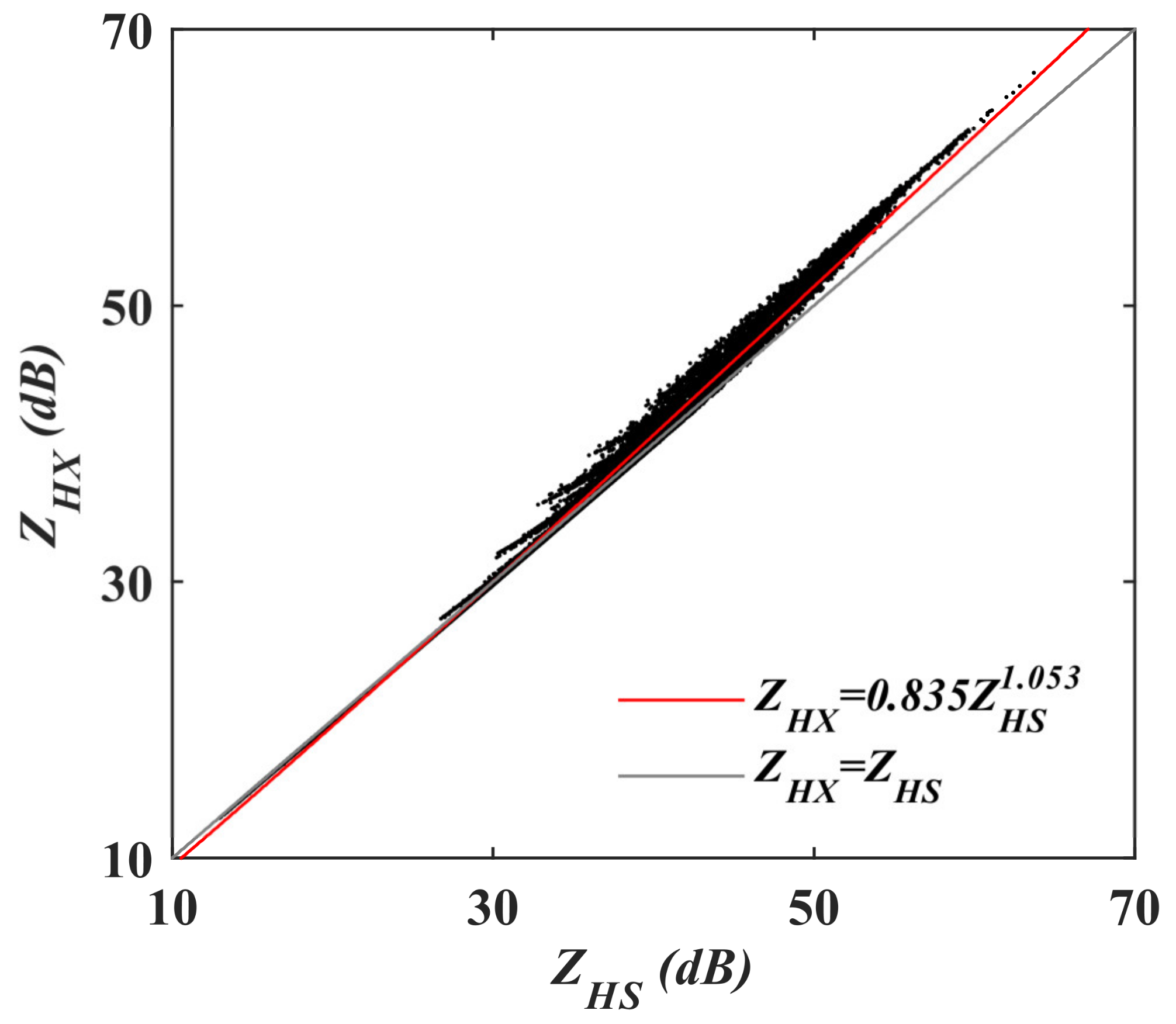
3.1.3. Fitting Relationship between S- and X-Band Reflectivity Based on DSD Data

The reflectivity of X- and S-bands were calculated using the DSD measurement data. For the two bands, the Rayleigh scattering assumption was valid for the weak rainfall, and the reflectivity showed a good linear relationship. As the particle size increased, the assumption of the Rayleigh scattering was no longer valid for both bands, and the reflectivity distributions of the two bands became scattering (as shown in Figure 6).
Based on the assumption of an exponential relationship, the reflectivity of the two wavelengths was fitted to obtain the equation ZHX = 0.835ZHS1.053 (unit: dB), where the fitting coefficient of determination was 0.9974. Through the statistical fitting, the root-mean-square error was 0.46 dB and the deviation within 1 dB accounted for 95.94%. If there was no fitting, the root-mean-square error was 0.70 dB and the deviation within 1 dB accounted for 89.78%. Overall, a well-fitting effect was achieved.

3.2. Case Analysis of Attenuation Correction for X-PAR

From 01:00 to 03:00 on 5 June 2020, there was convective weather within the observation range of X-PAR1, and the echo moved along in a southwest–northeast direction. According to the attenuation-correction method described in Section 2.4, an example from 01:44 to 01:50 (UTC) was taken for analysis. The radar-observation data within 1 h before 01:44 were used to calculate the system bias and attenuation-correction parameters γ1 and γ2 for the attenuation correction of the X-PAR reflectivity from 01:44 to 01:50. Furthermore, the S-POL data corresponding to 01:50 were taken to test the results of the attenuation correction.

3.2.1. The Calculation of PIA

According to the correction method described in Section 2.4, attenuation correction at the target time 01:50 was achieved through the following steps:
  • ΦDP preprocessing and preliminary attenuation correction for the observation within 1 h before the target time (only observation at 01:44 was shown in Figure 7a–c) to obtain precipitation classification (Figure 7a) and φDP (Figure 7b).
  • PIA0 as the difference between ZSX from S-POL and ZX0 (without attenuation correction) from X-PAR (Figure 7c).
  • γ1 and γ2 calculated by the algorithm described in Section 2.4.3 using PIA0, φDP, and precipitation classification.
  • ΦDP preprocessing and preliminary attenuation correction for the observation at the target time to obtain precipitation classification (Figure 7d) and φDP (Figure 7e).
  • According to Equations (9) and (12) and using γ1, γ2, φDP, and precipitation classification, PIAt (Figure 7f) was obtained for attenuation correction at the target time.
Due to the differences in the spatio-temporal resolutions of S-POL and X-PAR, the PIA0 could not strictly and monotonously increase on the ray path (as shown in Figure 7c). However, the error caused by the mismatching could be suppressed by the statistics of the whole of the scanning data; the calculated PIAt could strictly and monotonously increase along on the ray path and was basically similar to the PIA0 structure of the previous time. The method proposed in this paper obtained a relatively stable and reasonable PIA.

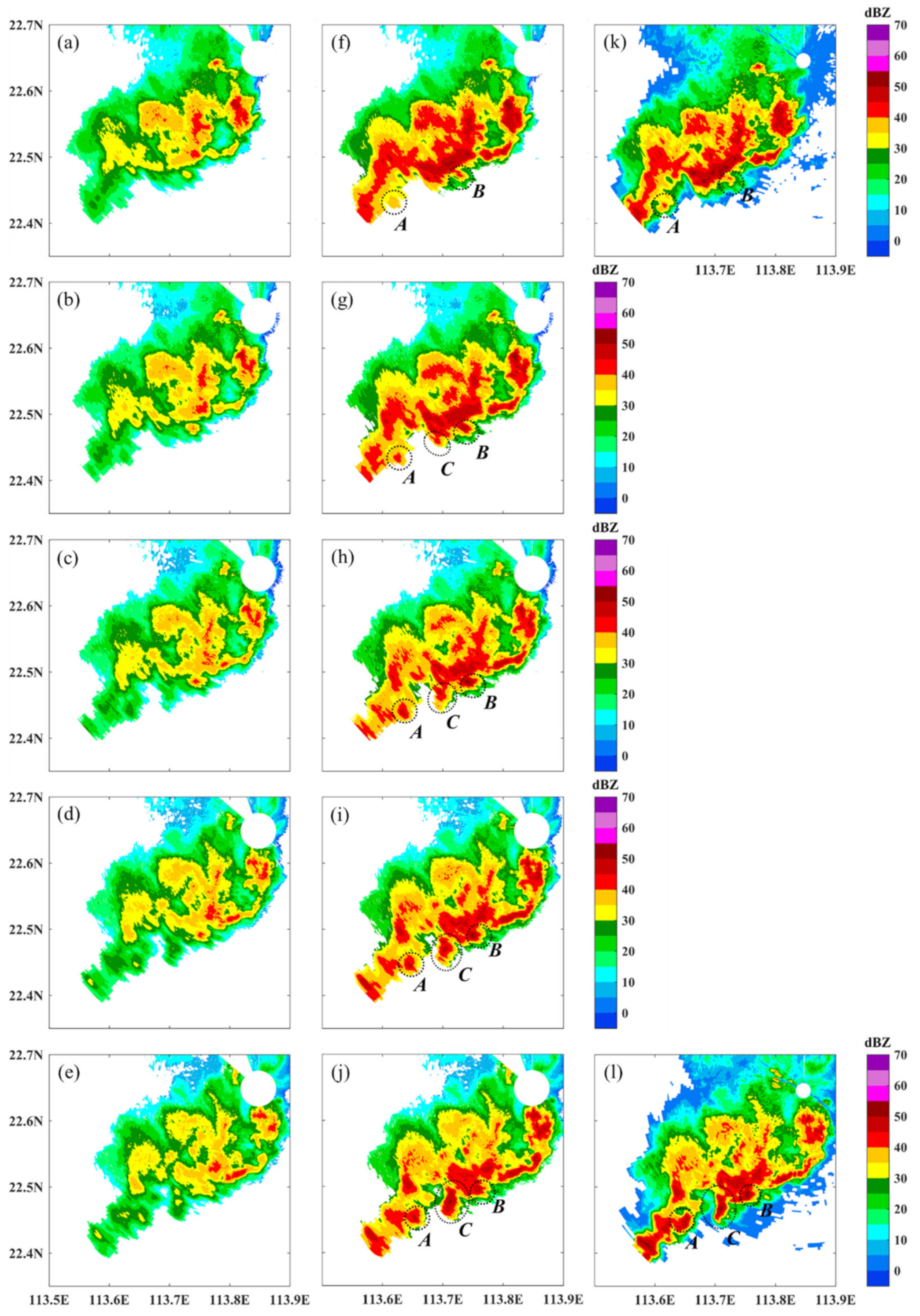
3.2.2. PPI Reflectivity Analysis

Using the γ1 and γ2 calculated in Section 3.2.1, attenuation correction was performed on the reflectivity of the X-PAR at an elevation angle of 4.5° from 01:44 to 01:50, as shown in Figure 8, where Figure 8a–e is the reflectivity of the X-PAR at 01:44 to 01:50 before attenuation correction and Figure 8f–j is the attenuation-corrected X-PAR reflectivity. Figure 8k,l is the ZSX at 01:42 and 01:48, respectively (with the conversion from S-band to X-band, system-bias correction, and time matching).
The attenuation-corrected reflectivity structure of the X-PAR was consistent with that of the S-POL data at 01:44 and 01:50. Being affected by attenuation, the strong convective echo at the far end of path ray was attenuated to only 15–20 dBZ. The magnitude of the corrected echo far from the X-PAR was consistent with that of the S-POL, and there was no obvious overcorrection.
Although the interval between the two S-POL scans was only 6 min, there were still obvious echo evolutions. For example, cells A and B were at the edge of the strong echo of the main body at 01:44. Nevertheless, after 6 min, cells A and B were difficult to identify. Based on the attenuation-corrected X-PAR observation, cell A continuously strengthened within 6 min and moved to a new position in a southwest–northeast direction, whereas cell B experienced an enhancement-merging process with the main-body echo. Additionally, C cell was not visible in the S-POL at 01:44, but it reached a very strong magnitude at 01:50.
The evolution of the three cells mentioned above could not be observed via the S-POL with a low time resolution or via the X-PAR without attenuation correction. It could only be observed by the X-PAR under stringent quality controls.
This first proves the stability of the X-PAR attenuation correction method, which can promote echo-evolution information. Second, this proves that X-PAR networked with S-POL can supplement the evolution information of the precipitation system.
The difference between Figure 8j,l that mainly manifested in the strong echo far from X-PAR had a larger distribution range in the azimuth than did S-POL, but its magnitude was weaker than that of S-POL, such as cell C near (22.4°N, 113.6°E); however, this phenomenon was relatively inconspicuous near the radar. This is because the X-PAR beamwidth was wider and the resolution of the azimuth was lower. There was a relatively obvious smoothing effect in the azimuth direction, particularly for echoes far from X-PAR.

3.2.3. Error Analysis

The frequency plots after matching the reflectivity of the X-PAR and S-POL at 01:50 are shown in Figure 9, Figure 9a,b shows the comparison between the X-PAR reflectivity before (ZX0) and after (ZXC) the correction, respectively, and the S-POL-converted reflectivity (ZSX). There were many ZX0 deviating from ZSX (as shown in Figure 9a); however, the correlation between ZXC and ZSX was obviously improved upon attenuation correction (as shown in Figure 9b).
For the frequency plots of φDP > 40° for X-PAR and S-POL (as shown in Figure 9c,d), the ZX0 was significantly underestimated due to the attenuation. The deviation between ZXC and ZSX was improved after the correction. It should be noted that ZXC was overestimated for the relatively low part of ZSX (<40 dBZ), whereas it was underestimated for the relatively high part of ZSX (>40 dBZ). One may be due to the wide beamwidth of X-PAR, which over-smoothed the reflectivity of the X-PAR at the azimuth direction.

3.2.4. Self-Consistency Analysis

According to the statistical results of the DSD data in Section 3.1.1, there was an exponential relationship between ZH (unit: mm6/m3) and AH (unit: dB/km). As shown in Figure 10a, the distribution of ZX0 and AH was scattering, which deviated from the DSD fitting result (gray curve). By contrast, the distribution of ZXC and AH were closer to the DSD fitting result.
A similar analysis was performed on the gates with φDP > 40° (Figure 10c,d), and the ZX0 deviated far from the DSD fitting results, whereas the distribution of ZXC and AH with φDP > 40° was similar to that in Figure 10b, which is basically consistent with the DSD fitting results. The attenuation-correction method used in this paper ensured the self-consistency between AH and the ZH, leading to reasonable attenuation correction.
It should be noted that the DSD fitting results based on historical statistics are used as a reference to check the self-consistency of the attenuation-corrected polarimetric variables. However, the test of attenuation correction in this section is a case analysis. As described in 2.3, a is a variable parameter in AH = aZb. Therefore, a small deviation between the distribution of ZXC and AH and the DSD fitting results of historical statistics is acceptable.
This case analysis showed that the attenuation-correction method can be used to calculate the stable and reasonable values of AH, ZH, and PIA. Moreover, the high time resolution of X-PAR made it possible to accurately observe the evolution of weather systems. The attenuation-corrected reflectivity of X-PAR was consistent with that of the S-POL. Limited by beam broadening, the reflectivity magnitude was smooth in the azimuth direction, especially the echo far from the radar.

3.3. Statistical Test

3.3.1. Case Selection

In order to further verify the effect of the attenuation-correction method proposed in this paper, the consistency of the reflectivity from X-PAR and S-POL deployed in the network was checked. We selected the cases with large-scale strong rainfall observed by the two X-PARs in 2020 (as shown in Table 2). To test the effect of proposed method, the previous classical methods were used to correct attenuation for the same case, and deviations among the corrections of different methods were compared.

3.3.2. Comparison Experiments

For the two X-PARs, three groups of data and five experiments for the attenuation correction of the reflectivity were designed. The three groups of data were categorized as follows:
  • The data of all the gates within the X-PAR detection range, which were used to represent the overall attenuation-correction results.
  • The data of the gates with ZSX0 > 45 dB, which were used to represent the attenuation-correction results in heavy rainfall.
  • The data of the gates with φ D P > 4 0°, which were used to represent the attenuation-correction results in strong attenuation area.
The five attenuation-correction experiments were designed as follows:
  • Exp0: The measured reflectivity of X-PAR without attenuation correction.
  • Exp1: Based on constant γ, the PIA was calculated through the DP method, that is, using the fitting γ obtained according to Section 3.1.1, and attenuation correction was performed with Equations (7) and (8).
  • Exp2: To calculate γ1 and γ2 based on precipitation classification, and then the PIA was calculated using φ D P ; that is, γ1 and γ2 were calculated according to Section 2.4.3, and attenuation correction was performed with Equations (7) and (8).
  • Exp3: Based on constant γ and the ZPHI method, AH was calculated for attenuation correction; that is, using the fitting γ obtained according to Section 3.1.1, and attenuation correction was performed with Equations (9) and (12).
  • Exp4: To calculate γ1 and γ2 based on precipitation classification, and the AH was calculated based on the ZPHI method for attenuation correction; that is, γ1 and γ2 were calculated according to Section 2.4.3, and attenuation correction was performed with Equations (9) and (12).
  • Exp5: The AH was calculated using the self-consistent method for attenuation correction; that is, calculating the optimal solution of γ for each ray path by Equations (13) and (14), and then combing with Equations (9) and (12) to perform attenuation correction.
The differences between the five methods are mainly in the estimation of γ and the calculation of AH (or PIA). Table 3 provides a brief summary of these experiments.
Using the experiment scheme above, the mean value of ZSX0, ZX-bias, mean deviation (MD), mean absolute deviation (MAD), root-mean-square difference (RMSD), and correlation coefficient (R) could be calculated.
MD = ( Z S X Z X ) N
MAD = Z S X Z X N
RMSD = Z S X Z X 2 N
where N is the observed gate number of all volume-scan data, and the unit of ZSX and ZX is dB.
In order to show the effect of the attenuation-correction method in individual cases, the correlation coefficient R in this paper is the weighted average of the correlation coefficient r calculated for each volume scan. That is, the correlation coefficient ri of each volume-scan data point is calculated, and then R is calculated by using the weighted-average method.
r i = Z X Z X ¯ Z S X Z S X ¯ Z X Z X ¯ 2 Z S X Z S X ¯ 2
R = n i r i N
where ni is the observed gate number of the i-th volume-scan data.

3.3.3. Deviation Statistics

Table 4 and Table 5 show the statistical results of the reflectivity before and after the attenuation correction for the two X-PARs, and the deviation of the reflectivity after correction by the five methods was significantly improved.
Compared with the constant γ correction method, the attenuation-correction method proposed in this paper did not significantly improve the deviations of all the gates and even slightly increased some of them. However, for the heavy-rainfall area (ZSX0 > 45 dB) and the rain area after strong attenuation (φDP > 40°), the deviations were obviously reduced. For the statistical results, the improved method had little negative impact on the overall deviation, whereas the improvement in the corrections for the strong echo and the observation after strong attenuation were obvious.
For the constant γ, the attenuation correction of the ZPHI method (Exp3) was superior to that of the DP method (Exp1) overall. After the classified calculation of γ, the corrections of the ZPHI (Exp4) and DP method (Exp2) were basically the same, which shows that our γ calculation method more obviously improved the DP method. The main reason for this is that, for the DP method, the PIA of each gate on the ray path depends on the accuracy of γ and φDP. The improvement in the accuracy of γ had a more obvious beneficial effect on the final attenuation-correction result of the DP method than that of the ZPHI method.
The MD calculated after attenuation correction in the heavy-precipitation area (ZSX0 > 45 dB) was generally larger, which may have been due to the temporal–spatial mismatching of S-POL and X-PAR. For the area that was relatively continuous with small spatial gradients, the impact of the mismatching on the deviation was limited. By contrast, the area of strong echo was generally smaller than the area of large-scale stable weak rainfall. The large horizontal gradient of the reflectivity in the strong-echo areas increased the influence of mismatching on the deviation. Furthermore, the self-consistent method was superior to other methods in the strong-echo area (ZSX0 > 45 dB) because the heavy-rainfall area had a larger AH and KDP, which was beneficial to obtain a stable and accurate optimal γ solution. However, the solution of γ was unstable for the weak-rainfall in many areas, which is adverse for attenuation correction. Thus, the deviation of the self-consistent method for all the gates and φDP > 40° was generally lager than that of other methods.
The deviations of the two X-PARs were basically the same. However, the correlation between X-PAR1 and S-POL was higher than that of X-PAR2 and S-POL in the heavy-rainfall area and the rainfall area after strong attenuation. This is because S-POL and X-PAR1 were in the same location, whereas S-POL and X-PAR2 were about 70 km apart; due to the effects of beam broadening, the spatial resolution of S-POL in the X-PAR2 coverage was lower than that in the X-PAR1 coverage.

4. Discussion

Upon using an OTT PARSIVEL laser disdrometer DSD to simulate and calculate the ZH, KDP, and AH of an X-band weather radar, AH and KDP presented a good quasi-linear relationship, and the proportional coefficient γ of the two differed with the distribution of heavy and weak rainfall. The case analysis showed that there was a stable γ during a period of continuous heavy rainfall and relatively strong fluctuations in γ during a period of rainfall-intensity fluctuations. However, during the entire rainfall period, the attenuation of continuous heavy rainfall was much stronger than that of the rainfall with strong fluctuations. In attenuation-correction processing, the precipitation system could be classified into two parts—weak rainfall and continuous heavy rainfall—and the optimal γ for each type of precipitation could be calculated for attenuation correction.
Under the temporal and spatial matching, wavelength conversion and system-bias correction of S-POL and X-PAR, and the assumption that S-POL was less affected by precipitation attenuation, the PIA of X-PAR could be obtained. The γ1 for weak rainfall and the γ2 for heavy rainfall could be calculated by linear programming. The ZPHI or DP method could then be used to calculate the AH or PIA to correct the precipitation attenuation of X-PAR. The echo structure and intensity of the X-PAR reflectivity via our corrected method were basically consistent with those of S-POL. This case analysis shows that both S-POL data with low temporal resolution and X-PAR data without attenuation correction make it difficult to observe the fine evolution characteristics of convective cells. Nevertheless, X-PAR data after attenuation correction observed a fine and continuous echo evolution, including changes such as the enhancement and merging of echoes with relatively small spatial scales. The corrected ZH and calculated AH were close to the statistical relationship based on the disdrometer DSD data, which was a self-consistent corrected result. The disadvantage of the X-PAR attenuation-corrected reflectivity was that its horizontal beamwidth was very wide, which resulted in the over-smoothness of reflectivity at the azimuth direction, especially the observation far from the radar. Given the limitations of radar hardware, it is expected that this adverse effect would be reduced by the use of a multiple-radar network mosaic.
The effect of the improved attenuation-correction method was compared with that of the previous classical methods. The results showed that this method can effectively realize the attenuation correction for X-PAR. Even for the area with φDP > 40°, it could also achieve high correlation and less deviation with S-POL. With S-POL as the constraint, attenuation correction by precipitation classification was better than the method based on constant γ, and the improvement effect of the γ classification calculation on the DP method was more obvious than that on the ZHPI method. The attenuation-correction results of the self-consistent method were superior in the heavy-rainfall area, but the results of the rainfall area after strong attenuation were not as good as those of other methods.
It should be noted that the difference in beam width and spatial–temporal resolution of X-PAR and S-POL might exacerbate the mismatching between the observation of two radars in same atmospheric volume. However, the estimation of γ1 and γ2 were statistical results of the whole of the scanning data, and a sufficient sample size could suppress the impact of mismatching. Therefore, our method is suitable for large-scale precipitation systems, which provide more observation samples, rather than an independent small-scale convective system. For small-scale convective precipitation, the attenuation is generally not serious, and it is acceptable and reasonable to use the constant γ for attenuation correction.
For precipitation classification, we distinguished between heavy and weak precipitation simply according to the preliminary attenuation-correction reflectivity. However, the linear-programming method supports more precipitation classification schemes, which may improve the estimation of γ for the different precipitation types. Note that more precipitation classification means a larger sample-size requirement. Under a limited sample size, too many precipitation classifications may lead to an unreasonable estimation of γ.
Overall, the improved method could obtain an X-PAR attenuation correction that is more consistent with S-POL observations. This study proves the effect of the attenuation-correction method based on multi-band radar network and precipitation classification, and showed that although the X-PAR and S-POL set in South China differed in wavelength, scan mode, and beam width, under stringent quality control, a consistent observation could still be obtained. The observation of X-PARs with high temporal and spatial resolutions are expected to form accurate radar-observation fields, and may further realize multi-radar mosaic with an S-POL radar network.

Author Contributions

Conceptualization, L.L.; methodology, F.G. and L.L.; software, F.G. and L.L.; validation, F.G.; formal analysis, F.G.; investigation, F.G. and L.L.; resources, L.L.; data curation, F.G.; writing—original draft preparation, F.G.; writing—review and editing, F.G.; visualization, F.G.; supervision, L.L.; project administration, L.L.; funding acquisition, L.L. All authors have read and agreed to the published version of the manuscript.

Funding

This research was funded by the National Natural Science Foundation of China (Grant No. U2142210).

Data Availability Statement

Not applicable.

Conflicts of Interest

The authors declare no conflict of interest.

References

  1. Wu, C.; Liu, L.; Liu, X.; Li, G.; Chen, C. Advances in Chinese dual-polarization and phased-array weather radars: Observational analysis of a supercell in southern China. J. Atmos. Ocean. Technol. 2018, 35, 1785–1806. [Google Scholar] [CrossRef]
  2. Zhao, G.; Huang, H.; Yu, Y.; Zhao, K.; Yang, Z.; Chen, G.; Zhang, Y. Study on the quantitative precipitation estimation of X-band dual-polarization phased array radar from specific differential phase. Remote Sens. 2023, 15, 359. [Google Scholar] [CrossRef]
  3. Bringi, V.N.; Chandrasekar, V.; Balakrishnan, N.; Zrnic, D. An examination of propagation effects in rainfall on radar measurements at microwave frequencies. J. Atmos. Ocean. Technol. 1990, 7, 829–840. [Google Scholar] [CrossRef]
  4. Testud, J.; Bouar, E.L.; OBligis, E.; Ali-Mehenni, M. The rain profiling algorithm applied to polarimetric weather radar. J. Atmos. Ocean. Technol. 2000, 17, 332–356. [Google Scholar] [CrossRef]
  5. Matrosov, S.Y. Evaluating polarimetric X-band radar rainfall estimators during HMT. J. Atmos. Ocean. Technol. 2010, 27, 122–134. [Google Scholar] [CrossRef]
  6. Park, S.G.; Bringi, V.N.; Chandrasekar, V.; Maki, M.; Iwanami, K. Correction of radar reflectivity and differential reflectivity for rain attenuation at X band. Part I: Theoretical and empirical basis. J. Atmos. Ocean. Technol. 2005, 22, 1621–1632. [Google Scholar] [CrossRef] [Green Version]
  7. Park, S.G.; Maki, M.; Iwanami, K.; Bringi, V.N.; Chandrasekar, V. Correction of radar reflectivity and differential reflectivity for rain attenuation at x band. Part II: Evaluation and application. J. Atmos. Ocean. Technol. 2005, 22, 1633–1655. [Google Scholar] [CrossRef]
  8. Matrosov, S.Y.; Clark, K.A.; Martner, B.E.; Tokay, A. X-band polarimetric radar measurements of rainfall. J. Appl. Meteorol. 2002, 41, 941–952. [Google Scholar] [CrossRef]
  9. Bringi, V.N.; Keenan, T.; Chandrasekar, V. Correcting c-band radar reflectivity and differential reflectivity data for rain attenuation: A self-consistent method with constraints. Geosci. Remote Sens. IEEE Trans. 2001, 39, 1906–1915. [Google Scholar] [CrossRef]
  10. Kim, D.S.; Maki, M.; Lee, D.I. Correction of X-band radar reflectivity and differential reflectivity for rain attenuation using differential phase. Atmos. Res. 2008, 90, 1–9. [Google Scholar] [CrossRef]
  11. Kim, D.S.; Maki, M.; Lee, D.I. Retrieval of three-dimensional raindrop size distribution using x-band polarimetric radar data. J. Atmos. Ocean. Technol. 2010, 27, 1265–1285. [Google Scholar] [CrossRef]
  12. Gorgucci, E.; Chandrasekar, V.; Baldini, L. Correction of x-band radar observation for propagation effects based on the self-consistency principle. J. Atmos. Ocean. Technol. 2006, 23, 1668–1681. [Google Scholar] [CrossRef] [Green Version]
  13. Gu, J.Y.; Ryzhkov, A.; Zhang, P.; Neilley, P.; Knight, M.; Wolf, B.; Lee, D.I. Polarimetric attenuation correction in heavy rain at C band. J. Appl. Meteorol. Climatol. 2011, 50, 39–58. [Google Scholar] [CrossRef]
  14. Scarchilli, G.; Gorgucci, V.; Chandrasekar, V.; Abdullah, D. Self-consistency of polarization diversity measurement of rainfall. IEEE Trans. Geosci. Remote Sens. 1996, 34, 22–26. [Google Scholar] [CrossRef] [Green Version]
  15. Chandrasekar, V.; Lim, S. Retrieval of Reflectivity in a Networked Radar Environment. J. Atmos. Ocean. Technol. 2008, 25, 1755–1767. [Google Scholar] [CrossRef]
  16. Lim, S.; Chandrasekar, V.; Wang, Y. A network based attenuation correction system for networked dual polarization radar observations. In Proceedings of the 2010 IEEE International Geoscience and Remote Sensing Symposium, Honolulu, HI, USA, 25–30 July 2010; pp. 2333–2336. [Google Scholar] [CrossRef]
  17. Cruz-Pol, S.; Mora, K.; Leon, L. Implementation and development of an attenuation correction algorithm for off-the-grid x-band radar network. In Proceedings of the 93rd American Meteorological Society Annual Meeting, San Juan, PR, USA, 1 January 2013. [Google Scholar]
  18. Lengfeld, K.; Clemens, M.; Merker, C.; Münster, H.; Ament, F. A simple method for attenuation correction in local x-band radar measurements using c-band radar data. J. Atmos. Ocean. Technol. 2016, 33, 2315–2329. [Google Scholar] [CrossRef]
  19. Wang, C.; Wu, C.; Liu, L.; Liu, X.; Chen, C. Integrated correction algorithm for x band dual-polarization radar reflectivity based on cinrad/sa radar. Atmosphere 2020, 11, 119. [Google Scholar] [CrossRef] [Green Version]
  20. Wu, Y.; Liu, L. Statistical characteristics of raindrop size distribution in the Tibetan Plateau and southern China. Adv. Atmos. Sci. 2017, 34, 727–736. [Google Scholar] [CrossRef]
  21. Tokay, A.; Petersen, W.A.; Gatlin, P.; Wingo, M. Comparison of raindrop size distribution measurements by collocated disdrometers. J. Atmos. Ocean. Technol. 2013, 30, 1672–1690. [Google Scholar] [CrossRef]
  22. Jaffrain, J.; Berne, A. Experimental quantification of the sampling uncertainty associated with measurements from parsivel disdrometers. J. Hydrometeorol. 2011, 12, 352–370. [Google Scholar] [CrossRef]
  23. Pruppacher, H.; Beard, K. A wind tunnel investigation of the internal circulation and shape of water drop falling at terminal velocity in air. Q. J. R. Meteorol. Soc. 1970, 96, 247–256. [Google Scholar] [CrossRef]
  24. Barber, P.; Yeh, C. Scattering of electromagnetic waves by arbitrarily shaped dielectric bodies. Appl. Opt. 1975, 14, 2864–2872. [Google Scholar] [CrossRef] [PubMed]
  25. Hitschfeld, W.; Bordan, J. Errors inherent in the radar measurement of rainfall at attenuating wavelengths. J. Atmos. Sci. 1954, 11, 58–67. [Google Scholar] [CrossRef]
  26. Matrosov, S.Y.; Kropfli, R.A.; Reinking, R.F.; Martner, B.E. Prospects for measuring rainfall using propagation differential phase in x- and ka-radar bands. J. Appl. Meteorol 1999, 38, 766–776. [Google Scholar] [CrossRef]
  27. Carey, L.; Rutledge, S.A.; Ahijevch, D.K.; Keenan, T. Correcting propagation effects in c-band polarimetric radar observations of tropical convection using differential propagation phase. J. Appl. Meteorol. 2000, 39, 1405–1433. [Google Scholar] [CrossRef]
  28. Giangrande, S.E.; Mcgraw, R.; Lei, L. An application of linear programming to polarimetric radar differential phase processing. J. Atmos. Ocean. Technol. 2013, 30, 1716–1729. [Google Scholar] [CrossRef]
  29. Chandrasekar, V.; Lim, S.; Gorgucci, E. Simulation of x-band rainfall observations from s-band radar data. J. Atmos. Ocean. Technol. 2006, 23, 1195–1205. [Google Scholar] [CrossRef]
Figure 1. Location and Digital Elevation Model (DEM) information of the S-POL and two X-PARs. The center of the red and black circles shows the sites of the S-POL and X-PARs, respectively. The distance of the black concentric circle is 10 km, and the distance of the red concentric circle is 50 km.
Remotesensing 15 01333 g001
Figure 2. Calculation of AH for X-PAR attenuation correction based on networked S-band radar and precipitation classification.
Remotesensing 15 01333 g002
Figure 3. Eight-gate interpolation diagram, where P is the X-PAR observation gate, (a, e, r) is the S-POL radar coordinate of P, and f 1 f 8 are the eight gates adjacent to P in S-POL observation.
Remotesensing 15 01333 g003
Figure 4. Exponential-fitting results of ZH and AH (a); linear relationship (blue line) and exponential relationship (red line) between KDP and AH (b); probability distribution of the γ value calculated according to the linear relationship for ZH < 45 dBZ (c) and for ZH > 45 dBZ (d).
Remotesensing 15 01333 g004
Figure 5. Simulated polarimetric variables and AH based on DSD measurement in typical rainfall process.
Remotesensing 15 01333 g005
Figure 6. Simulated reflectivity distribution at X-band (ZHX) and S-band (ZHS) using DSD measurement data.
Remotesensing 15 01333 g006
Figure 7. Precipitation classification (a,d), φ D P (b,e), and PIA (c,f) of X-PAR1 at 4.5° elevation-angle PPI from 01:44 to 01:50, where (ac) are the calculation results at 01:44, (df) are the calculation results at 01:50, (c) is the PIA0 calculated by Equation (16), and (f) is the PIAt calculated by attenuation-correction method proposed in this paper.
Remotesensing 15 01333 g007
Figure 8. Reflectivity measured by X-PAR and S-POL from 01:44 to 01:50 (UTC) on 5 June 2020. (ae) are ZH of X-PAR without attenuation correction at 01:44:32, 01:46: 04, 01:47:38, 01:49:10, and 01:50:42; (fj) are ZH of X-PAR after attenuation correction; and (k,l) are ZSX (ZH from S-POL and convert to X-PAR) at 01:42 and 01:48, respectively; A, B and C are three rapidly evolving cells in the precipitation system.
Remotesensing 15 01333 g008
Figure 9. Frequency plots of reflectivity from S-POL (after wavelength conversion and system-bias correction) and X-PAR before (a) and after (b) attenuation correction and frequency plots of the gates with φDP > 40° before (c) and after (d) attenuation correction at 01:50. n/N is the frequency of the X-PAR and S-POL at the corresponding reflectivity.
Remotesensing 15 01333 g009
Figure 10. Frequency plots of ZH, and AH before (a) and after (b) attenuation correction at 01:50 and frequency plots of gates with φDP > 40° before (c) and after (d) attenuation correction, where the gray curve is the fitting results of DSD.
Remotesensing 15 01333 g010
Table 1. X-PAR and S-POL radar parameters.
Radar ParametersX-PARSS-POL
Frequency9.3~9.5 GHz2.8 GHz
Peak power256 W≥650 KW
Update time92 s360 s
Range coverage42 km230 km
Range resolution30 m250 m
Elevation-scan range0.9°~20.7° with 1.8° step0.5°, 1.5°, 2.4°, 3.2°, 4.3°,
6.0°, 9.8°, 14.5°, 19.4°
BeamwidthHorizontal: 3.6°; vertical: 1.8°Horizontal: <1°; vertical: <1°
Array plane normal angle15°
Scan modeVRHIVPPI
Table 2. Examples of large-scale heavy-rainfall observed by the two X-PARs in 2020.
DateX-PAR1 (22.65°N, 113.85°E)X-PAR2 (22.48°N, 114.56°E)
17 May16:55–18:2017:54–19:00
29 May13:56–16:4518:31–20:00
5 June08:26–13:1409:54–13:31
6 June12:56–18:0211:24–20:31
7 June12:57–20:2514:12–23:54
4 August17:56–02:51 (the next day, ND)04:25 (ND)–07:53 (ND)
11 August20:02–21:3219:54–20:30
12 September02:27–03:2604:42–05:54
14 September21:26–23:0222:54–01:31 (ND)
Table 3. The main characteristics of the five experiments.
MethodEstimation of γCalculation of AH (or PIA)
Exp1Constant γ (fitting from historical DSD)DP method, as Equation (7)
Exp2γ1, γ2 (based on S- and X-band radar network and precipitation classification)DP method, as Equation (7)
Exp3Constant γ (fitting from historical DSD)ZPHI, as Equation (9)
Exp4γ1, γ2 (based on S- and X-band radar network and precipitation classification)ZPHI, as Equation (9)
Exp5Self-consistent methodZPHI, as Equation (9)
Table 4. Statistical analysis of X-PAR1 errors before and after attenuation correction.
ZSX0MethodZX-BiasMDMADRMSDR
All gates27.74Exp025.93−1.814.416.630.79
Exp128.370.623.144.570.89
Exp228.450.713.134.580.89
Exp328.370.623.144.570.89
Exp428.450.713.144.580.89
Exp528.420.683.164.610.88
ZSX0 > 45 dB48.61Exp035.28−13.3313.3715.740.07
Exp145.14−3.474.205.620.42
Exp245.90−2.713.775.190.44
Exp345.73−2.873.925.360.43
Exp445.99−2.623.815.220.45
Exp546.32−2.293.755.250.45
φDP > 40°41.38Exp024.05−17.3317.4218.760.58
Exp140.07−1.314.065.370.79
Exp241.25−0.133.795.170.79
Exp340.44−0.933.875.200.80
Exp441.04−0.333.835.180.79
Exp541.22−0.153.995.460.77
Table 5. Statistical analysis of X-PAR2 errors before and after attenuation correction.
ZSX0MethodZX-BiasMDMADRMSDR
All gates33.03Exp028.33−4.706.128.660.58
Exp133.460.422.924.010.88
Exp233.820.782.904.000.88
Exp333.700.672.883.960.88
Exp433.820.782.873.970.88
Exp534.010.972.964.070.88
ZSX0 > 45 dB47.99Exp033.00−14.9915.0616.970.00
Exp145.27−2.723.634.780.34
Exp246.25−1.753.144.280.37
Exp346.13−1.873.294.440.35
Exp446.39−1.613.134.270.38
Exp547.38−0.613.114.260.39
φDP > 40°43.08Exp025.95−17.1317.1718.110.40
Exp141.78−1.303.444.540.69
Exp243.00−0.073.184.330.69
Exp342.46−0.623.204.290.70
Exp442.95−0.123.134.260.70
Exp543.970.893.404.630.68
Disclaimer/Publisher’s Note: The statements, opinions and data contained in all publications are solely those of the individual author(s) and contributor(s) and not of MDPI and/or the editor(s). MDPI and/or the editor(s) disclaim responsibility for any injury to people or property resulting from any ideas, methods, instructions or products referred to in the content.

