Article

Global Feature Attention Network: Addressing the Threat of Adversarial Attack for Aerial Image Semantic Segmentation

1
Schoolof Information and Navigation, Air Force Engineering University, FengHao East Road, Xi’an 710082, China
2
School of Surveying and Geo-Informatics, Shandong Jianzhu University, FengMing Road, Jinan 250101, China
3
School of Electronic Information, Xijing University, XiJing Road, Xi’an 710123, China
*
Author to whom correspondence should be addressed.
Remote Sens. 2023, 15(5), 1325; https://doi.org/10.3390/rs15051325
Submission received: 5 February 2023 / Revised: 20 February 2023 / Accepted: 22 February 2023 / Published: 27 February 2023
(This article belongs to the Special Issue Adversarial Attacks and Defenses for Remote Sensing Data)

Abstract

:
Aerial Image Semantic segmentation based on convolution neural networks (CNNs) has made significant process in recent years. Nevertheless, their vulnerability to adversarial example attacks could not be neglected. Existing studies typically focus on adversarial attacks for image classification, ignoring the negative effect of adversarial examples on semantic segmentation. In this article, we systematically assess and verify the influence of adversarial attacks on aerial image semantic segmentation. Meanwhile, based on the robust characteristics of global features, we construct a novel global feature attention network (GFANet) for aerial image semantic segmentation to solve the threat of adversarial attacks. GFANet uses the global context encoder (GCE) to obtain the context dependencies of global features, introduces the global coordinate attention mechanism (GCAM) to enhance the global feature representation to suppress adversarial noise, and the feature consistency alignment (FCA) is used for feature calibration. In addition, we construct a universal adversarial training strategy to improve the robustness of the semantic segmentation model against adversarial example attacks. Extensive experiments on three aerial image datasets demonstrate that GFANet is more robust against adversarial attacks than existing state-of-the-art semantic segmentation models.

1. Introduction

Semantic segmentation aims to assign a predefined semantic label category to each pixel in the image [1]. As one of the fundamental scene understanding tasks for the earth observation [2], aerial image semantic segmentation is applied to military reconnaissance [3], urban planning [4], precision agriculture [5], and disaster monitoring [6]. The potent feature extraction and representation capabilities [7,8] of convolution neural networks (CNNs) make it widely used in semantic segmentation tasks of aerial images.
Different from the previous semantic segmentation methods based on handcrafted feature extraction [9], the CNNs-based method achieves semantic segmentation by automatically extracting global structure and local spatial features contained in the image. For aerial image semantic segmentation, various CNN-based methods have been proposed. For instance, LANet [10] uses multiple convolution operations to obtain local and global features to achieve aerial image semantic segmentation. Chen et al. [11] enhanced the feature representation of ground object regions by mining the correlation of different features. AFNet [12] reduces the feature information loss by hierarchical feature fusion to achieve accurate semantic segmentation. To solve the inconsistent object scale, He et al. [13] constructed the multi-scale aware-relation module to obtain discriminant features. BSNet [14] introduces the dynamic hybrid gradient convolution and adaptive aggregation module to improve boundary segmentation accuracy. SBANet [15] uses a multi-branch convolution structure to obtain fine-grained feature information of aerial images for semantic segmentation. To obtain context dependencies, MANet [16] uses the cascade attention mechanism to obtain the correlation between local and global features. Yang et al. [17] proposed the hidden path selection network to adaptively obtain refined local detail information. These methods demonstrate the importance of CNNs in aerial image semantic segmentation.
Despite the great success achieved by CNN-based methods, their vulnerability to adversarial attacks should be taken seriously, especially for aerial image interpretation [18]. In brief, the adversarial example attacks are to add human-imperceptible adversarial perturbations to the original images, which significantly degrades the performance of CNNs models [19]. Recent studies have indicated that adversarial example attacks pose a serious threat to many CNN-based visual tasks, such as image classification [20], object detection [21], and semantic segmentation [22]. Szegedy et al. [23] first discovered that adversarial examples can easily fool deep neural networks to produce misclassification. To improve the effectiveness of adversarial attacks, Goodfellow et al. [24] proposed the fast gradient sign method (FGSM) to generate adversarial examples. DeepFool [25] is a classical non-target attack method, which can calculate smaller perturbations to achieve adversarial attacks better than FGSM. Jacobian-based saliency map attack (JSMA) [26] is a target attack method based on 0 norm, which realizes adversarial attack by modifying significant pixels. C&W [27] supports 0 , 2 , and norms attack modes and has strong generalization ability. As a gradient-based attack, project gradient descent (PGD) [28] attack and basic iterative method (BIM) [29] attack can be regarded as the iterative version of FGSM. Universal adversarial perturbations (UAP) [30] attack is a model-based attack method that generates adversarial examples without data assistance.
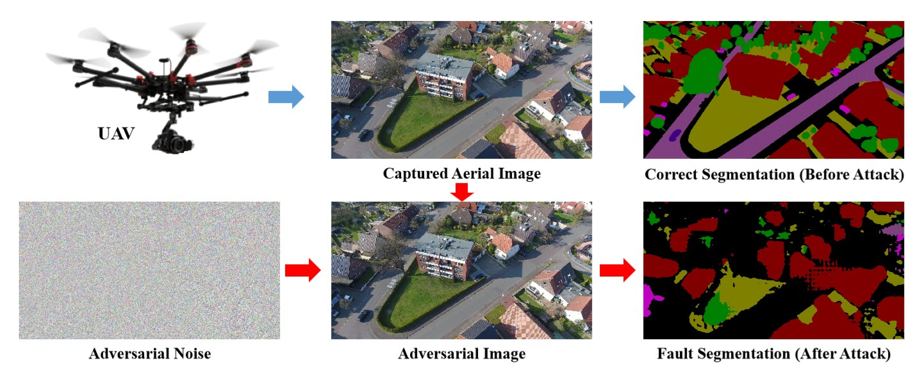
For the geoscience and remote sensing community, studies on adversarial examples have also received attention. Czaja et al. [31] first analyzed the influence of adversarial patches on satellite remote sensing image classification. Li et al. [32] constructed a remote sensing image classification model against white-box adversarial attack. Chen et al. [33] analyzed the negative impact of adversarial examples on remote sensing scene interpretation. Li et al. [34] demonstrated that adversarial examples would destroy the performance of CNN-based SAR image classifiers. In [35], Xu et al. designed a robust hyperspectral image classification network against adversarial attacks. Chen et al. [36] assess the influence of black-box and white-box adversarial attacks on remote sensing scene classification. Xu et al. [37] proposed an adversarial training strategy to improve the robustness of the remote sensing image classification model to adversarial examples. In [38], Cheng et al. designed a universal adversarial example attack strategy for remote sensing image classification. However, these studies focus on the problem of adversarial attacks in aerial image classification tasks, ignoring the impact of adversarial attacks on aerial image semantic segmentation. Moreover, existing studies commonly use adversarial training or adversarial sample detection methods to resist the interference of adversarial noise without considering the contribution of global features in defending against adversarial example attacks. In Figure 1, we illustrate the adversarial attacks for aerial image semantic segmentation. As shown in Figure 1, the CNNs model can obtain accurate semantic segmentation results for the original image while adding adversarial noise seriously affects the segmentation effect.
Existing studies [35,39] have demonstrated that global features have better robustness against adversarial attacks. To defend against adversarial example attacks faced by aerial image semantic segmentation, in this article, we propose a robust aerial image semantic segmentation method, namely the global feature attention network (GFANet). Based on the robust characteristics of global features, we design the global context encoder (GCE), global coordinate attention mechanism (GCAM), and feature consistency alignment (FCA) for mining the global feature information contained in aerial images. In addition, we construct a universal adversarial training strategy to enhance the robustness of the model against adversarial attacks. The contributions of this study are summarized as follows.
  • We systematically analyze the impact of adversarial attacks on aerial image semantic segmentation for the first time and propose a robust aerial image semantic segmentation network based on global context feature information awareness and fusion.
  • We construct the global context encoder (GCE) module, global coordinate attention mechanism (GCAM), and feature consistency alignment (FCA) module to resist adversarial noise interference by using the robust characteristics of global features.
  • We design a universal adversarial training strategy to enhance the defense of the semantic segmentation model against different adversarial example attacks by introducing Gaussian noise in the adversarial training process.
  • The extensive experiments conducted on three aerial image datasets containing large-scale urban and suburban scenes demonstrate the robustness of the proposed method against adversarial attacks while maintaining high semantic segmentation accuracy.

2. Related Works

In this section, we review the existing global feature extraction, adversarial attacks, and adversarial defense methods.

2.1. Global Feature Extraction

The extraction of global feature information is essential for various computer vision tasks. It can improve the performance of the CNN model and make it robust against adversarial attacks [39]. However, global feature extraction is challenging for CNN-based models because it needs to consider both local and long-range dependencies. For semantic segmentation tasks, extracting global feature information from images has received extensive attention. Zhang et al. [40] constructed the context encoding module to encode the semantic information and obtain global details by using the relative position relationship of pixels. PANet [41] introduces the global attention unsample module in each encoder layer to model global context information to obtain long-range spatial dependencies. CGNet [42] uses the context-guided module to encode local pixel regions and then uses the feature correlation of local pixels to obtain global context information. HRCNet [43] constructs the context feature interaction structure to splice local features, and the semantic inference module is used to fuse local and global features. Nekrasov et al. [44] designed the global deconvolution model to enhance the resolution of context features and used the spatial interaction to model local spatial dependencies. Zhang et al. [45] designed the context feature aggregation module to obtain global feature information by context aggregation of different scale features. Li et al. [46] construct the hybrid attention module to enhance the edge distribution of the ground object and use the non-local attention mechanism to model the global context information. SPANet [47] uses synergistic attention to obtain spatial and channel features and uses a hierarchical embedded-synergistic attention perception module to aggregate global context information. CANet [48] constructs the covariance attention to model the global feature information and establishes the context dependency by obtaining the relationship between local pixels. In this article, inspired by [40,42,45,48], we construct GFANet based on the robust characteristics of global features, which can obtain better semantic segmentation accuracy and be robust to adversarial example attacks.

2.2. Adversarial Attacks

The adversarial example belongs to the evasion attack in image classification tasks [23]. The attacker constructs adversarial noise with weak perturbation based on the differentiable loss function to destroy the classifier performance.
max L ( x + η , y , θ ) , s . t . η p ε
where, x is the clean image sample, y is the category label corresponding to the input image, θ denotes the model parameter variable, η denotes the adversarial perturbation, L · is the classifier loss function, and · p denotes the p norm. The optimization objective of Equation (1) is to obtain the optimal adversarial perturbation η under the restriction of perturbation amplitude ε to maximize the classifier loss.
(1) Fast Gradient Sign Method (FGSM): In fact, FGSM can be interpreted as a gradient ascent method [24]. In the linear model, the perturbation variables that FGSM expects to add are consistent with the gradient direction of the model loss function, and its formal description is as follows.
x ^ = x + α sign x L x , y , θ
where α is the hyper-parameter used to adjust the perturbation amplitude, sign · is the sign function, and x L · is the gradient of the loss function L · to the input image x.
(2) DeepFool: The DeepFool attack [25] assumes the classifier model is linear, and each category has a decision boundary (i.e., decision hyperplane). DeepFool solves the optimization problem of Equation (3) using multiple iterations to obtain perturbations that satisfy the f ( x ^ ) f ( x ) .
x ^ k + 1 = x ^ k f x ^ k x L f x ^ k , t 2 2 x L f x ^ k , t
where f x denotes the predicted label of the input image, t denotes the target category in the attack, and compared with FGSM [24], the DeepFool generates less perturbation.
(3) Jacobian-Based Saliency Map Attack (JSMA): Compared with other attack methods, JSMA [26] introduces the concept of the saliency map, which obtains the best attack effect by modifying the minimum pixel of clean samples. JSMA uses 0 norm to constrain the generation of adversarial perturbation, and its optimization objective is as follows.
Δ r = min r r 0 , s . t . f x + r f x
where Δ r represents the optimal perturbation of the adversarial examples, r represents the initial perturbation variable, and · 0 represents the 0 norm constraint.
(4) Carlini–Wagner (C&W): The C&W attack [27] includes three attack modes under 0 , 2 , and norm constraints, which mainly attack a distillation network with strong defense capability. C&W generate adversarial perturbations by solving a norm-restricted constrained optimization problem.
min r p + c · f x + r , s . t . x + r 0 , 1 n
where · p represents the norm constraint. By optimizing Equation (5), C&W can improve the confidence of misclassification labels under the condition of small perturbation value.
(5) Projected Gradient Descent (PGD): The PGD attack [28] can be regarded as the iterative version of FGSM [24]. The basic idea is to use x ^ 0 = x + r a m d o m ε , ε as the initialization value and calculate the gradient of x ^ by iterations to update the adversarial examples.
x i + 1 = clip x , ε x i + μ sign x i L x i , t
where μ represents the iterative step and clip · represents for constraining within the ε -neighbor ball of input image x.
(6) Universal Adversarial Perturbation (UAP): The UAP attack [30] can generate the adversarial perturbations without any image samples. The generated adversarial examples are universal because perturbation r satisfies the following constraints.
P f x + r f r 1 δ , s . t . r p ε
where · p represents the p norm constraint, r represents the perturbation variable, δ is the desired fooling rate, and ε is used to limit the amplitude of adversarial perturbation.

2.3. Adversarial Defense

To resist adversarial attacks, many defense methods have been proposed, including adversarial training, adversarial example detection, and modified network architecture.
(1) Adversarial Training: The adversarial training strategy is to introduce adversarial examples in the process of model parameter optimization to improve the robustness against adversarial attacks [28]. The process of adversarial training is equivalent to solving the following maximin problem.
min f E max x ^ B ( x , ε ) L f ( x ^ ) , y
where x represents clean examples, x ^ represents adversarial examples, y represents the corresponding true labels, and L · represents the loss function. B ( x , ε ) is the space with x ± ε as the upper and lower bounds. In the process of solving the internal maximization of max L f ( x ^ ) , y , the PGD attack [28] is used to generate adversarial examples to approximate the solution, while for the external minimization problem of min E · is to minimize the adversarial loss caused by the internal adversarial examples by updating the model parameters. Zhang et al. [49] modified the adversarial training, transforming the training process into the approximate solution to the following maximin problem.
min f E L f ( x ) , y + α · max x ^ B ( x , ε ) L f ( x ^ ) , f
where α represents the regular term. This method balances the accuracy of clean examples and adversarial examples and obtains better adversarial defense effects. Liu et al. [50] trained the deep neural network by adding Gaussian noise to the image for data enhancement to reduce the model sensitivity to adversarial noise. Wang et al. [51] constructed the misclassification-aware adversarial training strategy, which trains the robust model by distinguishing the incorrectly and correctly classified samples in the training process.
(2) Adversarial Example Detection: In addition to adversarial training, another approach to address adversarial attacks is adversarial example detection. The existing adversarial example detection methods include metric-based methods and prediction inconsistency-based methods. For metric-based methods, Feinman et al. [52] used kernel density estimation and Bayesian uncertainty to discriminate the adversarial subspace to separate clean adversarial examples. Ma et al. [53] proposed a detection method based on local intrinsic dimension measurement, which constructed the separation hyperplane of clean and adversarial examples by estimating intrinsic dimension to achieve adversarial example detection. Grosse et al. [54] uses an addition outlier class C o u t to strengthen the model training process. In the test stage, the trained model can classify the adversarial examples into the C o u t class. Since adversarial examples are inconsistent with clean examples, adversarial examples detection can be achieved by comparing their differences. Tao et al. [55] detect adversarial examples by measuring the inconsistency between the clean example and adversarial example training models. Feinman et al. [56] used dropout technology to generate multiple classifier models to detect adversarial examples by identifying inconsistencies in the output of different classifiers. Xu et al. [57] limited the available subspace of adversarial examples by using the feature compression squeezing technique and then set a fixed threshold to detect adversarial examples.
(3) Modified Network Architecture: Modifying the model architecture and parameters is another effective to against adversarial attacks. Inspired by the denoising autoencoders, Gu et al. [58] constructed the deep compression network to suppress the adversarial noise interference. Ross et al. [59] use gradient regularization to improve the model’s robustness against adversarial attacks. Hinton et al. [60] use knowledge distillation to transfer teacher network parameters to student networks and use feature compression against adversarial attacks. Nayebi et al. [61] introduce the enhanced nonlinear activation function to improve the model nonlinear learning against adversarial examples. Cisse et al. [62] uses the global Lopschitz constant to control the gradient optimization direction and uses the gate optimization coefficient to enhance the model robustness. Gao et al. [63] design the DeepCloak framework, which introduces the nonlinear units in the classification layer to suppress adversarial noise interference. Sun et al. [64] construct robust deep neural networks against adversarial example attacks based on statistical filters.

3. Methodology

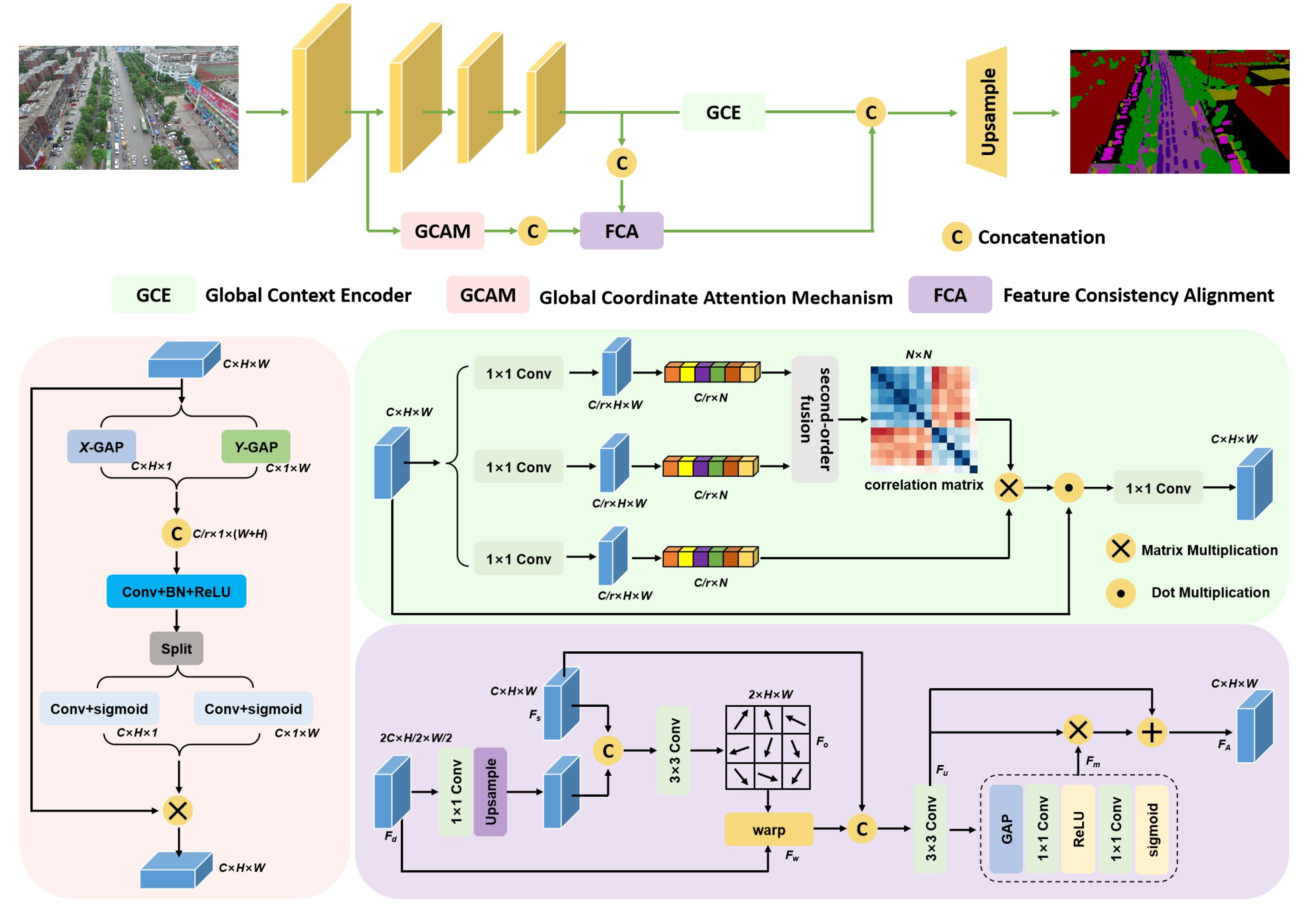
The overall architecture of GFANet is shown in Figure 2, which includes the backbone network, global context encoder (GCE) module, global coordinate attention mechanism (GCAM), and feature consistency alignment (FCA) module. Specifically, we use VGG16 [65] as the backbone network to extract primary feature information. Then, the GCE module performs a global context encoder on the primary features to obtain the long-range spatial dependency. To further mine global feature information and suppress adversarial noise interference, GCAM and FCA module are used to enhance the global representation of deep and shallow features and achieve multi-scale feature fusion.

3.1. Global Context Encoder

Extracting the global context of high-dimensional features can obtain global dependencies between features, effectively reduce the impact of adversarial noise, and enhance the robustness against adversarial attacks. Inspired by previous work in [35], we propose a global context encoder module, which re-adjusts the dependence of different feature spatial positions by second-order linear fusion of high-dimensional features to obtain the spatial position correlation matrices. Compared with the reshape and transpose operation in the existing attention mechanism, the second-order linear fusion can perform bilinear fusion on different features in spatial positions and reduces feature information loss. As shown in Figure 2, the global context encoder module uses feature map F R C × H × W as input, and uses two 1 × 1 convolutions to reduce the dimension of feature F to obtain feature maps F 1 R C / r × H × W and F 2 R C / r × H × W , where r represents the dimension reduction coefficient. To obtain the global representation, the features F 1 and F 2 are stretched in the spatial dimension to obtain the spatial vectors V 1 R C / r × H × W and V 2 R C / r × H × W . To realize spatial vector fusion, we use bilinear pooling [66] to fuse spatial vectors V 1 and V 2 to obtain spatial fusion matrix. The obtained spatial fusion matrix contains a global representation between the pixel positions of different features. To enhance the nonlinear representation, we use the Softmax function to normalize the spatial fusion matrix in spatial position, and the calculation is as follows.
S j i = exp V 1 i · V 2 j i N exp V 1 i · V 2 j
where S j i represents the encoder of the ith position on the spatial pixel to the jth position, and V i j represents the jth element of the feature vector V i .
To further enhance the feature global representation, we perform the same operation for feature F as V 1 and V 2 to obtain the spatial vector V 3 and residual connection with the feature F to obtain the global context feature E , and the specific calculation is as follows.
E j = j = 1 C / r i = 1 N V 3 i · S j i + F j
where N represents the dimension of spatial fusion matrix S j i , and C / r represents the channel dimension of feature map. To restore the channel dimension of the feature map, we use 1 × 1 convolution to map the feature E to the original feature channel dimension.

3.2. Global Coordinate Attention Mechanism

To further enhance the global feature representation and suppress the adversarial noise interference, inspired by previous work in [67,68], we construct a global coordinate attention mechanism. Different from the existing coordinate attention mechanism [69], the global coordinate attention mechanism performs a spatial two-dimensional encoder on the input features and performs feature aggregation along two spatial directions, one of which can obtain long-range dependency, and the other can obtain spatial position information. The generated feature map is encoded into a pair of direction-aware and position-sensitive attention feature maps, which are complementary to the input features to achieve global feature enhancement. As shown in Figure 2, for the input feature x R C × H × W , the global coordinate attention mechanism performs global average pooling (GAP) on the W and H directions to obtain feature maps z h R C × H × 1 and z w R C × 1 × W .
z h = 1 W 0 i < W x h , i
z w = 1 H 0 j < H x j , w
where W and H represent the width and height of feature map x . For feature z h and z w , we fuse features on the spatial dimension and then use convolution and the nonlinear activation function to obtain the fusion feature f R C / r × 1 × H + W , where the convolution operation compresses the channel dimension to C / r using the channel scaling factor r.
f = δ F z h , z w
where, · , · represents the feature splicing operation, F represents the convolution operation, and δ represents the nonlinear activation function. Then feature f is decomposed into independent tensors f h R C / r × H × 1 and f w R C / r × 1 × W on the spatial dimension, and convolution and activation operations are performed on f h and f w to obtain attention feature vectors g h R C × H × 1 and g w R C × 1 × W .
g h = δ F h f h
g w = δ F w f w
where F h and F w represent convolution operations in different directions. The attention feature vectors are fused with the original feature to obtain the global enhanced feature y R C × H × W . The calculation is as follows.
y i , j = x i , j × g h i × g w j
where the broadcast mechanism is used to superimpose the W direction feature g w j and the H direction feature g h i on the feature x , and the global enhancement feature y i , j is consistent with the size of the original feature x i , j .

3.3. Feature Consistency Alignment

For aerial image semantic segmentation, shallow convolution contains high-resolution spatial structure features, and deep convolution contains low-resolution local detail features. Previous studies [10,11,12] use bilinear interpolation to upsample low-resolution features and then fuse them with high-resolution features. However, due to the influence of adversarial noise, the use of bilinear interpolation will expand the interference of adversarial noise. As shown in Figure 2, the constructed feature consistency alignment module takes the deep feature F d R H / 2 × W / 2 × 2 C generated by the global coordinate attention mechanism and the shallow feature F s R H × W × C obtained by the backbone network as input features. The 1 × 1 convolution is used to reduce the channel dimension of deep feature F d and upsample to the size consistent with F s . Then, the channel fusion is carried out between the upsampling feature and F s , and the 3 × 3 convolution is used to obtain the two-dimensional offset F o R H × W × 2 . Each pixel position of the offset contains horizontal and vertical offsets. Based on the two-dimensional offset F o , the spatial transformation function w a r p is performed on the deep feature F d to obtain the feature F w , and splice it with shallow feature F s . To obtain the global information of channels, the 3 × 3 convolution is used on the spliced features to obtain feature F u , then the global average pooling is used to obtain the global information of each channel, and the 1 × 1 convolution is used to increase the linear correlation of channel information. Finally, the sigmoid function is used to establish the channel correlation weight parameter F m and act on F u to obtain the consistent alignment feature F A . The calculation process of feature consistency alignment is as follows.
F o = f 3 × 3 c o n c a t F s , u p s a m p l e f 1 × 1 F d
where F o represents the two-dimensional offset, and f 1 × 1 and f 3 × 3 represents 1 × 1 and 3 × 3 convolution operations. Based on the offset F o , the deep feature F d is spatially transformed to obtain the feature F w .
F w = w a r p F h , F o
where w a r p · represents the spatial transformation function. The spatial transformation feature F w is spliced with the shallow feature F s , and the splicing feature F u is obtained by using 3 × 3 convolution.
F u = f 3 × 3 c o n c a t F w , F s
where c o n c a t · represents the splicing function. The global average pooling is used to obtain the global channel feature of the splicing feature F u , and then the channel dimension is adjusted by 1 × 1 convolution, and the sigmoid function is used to obtain the global channel feature F m . The global channel feature F m and the splicing feature F u are fused to obtain the global consistency feature F A .
F m = s i g m o i d f 1 × 1 ReLU f 1 × 1 G A P F u
F A = F u F m F u
where ReLU · represents the activation function, G A P · represents the global average pooling, F m represent the global channel feature, F A represent the global consistency fusion feature, ⊕ represents the matrix addition, and ⊗ represents the matrix multiplication.

3.4. Universal Adversarial Training

As an effective means against adversarial example attacks, adversarial training [28] can effectively improve the model’s robustness against adversarial noise. The principle of adversarial training is to solve the maximin optimization problem. The formal description is as follows,
min θ max x a d v : x a d v x ε L h θ x a d v , y t r u e
where x a d v represents the adversarial example, x represents the clean example, ε represents the adversarial perturbations, L · represents the loss function, h · represents the training model with parameter θ , and y t r u e represents the ground truth corresponding clean examples. For our semantic segmentation model, cross-entropy is used as a semantic segmentation loss function. The cross-entropy loss is calculated as follows.
L = c = 1 M y c log p c
where M represents the number of object categories, y c represents the indicator variable (0 or 1), and p c represents the probability that the predicted result belongs to the c t h category.
The adversarial training process adds adversarial perturbation ε to the clean examples to approximate the internal maximin of the loss function and then optimize the model parameter θ . Inspired by previous work in [28,50], we proposed a universal adversarial training strategy, which uses StepLL attack [29] to generate adversarial examples for adversarial training and introduces Gaussian perturbations in the process of adversarial training to improve the robustness of the model against different adversarial example attacks. The proposed universal adversarial training process is shown in Algorithm 1, where N μ , σ 2 is the Gaussian distribution with mean μ and variance σ 2 .
Algorithm 1: Universarial Adversarial Training.
Input: adversarial training times T, iteration times I, training set label number M, training set x i , y i t r u e , target label y i t a r g e t , perturbation ε , iteration perturbation stride α , mean μ , variance σ 2 .
Output: model parameter θ .
 1: for t 1 to T do
 2:   for i 1 to M do
 3:      x i a d v = x i + max min N μ , σ 2 / 255 , ε , ε
 4:     for  j 1 to I do
 5:       x i a d v = x i a d v α · f x i a d v
 6:       f x i a d v = sign x i a d v L h θ x i a d v , y i t a r g e t
 7:       x i a d v = max min x i a d v , x i + ε , x i ε
 8:    end for
 9:     θ = θ θ L h θ x i a d v , y i t r u e
 10:   end for
 11: end for

4. Experiments and Analysis

4.1. Dataset Information

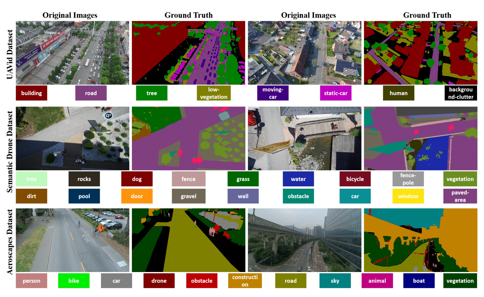
To verify the effectiveness and feasibility of the proposed method, we conducted experiments on three UAV aerial image benchmark datasets, including the UAVid dataset [2], Semantic Drone dataset [70], and Aeroscapes dataset [71].
The details of these datasets are as follows.
UAVid is a challenging benchmark dataset for UAV aerial image semantic segmentation, which contains many static and moving objects in complex urban scenes. This dataset is captured using the resolution video recording mode, and the image sizes are 3840 × 2160 pixels. Since UAVid is mainly collected from urban scenes, the dataset contains eight object classes in urban scenes, namely building, road, tree, low-vegetation, moving-car, static-car, background-clutter, and human. There are 420 images in the dataset, of which we use 200 images for training, 70 images for validation, and the remaining 150 images for testing. Due to the large size of the original image, the image size is scaled to 1024 × 1024 pixels. The sample image and corresponding labels are shown in Figure 3.
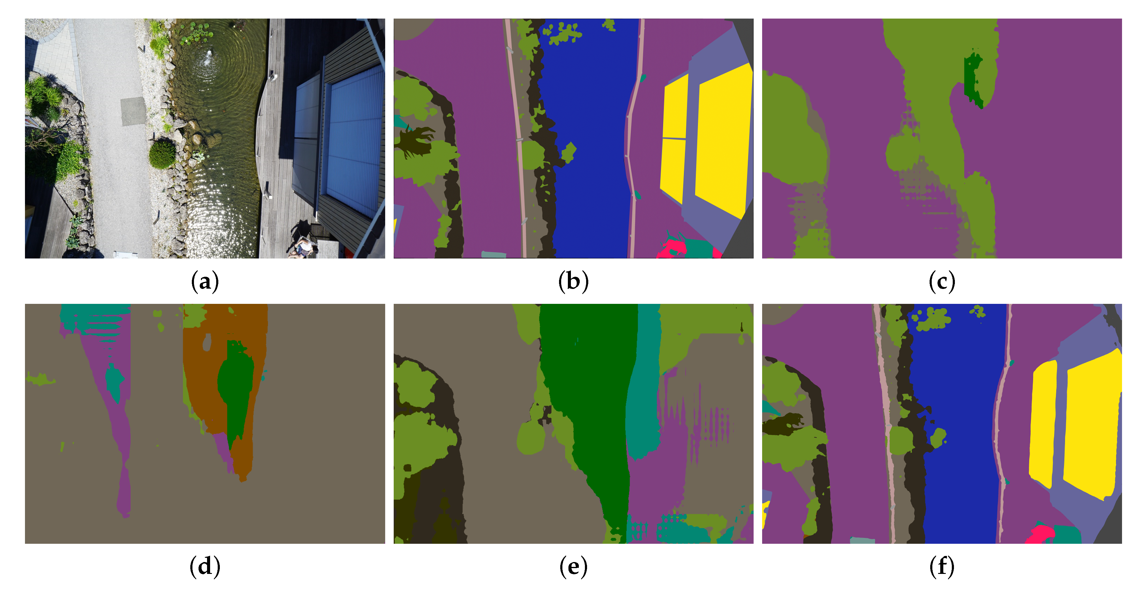
Semantic Drone focuses on semantic understanding of urban scenes; this dataset observes ground objects from the bird’s eye perspective at an altitude of 5 to 30 m. The high-resolution camera is used to capture images at a size of 6000 × 4000 pixels, and the dataset contains eighteen classes of ground objects, such as trees, rocks, dogs, fences, grass, water, bicycle, fence-pole, vegetation, dirt, pool, door, gravel, wall, obstacle, car, window, and paved-area. The original image and label are shown in Figure 3. This dataset contains 400 publicly available images; 280 images in the dataset are used as the training set, 40 images as the validation set, and 80 images as the testing set. To facilitate training, we crop the original image size from 6000 × 4000 pixels to 2048 × 1024 pixels.
AeroScapes dataset is more challenging for semantic segmentation tasks because it includes the ground objects in complex urban and suburban scenes. The AeroScapes dataset contains 3269 images and eleven categories of ground objects, namely person, bike, car, drone, boat, animal, obstacle, construction, vegetation, road, and sky. As shown in Figure 3, the number of pixels for different object categories in the dataset varies greatly. The image size in the dataset is 1280 × 720 pixels, and we maintain the original image size constant during the training process. For the 3269 images contained in the dataset, we use 2288 images as the training set, 654 images as the validation set, and the remaining 327 images for testing.

4.2. Experimental Setup and Implementation Details

To verify the robustness of the proposed method against adversarial example attacks, we use FGSM [24], C&W [27], and PGD [28] attack methods to construct corresponding adversarial example test sets. Specifically, for UAVid [2] dataset, we use FGSM to construct adversarial examples, and for Semantic Drone [70], and AeroScapes [71] datasets, we use C&W and PGD attacks. We adopt the FGSM with norm to conduct untargeted adversarial attacks using Equation (2), where the ε is fixed to 0.04. For C&W attack, we use the 0 norm to conduct un-targetted adversarial attacks using Equation (5), the number of iterations T is fixed to 10, and the parameter c is set to 0.1. Equation (6) generates PGD adversarial examples, where the perturbation constraint ε is set to 0.01, iteration stride μ is set to 2, and iteration number T is fixed to 20.
To ensure the credibility of the experimental results, we randomly selected images in the dataset to form the training set, validation set, and testing set and repeated the experimental process 10 times. In addition, we use data augmentation methods such as random inversion, size cropping, and brightness transformation to increase the number of dataset samples. We implement the Pytorch platform to build the proposed semantic segmentation network, and the experiments are carried out with an Intel i9-12900T CPU with 64 GB RAM, NVIDIA GTX GeForce 3090 GPU, and Ubuntu 18.04 operating system. The training epochs are set as 1000, and the batch size is set to 8. For model training optimization, set the initial learning rate to 0.001, and SGD is used with a momentum of 0.9 as the optimizer. In addition, we give detailed steps to perform adversarial attacks against the proposed GFANet, as shown in Algorithm 2. The goal of adversarial attacks on aerial image semantic segmentation tasks is to use adversarial noise to interfere with the original image to maximize the number of misclassification of all test pixels in the image.
Algorithm 2: Adversarial Attack on GFANet.
Input:
 1: Aerial image x and corresponding ground truth y.
 2: Semantic segmentation model f with parameters θ .
 3: Adversarial perturbation amplitude ε , training epochs τ , and learning rate η .
Output: The predictions on the adversarial example x a d v .
 4: Initialize model parameters θ with uniform distribution.
 5: for t in r a n g e 0 , τ  do
 6:    Compute the global context features E via (11).
 7:    Compute the coordinate attention features Y via (17).
 8:    Computer the global consistency features F via (22).
 9:    Computer the cross-entropy loss L via (24).
 10:    Update θ by descending its stochastic gradients.
 11: end for
 12: Generate the adversarial image x a d v via (2), (4), (5).
 13: Feed the adversarial image x a d v to the trained model f to achieve the segmentation.

4.3. Evaluate Metrics

To compare the performance of the semantic segmentation network, we adopt the PA, mPA, F1_score, and mIoU as evaluation metrics. First, we define t p , f p , f n , and t n as true positives, false positives, false negatives, and true negatives.
  • The PA is the basic evaluate metric in semantic segmentation, which is defined as the correctly classified pixel in all pixels as P A = t p + t n / t p + t n + f t + f n .
  • The mPA is the mean of the sum of category pixel accuracy (cPA), where c P A = t p / t p + f p represents the correct proportion of predicted category i t h pixels.
  • The F1_score is the geometric mean between the precision (P) and recall (R) of each class as F 1 _ s c o r e = 2 × P × R P + R , where P = t p / t p + f p and R = t p / t p + f n .
  • The mIoU is defined as the mean of IoU, and the IoU is calculated as I o U = P i G i / P i G i . P i and G i are the set of prediction pixels and ground truth pixels for the ith class.

4.4. Comparison with State-of-the-Art Methods

For experimental comparison, we verify the model semantic segmentation performance and the robustness against adversarial attacks. On the UAVid dataset, we compare the GFANet with the existing aerial image semantic segmentation networks LANet [10], AERFC [11], and AFNet [12]. For the Semantic Drone, we compare the proposed method with the MCLNet [13], BSNet [14], and SBANet [15]. For the AeroScapes dataset, the GFANet is compared with MANet [16], HPSNet [17], and TCHNet [72].
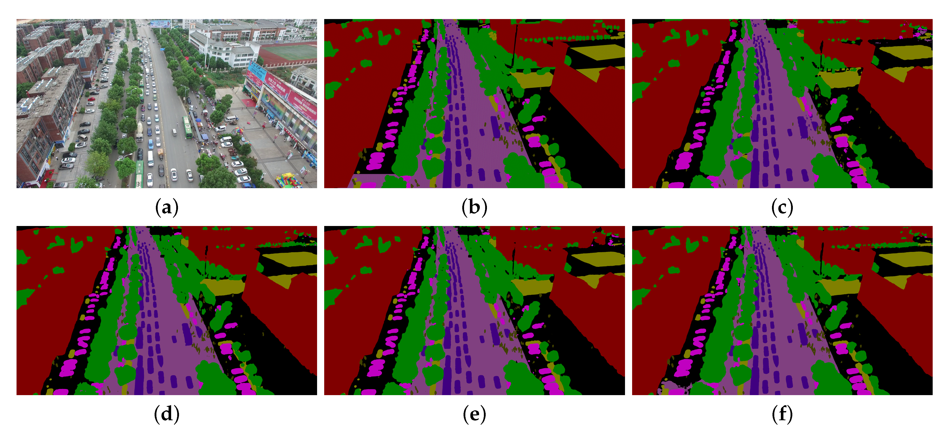
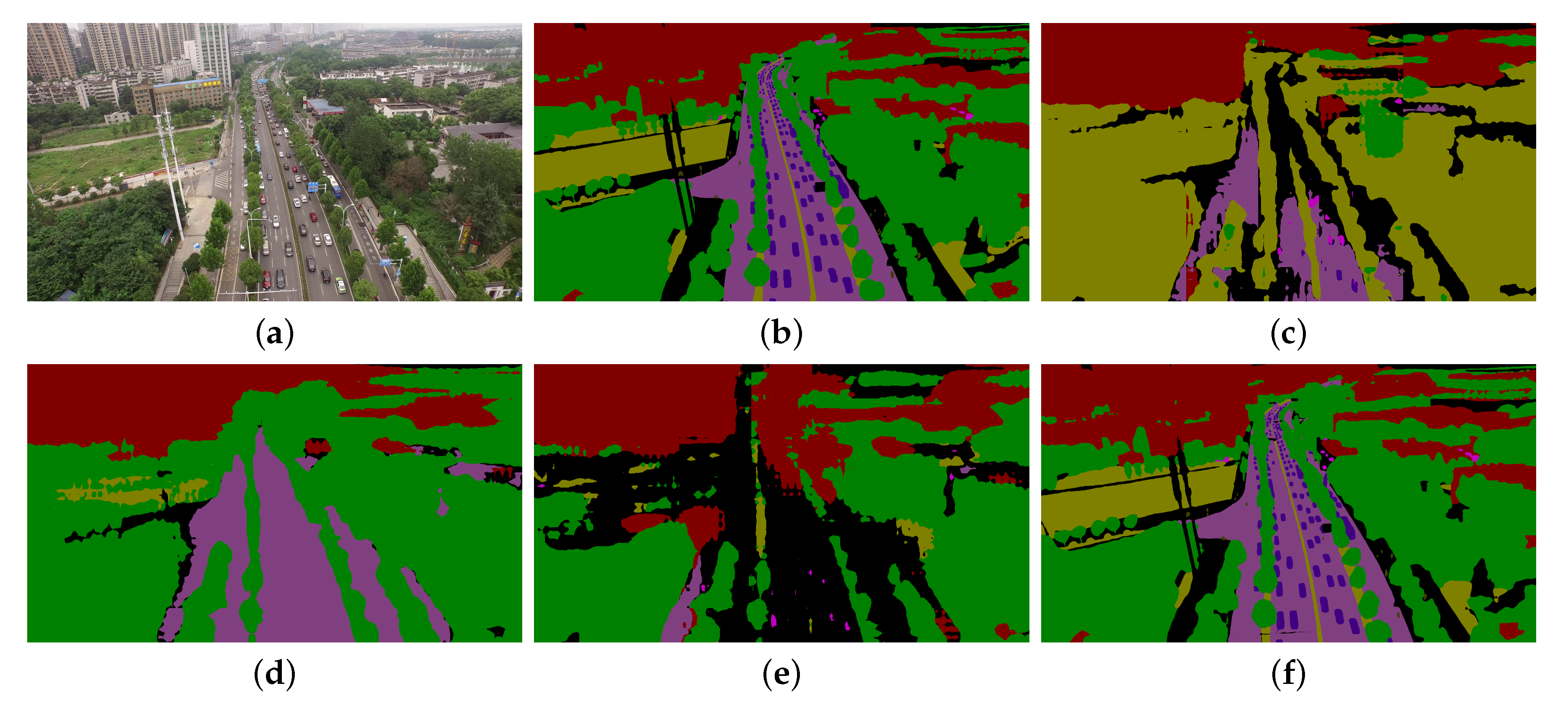
Compare on UAVid Dataset: First, we compared performance on the clean example test set, and the quantitative results and visual comparisons are shown in Table 1 and Figure 4. Second, the robustness against adversarial attacks is verified on the adversarial example test set generated by FGSM attack [24], and the results are shown in Table 2 and Figure 5. Next, we give the performance analysis and robustness against attacks of different methods.
(1) LANet [10]: This network consists of a patch attention mechanism and attention embedding module, which can mine local feature information of the ground objects to guide the model to complete semantic segmentation. As shown in Table 1, LANet achieves 66.52% mIoU on the clean example test set, while only 15.85% mIoU is completed on the adversarial example test set. The visualization results in Figure 4 and Figure 5 show that LANet can better predict the pixels of each category for clean examples, which for adversarial samples, there are serious mistakes, such as the “tree” is misclassified as “low-vegetation”. The results in Figure 6 further shows the performance difference between LANet for clean and adversarial examples, with the mIoU decreasing by 50.67%. The experimental results also further demonstrate the poor performance of local features against adversarial attacks.
(2) AERFC [11]: To achieve accurate segmentation of different scale objects, AERFC constructs the adaptive convolution kernel to extract multi-scale feature information of ground objects. The results in Table 1 show that AERFC has a better semantic segmentation effect on different categories of objects; for example, its mPA and mIoU reach 79.85% and 69.28%, respectively. For adversarial examples, the results in Table 2 show that the mPA and mIoU of AERFC only reach 18.23% and 15.46%. The visualization results in Figure 4 and Figure 5 further show the performance difference of AERFC on clean examples and adversarial examples. For example, for the clean sample test set, AERFC achieves better prediction for different categories of object pixels, while its performance on the adversarial sample test set is significantly degraded. The experimental results of AERFC show that multi-scale features cannot be against the impact of adversarial attacks.
(3) AFNet [12]: For the purpose of feature enhancement, AFNet constructs the scale-feature attention mechanism and scale-layer attention module, which achieves semantic segmentation by enhancing features of different scales and different convolution layers. From Table 1, we can observe that AFNet has better semantic segmentation performance on the clean sample test set, while the results of Table 2 show that AFNet performs poorly on the adversarial sample test set. The visualization results also show the performance difference of AFNet on clean samples and adversarial samples. For example, in Figure 4, AFNet can accurately predict the object “road”, while for adversarial examples, “road” is misclassified as “background-clutter”. It can be seen from Figure 6 that the mIoU of AFNet decreased from 70.47% of clean samples to 19.75% of adversarial samples. The experimental results of AFNet show that simple feature enhancement cannot alleviate the impact of adversarial samples on model performance.
For our proposed GFANet, it can be seen from Table 1 and Table 2 that GFANet achieves the best results on both clean and adversarial sample test sets. For clean samples, the mIoU reaches 71.89%, while for adversarial samples, its mIoU reaches 69.51%. The visualization results of Figure 4 and Figure 5 also prove that GFANet can complete accurate semantic segmentation for clean and adversarial samples. From Figure 6, it can be observed that the mIoU difference between GFANet for clean and adversarial samples is only 2.38%, which further indicates the robustness of GFANet against adversarial example attacks. The experimental results of GFANet show that the global features can complete accurate aerial image semantic segmentation tasks and have strong robustness against adversarial attacks.
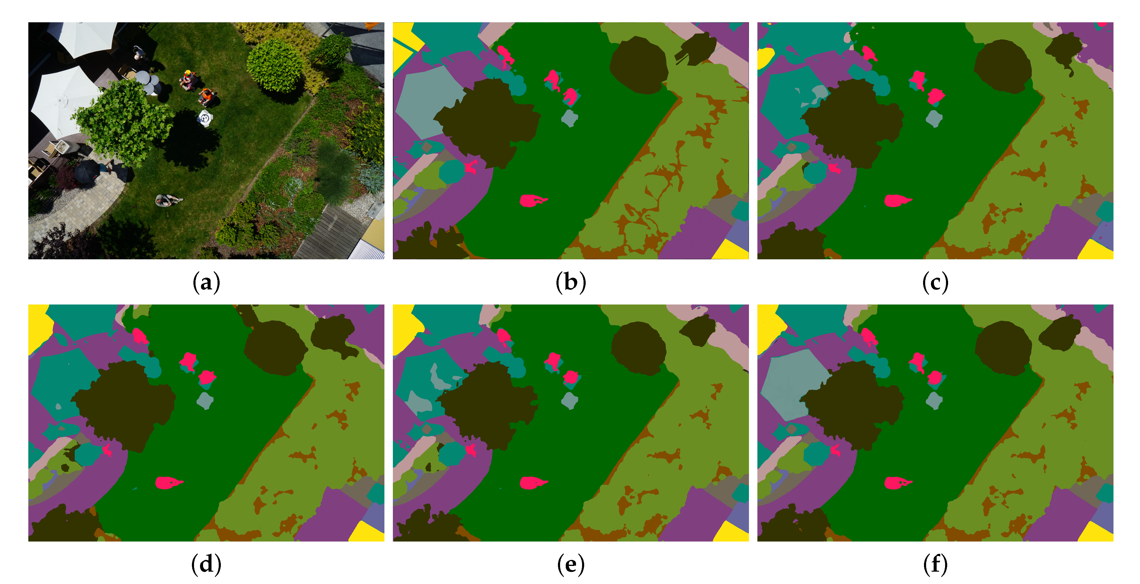
Compare on Semantic Drone Dataset: Since the dataset contains more object categories and complex scenes, it can further verify the semantic segmentation accuracy and the robustness against adversarial attacks of different methods. We use C&W attack [27] with l 0 norm to generate an adversarial example test set. Table 3 and Figure 7 show the experimental results of different methods on the clean sample test set, and Table 4 and Figure 8 show the results on the adversarial example test set. Next, we analyze the experimental results of different methods in detail.
(1) MCLNet [13]: To enhance the correlation between multi-scale features, MCLNet constructs the multi-scale calibration learning strategy. The network performs semantic segmentation by mining the correlation between local and global features. The experimental results on the clean sample test set in Table 3 and Figure 7 show that MCLNet can better segment objects of different scales, and its mAP and mIoU reach 73.81% and 62.52%. However, for the adversarial example test set, as shown in Table 4, the performance of MCLNet is significantly degraded, with mAP and mIoU 23.16% and 12.85%. From the visualization results of Figure 8, it can be seen that the adversarial attack has a great impact on the performance of MCLNet, and it cannot complete accurate semantic segmentation on the adversarial sample test set. It can also be observed from Figure 6 that the adversarial example attack reduces the mIoU of MCLNet by 39.36%. The experimental results further illustrate that only establishing the correlation between local and global features is ineffective against adversarial example attacks.
(2) BSNet [14]: This network consists of dynamic hybrid gradient convolution and coordinates sensitive attention, which completes semantic segmentation by obtaining the salient boundary information of the object region. As shown in Table 3, the mPA and mIoU of BSNet are 74.29% and 65.13%, which shows the contribution of boundary feature information in accurate semantic segmentation. From the visualization results of Figure 7, it can be seen that BSNet can finely segment the contour boundary. For the adversarial example test set, as shown in Table 4, the mIoU of BSNet on the adversarial example test set is only 26.35% and 15.07%, which is obviously inferior to the experimental results on the clean example test set. From Figure 6, it can be seen that the mIoU of BSNet decreased from 65.13% to 15.07%. The results of Figure 8 further prove the impact of adversarial examples on the performance of BSNet, which cannot complete the semantic segmentation task under adversarial example attacks. The results of BSNet also show that only enhancing boundary features cannot alleviate the impact of adversarial examples on model performance.
(3) SBANet [15]: To obtain the fine-grained semantic features of the object region, SBANet uses the boundary attention mechanism to locate the object region and uses the adaptive weighted multi-task learning guidance model to complete the semantic feature extraction. As shown in the clean example experiment results in Table 4 and Figure 7, SABNet obtained 76.82% and 68.07% of mAP and mIoU and completed accurate semantic segmentation for different object categories. However, the experimental results of Table 4 and Figure 8 show that SBANet is ineffective against adversarial example attacks. The mIoU of SBANet on the adversarial example test set is only 16.72%, and there are pixel classification errors, such as the “water” is misclassified as “vegetation”. The results in Figure 6 show that the adversarial examples reduce the mIoU from 68.07% to 16.72%. The experimental results of SBANet verify that semantic features are ineffective against adversarial attacks.
As shown in Table 3 and Table 4, GFANet achieves the mIoU of 74.80% and 73.20% on clean example and adversarial example test sets, which is superior to other compared methods. The visualization results of Figure 7 and Figure 8 show that GFANet can complete accurate semantic segmentation and effectively alleviate the impact of adversarial example attacks.
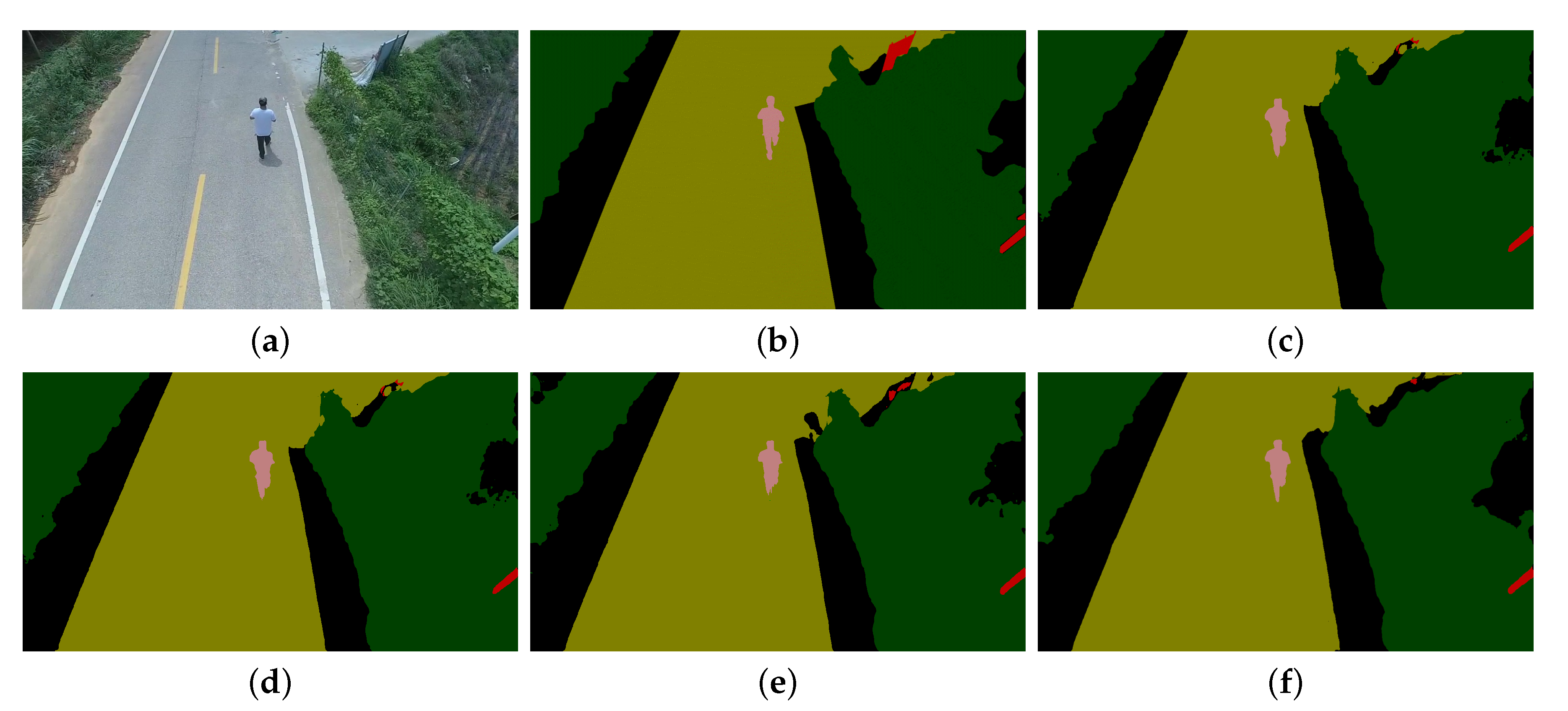
Compare on Aeroscapes Dataset: The dataset contains many suburban scenes and has higher resolution and fine annotation information, which can effectively verify the robustness and generalization ability of the semantic segmentation network. For the adversarial example attack, we use the PGD attack [28] to generate the adversarial example test set. Figure 9 and Figure 10 show the visual comparison results. The specific performance analysis of different methods is as follows. Correspondingly, Table 5 and Table 6 show the quantitative comparison results of different methods on clean example and adversarial example test sets.
(1) MANet [16]: This network uses a multi-attention cascade to obtain multi-scale context features and uses dot-product attention for feature fusion. MANet effectively alleviates the feature loss problem in the feature fusion process. As shown in Figure 9 and Table 5, for the clean example test set, MANet obtains complete object region contour information and achieves accurate pixel classification for different category objects, with mPA and mIoU of 81.36% and 69.89%. However, for the adversarial example test set, the quantitative comparison results in Table 6 show that the mIoU of MANet only reaches 9.95%. From Figure 9, it can be observed that MANet misclassified “vegetation” as “road” on the adversarial example test set, indicating that the adversarial example seriously damaged the model performance. The experimental results of MANet show that only using context information cannot effectively resist the interference of adversarial examples.
(2) HPSNet [17]: To establish the correlation between different features, HPSNet constructs the hidden path selection strategy, which completes accurate semantic segmentation by correlation modeling and global connection of different features. For the clean example test set, HPSNet obtains 82.45% and 71.52% of mPA and mF1. The results in Figure 9 show that HPSNet can obtain accurate semantic segmentation results by establishing the relationship between different object features. For the adversarial example test set, as shown in Table 6 and Figure 10, HPSNet is seriously affected by the adversarial example, with mPA and mIoU of 29.32% and 10.86%. The experiment of HPSNet further verifies that simply establishing the correlation between features cannot improve the resistance to adversarial attacks.
(3) TCHNet [72]: This network consists of atrous spatial pyramid pooling and channel attention mechanism, which realizes semantic segmentation by extracting fine-grained spatial structure features and enhancing local channel features. As shown in Figure 9 and Table 5, TCHNet completes the accurate segmentation of different category objects, and its mAP and mIoU reach 83.06% and 71.81%, indicating that TCHNet has better semantic segmentation performance. However, for the adversarial example test set, as shown in Table 6, the mPA and mIoU of TCHNet are only 32.57% and 13.28%. The visualization results in Figure 10 illustrate that adversarial examples have a serious impact on its segmentation performance. The experiment shows that the channel attention mechanism or feature enhancement strategy can not resolve adversarial examples to the model performance.
Our proposed GFANet, as shown in Figure 9 and Table 5, obtains the best results on the clean example test set and accomplishes the accurate segmentation of different object categories. For the adversarial example test set, as shown in Figure 10 and Table 6, GFANet maintains the same performance as the clean example test set, and the results in Figure 6 show that for clean and adversarial examples, the difference in mIoU of GFANet is only 1.66%, further illustrating the performance advantage and robustness of the proposed method.
4.5. Ablation Study

The proposed GFANet consists of a global context encoder (GCE), global coordinate attention mechanism (GCAM), feature consistency alignment (FCA), and universal adversarial training. In this subsection, we verify the contribution of each component to improving the robustness against adversarial attacks. The FGSM with l norm is used to generate an adversarial example test set by Equation (2), where the perturbation is fixed to 0.04. In addition, we use SegNet [8] as the baseline and gradually add different components.
The experimental results with different components are shown in Table 7, where UAT represents the universal adversarial training strategy. It can be observed from Table 7 that the combination of different components can significantly improve the robustness of the baseline network against adversarial example attacks. Specifically, the global context encoder is more beneficial for improving adversarial robustness, and using GCE can increase the PA values of baseline network on three datasets by 27.41%, 29.20%, and 29.74%, respectively. Moreover, using results in the UAVid dataset, for example, while GCAM enables the baseline to yield the PA of 63.54%, the use of FCA can increase the PA to 79.83%, and the adoption of UAT can increase the PA to 89.28%. The results in Table 7 demonstrate that combining different components can make the baseline network achieve optimal performance and further illustrate that global features can effectively improve the adversarial robustness.

5. Discussion

We further analyze the influence of different levels of adversarial perturbation on the semantic segmentation performance of the proposed GFANet. The adversarial examples with different adversarial intensity values are generated using Equation (2), where the perturbation value ε is set to 0.01 , 0.02 , 0.04 , 0.06 , 0.08 , 0.1 , 0.2 , 0.4 , 0.6 , 0.8 , 1 in the experiments. Figure 11 shows the experimental results of all methods on three datasets with different adversarial perturbations. From the experimental results, it can be seen that with the increase in the adversarial perturbation, the PA values of different comparison methods tend to decrease, which indicates that the larger the perturbation amplitude, the more serious the damage to the model performance. Comparing the existing state-of-the-art methods LANet and AERFC, the proposed GFANet shows strong robustness against adversarial example attacks under different levels of adversarial perturbation. In particular, when the adversarial perturbation takes the maximum value, the PA of different compared methods are less than 25%, while the proposed GFANet still obtains more than 70% PA values on three benchmark datasets. The experiment further proves the robustness of the GFANet against adversarial attacks.
To further verify the robustness of the proposed method against different types of adversarial example attacks, we conduct experiments with different adversarial attacks, including FGSW, JSMA, C&W, PGD, and UAP. Moreover, the UAVid dataset is used as the experimental data. For parameter setting of different adversarial attack methods, we run 15 iterations of JSMA, C&W, PGD, and UAP with the 0 norm, the iteration stride is set to 2, and the perturbation constraint is fixed to 0.04. It can be seen from the experimental results in Table 8 that compared with FGSM and JSMA attacks, C&W, PGD, and UAP attacks can achieve a more powerful attack. For example, TCHNet can obtain the PA values of 24.28% on the adversarial example test set generated by FGSM attack, while only 18.57%, 17.82%, and 15.16% PA values are obtained on the adversarial example test set generated by C&W, PGD, and UAP attacks. By contrast, our proposed GFANet can still achieve more than 80% PA values on the adversarial example test set generated by different attack methods, which is significantly better than other compared aerial image semantic segmentation networks. In addition, we can observe from Table 8 that the proposed method still has a slight advantage on the clean example test set without attacks, and its PA value reaches 89.28%. The experimental results show that the proposed GFANet not only has better robustness to different adversarial example attacks but also has advantages in aerial image semantic segmentation accuracy.

6. Conclusions

Addressing adversarial example attacks faced in aerial image semantic segmentation is very important because the task is highly related to national defense security and UAV system security. In this study, we systematically analyze the threat of adversarial example attacks on CNN-based aerial image semantic segmentation methods. Although these existing CNN-based methods can achieve excellent semantic segmentation performance, this article shows that adversarial examples have a serious negative impact on these methods. To solve the adversarial example threat in aerial image semantic segmentation, we propose a novel global feature attention network (GFANet) to resist adversarial attacks. The proposed GFANet consists of a global context encoder (GCE), global coordinate attention mechanism (GCAM), feature consistency alignment (FCA), and universal adversarial training, which enhances the defense against adversarial attacks and obtain better semantic segmentation accuracy by mining robust global context features and conducting adversarial training. Extensive experiments on three UAV aerial image semantic segmentation datasets demonstrate that the proposed exhibits stronger resistibility towards different adversarial example attacks compared with the existing CNN-based methods. Moreover, the ablation study further illustrates the contribution of each component in the proposed method to resist adversarial example attacks and improve semantic segmentation accuracy.
While this study demonstrates that the use of global features can resist the adversarial example attack faced in aerial image semantic segmentation, the segmentation effect for small object regions in aerial image adversarial examples still needs to be improved. In addition, whether there is, other feature information that can resist adversarial noise is worth further exploration. In future work, we will try to use different methods to obtain more robust feature information.

Author Contributions

Conceptualization, Z.W. and Y.L.; methodology, Z.W. and B.W.; software, J.G.; validation, Z.W. and Y.L.; formal analysis, Z.W. and J.G.; investigation, Y.L.; resources, Z.W. and J.G.; data curation, Z.W.; original draft preparation, Z.W.; review and editing, B.W. and Y.L.; visualization, Z.W.; supervision, B.W. and Y.L.; project administration, B.W.; funding acquisition, B.W. and Y.L. All authors have read and agreed on the published version of the manuscript.

Funding

This work was supported in part by the Natural Science Foundation of China under Grant 42201077, in part by the National Natural Science Foundation of China under Grant 62172338, and in part by the National Natural Science Foundation of China under Grant 61671465.

Data Availability Statement

The data that support the findings of this study are available from the author upon reasonable request. The source code can be visited at https://github.com/darkseid-arch/AttackGAINet.

Conflicts of Interest

The authors declare no conflict of interest.

References

  1. Yuan, X.; Shi, J.; Gu, L. A Review of Deep Learning Methods for Semantic Segmentation of Remote Sensing Imagery. Expert Syst. Appl. 2021, 169, 114417–114426. [Google Scholar] [CrossRef]
  2. Lyu, Y.; Vosselman, G.; Xia, G.-S.; Yilmaz, A.; Yang, M.Y. UAVid: A Semantic Segmentation Dataset for UAV Imagery. ISPRS J. Photogramm. 2020, 165, 108–119. [Google Scholar] [CrossRef]
  3. Wu, G.; Pedrycz, W.; Li, H.; Ma, M.; Liu, J. Coordinated Planning of Heterogeneous Earth Observation Resources. IEEE Trans. Syst. Man Cybern. Syst. 2016, 46, 109–125. [Google Scholar] [CrossRef]
  4. Girisha, S.; Verma, U.; Manohara Pai, M.M.; Pai, R.M. UVid-Net: Enhanced Semantic Segmentation of UAV Aerial Videos by Embedding Temporal Information. IEEE J. Sel. Top. Appl. Earth Obs. Remote Sens. 2021, 14, 4115–4127. [Google Scholar] [CrossRef]
  5. Erdelj, M.; Natalizio, E.; Chowdhury, K.R.; Akyildiz, I.F. Help from the Sky: Leveraging UAVs for Disaster Management. IEEE Pervasive Comput. 2017, 16, 24–32. [Google Scholar] [CrossRef]
  6. Nogueira, K.; Fadel, S.G.; Dourado, I.C.; Werneck, R.D.O.; Munoz, J.A.V.; Penatti, O.A.B.; Calumby, R.T.; Li, L.T.; dos Santos, J.A.; Torres, R.d.S. Exploiting ConvNet Diversity for Flooding Identification. IEEE Geosci. Remote Sens. Lett. 2018, 15, 1446–1450. [Google Scholar] [CrossRef] [Green Version]
  7. Zhong, H.-F.; Sun, Q.; Sun, H.-M.; Jia, R.-S. NT-Net: A Semantic Segmentation Network for Extracting Lake Water Bodies From Optical Remote Sensing Images Based on Transformer. IEEE Trans. Geosci. Remote Sens. 2022, 60, 1–13. [Google Scholar] [CrossRef]
  8. Badrinarayanan, V.; Kendall, A.; Cipolla, R. SegNet: A Deep Convolutional Encoder-Decoder Architecture for Image Segmentation. IEEE Trans. Pattern Anal. Mach. Intell. 2017, 39, 2481–2495. [Google Scholar] [CrossRef]
  9. Zheng, C.; Zhang, Y.; Wang, L. Semantic Segmentation of Remote Sensing Imagery Using an Object-Based Markov Random Field Model With Auxiliary Label Fields. IEEE Trans. Geosci. Remote Sens. 2017, 55, 3015–3028. [Google Scholar] [CrossRef]
  10. Ding, L.; Tang, H.; Bruzzone, L. LANet: Local Attention Embedding to Improve the Semantic Segmentation of Remote Sensing Images. IEEE Trans. Geosci. Remote Sens. 2021, 59, 426–435. [Google Scholar] [CrossRef]
  11. Chen, X.; Li, Z.; Jiang, J.; Han, Z.; Deng, S.; Li, Z.; Fang, T.; Huo, H.; Li, Q.; Liu, M. Adaptive Effective Receptive Field Convolution for Semantic Segmentation of VHR Remote Sensing Images. IEEE Trans. Geosci. Remote Sens. 2021, 59, 3532–3546. [Google Scholar] [CrossRef]
  12. Liu, R.; Mi, L.; Chen, Z. AFNet: Adaptive Fusion Network for Remote Sensing Image Semantic Segmentation. IEEE Trans. Geosci. Remote Sens. 2021, 59, 7871–7886. [Google Scholar] [CrossRef]
  13. He, P.; Jiao, L.; Shang, R.; Wang, S.; Liu, X.; Quan, D.; Yang, K.; Zhao, D. MANet: Multi-Scale Aware-Relation Network for Semantic Segmentation in Aerial Scenes. IEEE Trans. Geosci. Remote Sens. 2022, 60, 1–15. [Google Scholar] [CrossRef]
  14. Hou, J.; Guo, Z.; Wu, Y.; Diao, W.; Xu, T. BSNet: Dynamic Hybrid Gradient Convolution Based Boundary-Sensitive Network for Remote Sensing Image Segmentation. IEEE Trans. Geosci. Remote Sens. 2022, 60, 1–22. [Google Scholar] [CrossRef]
  15. Li, A.; Jiao, L.; Zhu, H.; Li, L.; Liu, F. Multitask Semantic Boundary Awareness Network for Remote Sensing Image Segmentation. IEEE Trans. Geosci. Remote Sens. 2022, 60, 1–14. [Google Scholar] [CrossRef]
  16. Li, R.; Zheng, S.; Zhang, C.; Duan, C.; Su, J.; Wang, L.; Atkinson, P.M. Multiattention Network for Semantic Segmentation of Fine-Resolution Remote Sensing Images. IEEE Trans. Geosci. Remote Sens. 2022, 60, 1–13. [Google Scholar] [CrossRef]
  17. Yang, K.; Tong, X.-Y.; Xia, G.-S.; Shen, W.; Zhang, L. Hidden Path Selection Network for Semantic Segmentation of Remote Sensing Images. IEEE Trans. Geosci. Remote Sens. 2022, 60, 1–15. [Google Scholar] [CrossRef]
  18. Xu, Y.; Du, B.; Zhang, L. Assessing the Threat of Adversarial Examples on Deep Neural Networks for Remote Sensing Scene Classification: Attacks and Defenses. IEEE Trans. Geosci. Remote Sens. 2021, 59, 1604–1617. [Google Scholar] [CrossRef]
  19. Wang, K.; Li, F.; Chen, C.-M.; Hassan, M.M.; Long, J.; Kumar, N. Interpreting Adversarial Examples and Robustness for Deep Learning-Based Auto-Driving Systems. IEEE Trans. Intell. Transport. Syst. 2022, 23, 9755–9764. [Google Scholar] [CrossRef]
  20. Yuan, X.; He, P.; Zhu, Q.; Li, X. Adversarial Examples: Attacks and Defenses for Deep Learning. IEEE Trans. Neural Netw. Learn. Syst. 2019, 30, 2805–2824. [Google Scholar] [CrossRef] [Green Version]
  21. Wang, D.; Li, C.; Wen, S.; Han, Q.-L.; Nepal, S.; Zhang, X.; Xiang, Y. Daedalus: Breaking Nonmaximum Suppression in Object Detection via Adversarial Examples. IEEE Trans. Cybern. 2021, 52, 1–14. [Google Scholar] [CrossRef] [PubMed]
  22. Arnab, A.; Miksik, O.; Torr, P.H.S. On the Robustness of Semantic Segmentation Models to Adversarial Attacks. IEEE Trans. Pattern Anal. Mach. Intell. 2020, 42, 3040–3053. [Google Scholar] [CrossRef] [PubMed] [Green Version]
  23. Szegedy, C.; Zaremba, W.; Sutskever, I.; Bruna, J.; Erhan, D.; Goodfellow, I.; Fergus, R. Intriguing Properties of Neural Networks. arXiv 2014, arXiv:1312.6199. [Google Scholar]
  24. Goodfellow, I.J.; Shlens, J.; Szegedy, C. Explaining and Harnessing Adversarial Examples. arXiv 2015, arXiv:1412.6572. [Google Scholar]
  25. Moosavi-Dezfooli, S.-M.; Fawzi, A.; Frossard, P. DeepFool: A Simple and Accurate Method to Fool Deep Neural Networks. In Proceedings of the IEEE Conference on Computer Vision and Pattern Recognition, Las Vegas, NV, USA, 27–30 June 2016; pp. 2574–2582. [Google Scholar]
  26. Papernot, N.; McDaniel, P.; Jha, S.; Fredrikson, M.; Celik, Z.B.; Swami, A. The Limitations of Deep Learning in Adversarial Settings. In Proceedings of the IEEE European Symposium on Security and Privacy, Saarbrucken, Germany, 11–15 March 2016; pp. 372–387. [Google Scholar]
  27. Carlini, N.; Wagner, D. Towards Evaluating the Robustness of Neural Networks. arXiv 2017, arXiv:1608.04644. [Google Scholar]
  28. Madry, A.; Makelov, A.; Schmidt, L.; Tsipras, D.; Vladu, A. Towards Deep Learning Models Resistant to Adversarial Attacks. arXiv 2019, arXiv:1706.06083. [Google Scholar]
  29. Kurakin, A.; Goodfellow, I.; Bengio, S. Adversarial Machine Learning at Scale. arXiv 2017, arXiv:1611.01236. [Google Scholar]
  30. Moosavi-Dezfooli, S.-M.; Fawzi, A.; Fawzi, O.; Frossard, P. Universal Adversarial Perturbations. In Proceedings of the IEEE Conference on Computer Vision and Pattern Recognition, Honolulu, HI, USA, 21–27 July 2017; pp. 86–94. [Google Scholar]
  31. Czaja, W.; Fendley, N.; Pekala, M.; Ratto, C.; Wang, I.-J. Adversarial Examples in Remote Sensing. In Proceedings of the 26th ACM SIGSPATIAL International Conference on Advances in Geographic Information Systems, Seattle, WA, USA, 6 November 2018; ACM: New York, NY, USA, 2018; pp. 408–411. [Google Scholar]
  32. Li, W.; Li, Z.; Sun, J.; Wang, Y.; Liu, H.; Yang, J.; Gui, G. Spear and Shield: Attack and Detection for CNN-Based High Spatial Resolution Remote Sensing Images Identification. IEEE Access. 2019, 7, 94583–94592. [Google Scholar] [CrossRef]
  33. Chen, L.; Li, H.; Zhu, G.; Li, Q.; Zhu, J.; Huang, H.; Peng, J.; Zhao, L. Attack Selectivity of Adversarial Examples in Remote Sensing Image Scene Classification. IEEE Access. 2020, 8, 137477–137489. [Google Scholar] [CrossRef]
  34. Li, H.; Huang, H.; Chen, L.; Peng, J.; Huang, H.; Cui, Z.; Mei, X.; Wu, G. Adversarial Examples for CNN-Based SAR Image Classification: An Experience Study. IEEE J. Sel. Top. Appl. Earth Obs. Remote Sens. 2021, 14, 1333–1347. [Google Scholar] [CrossRef]
  35. Xu, Y.; Du, B.; Zhang, L. Self-Attention Context Network: Addressing the Threat of Adversarial Attacks for Hyperspectral Image Classification. IEEE Trans. Image Process. 2021, 30, 8671–8685. [Google Scholar] [CrossRef]
  36. Chen, L.; Xu, Z.; Li, Q.; Peng, J.; Wang, S.; Li, H. An Empirical Study of Adversarial Examples on Remote Sensing Image Scene Classification. IEEE Trans. Geosci. Remote Sens. 2021, 59, 7419–7433. [Google Scholar] [CrossRef]
  37. Xu, Y.; Ghamisi, P. Universal Adversarial Examples in Remote Sensing: Methodology and Benchmark. IEEE Trans. Geosci. Remote Sens. 2022, 60, 1–15. [Google Scholar] [CrossRef]
  38. Cheng, G.; Sun, X.; Li, K.; Guo, L.; Han, J. Perturbation-Seeking Generative Adversarial Networks: A Defense Framework for Remote Sensing Image Scene Classification. IEEE Trans. Geosci. Remote Sens. 2022, 60, 1–11. [Google Scholar] [CrossRef]
  39. He, X.; Yang, S.; Li, G.; Li, H.; Chang, H.; Yu, Y. Non-Local Context Encoder: Robust Biomedical Image Segmentation against Adversarial Attacks. arXiv 2019, arXiv:1904.12181. [Google Scholar] [CrossRef] [Green Version]
  40. Zhang, H.; Dana, K.; Shi, J.; Zhang, Z.; Wang, X.; Tyagi, A.; Agrawal, A. Context Encoding for Semantic Segmentation. In Proceedings of the IEEE Conference on Computer Vision and Pattern Recognition, Salt Lake City, UT, USA, 18–23 June 2018; pp. 7151–7160. [Google Scholar]
  41. Li, H.; Xiong, P.; An, J.; Wang, L. Pyramid Attention Network for Semantic Segmentation. arXiv 2018, arXiv:1805.10180. [Google Scholar]
  42. Wu, T.; Tang, S.; Zhang, R.; Cao, J.; Zhang, Y. CGNet: A Light-Weight Context Guided Network for Semantic Segmentation. IEEE Trans. Image Process. 2021, 30, 1169–1179. [Google Scholar] [CrossRef] [PubMed]
  43. Xu, Z.; Zhang, W.; Zhang, T.; Li, J. HRCNet: High-Resolution Context Extraction Network for Semantic Segmentation of Remote Sensing Images. Remote Sens. 2021, 13, 71. [Google Scholar] [CrossRef]
  44. Nekrasov, V.; Ju, J.; Choi, J. Global Deconvolutional Networks for Semantic Segmentation. arXiv 2016, arXiv:1602.03930. [Google Scholar]
  45. Zhang, H.; Zhang, H.; Wang, C.; Xie, J. Co-Occurrent Features in Semantic Segmentation. In Proceedings of the 2019 IEEE/CVF Conference on Computer Vision and Pattern Recognition, Long Beach, CA, USA, 15–20 June 2019; pp. 548–557. [Google Scholar]
  46. Li, X.; Li, T.; Chen, Z.; Zhang, K.; Xia, R. Attentively Learning Edge Distributions for Semantic Segmentation of Remote Sensing Imagery. Remote Sens. 2021, 14, 102. [Google Scholar] [CrossRef]
  47. Li, X.; Xu, F.; Liu, F.; Lyu, X.; Tong, Y.; Xu, Z.; Zhou, J. A Synergistical Attention Model for Semantic Segmentation of Remote Sensing Images. IEEE Trans. Geosci. Remote Sens. 2023, 61, 1–16. [Google Scholar] [CrossRef]
  48. Liu, Y.; Chen, Y.; Lasang, P.; Sun, Q. Covariance Attention for Semantic Segmentation. IEEE Trans. Pattern Anal. Mach. Intell. 2020, 11, 12–18. [Google Scholar] [CrossRef] [PubMed]
  49. Zhang, H.; Yu, Y.; Jiao, J.; Xing, E.; Ghaoui, L.E.; Jordan, M. Theoretically Principled Trade-off between Robustness and Accuracy. In Proceedings of the International Conference on Machine Learning, Long Beach, CA, USA, 9–15 June 2019; pp. 7472–7482. [Google Scholar]
  50. Liu, X.; Cheng, M.; Zhang, H.; Hsieh, C.-J. Towards Robust Neural Networks via Random Self-Ensemble. In Proceedings of the European Conference on Computer Vision, Munich, Germany, 8–14 October 2018; pp. 381–397. [Google Scholar]
  51. Wang, Y.; Zou, D.; Yi, J.; Bailey, J.; Ma, X.; Gu, Q. Improving adversarial robustness requires revisiting misclassified examples. In Proceedings of the International Conference on Learning Representations, Virtual, 27–30 April 2020; pp. 185–192. [Google Scholar]
  52. Feinman, R.; Curtin, R.R.; Shintre, S.; Gardner, A.B. Detecting Adversarial Samples from Artifacts. arXiv 2017, arXiv:1703.00410. [Google Scholar]
  53. Ma, X.; Li, B.; Wang, Y.; Erfani, S.M.; Wijewickrema, S.; Schoenebeck, G.; Song, D.; Houle, M.E.; Bailey, J. Characterizing Adversarial Subspaces Using Local Intrinsic Dimensionality. arXiv 2018, arXiv:1801.02613. [Google Scholar]
  54. Grosse, K.; Manoharan, P.; Papernot, N.; Backes, M.; McDaniel, P. On the (Statistical) Detection of Adversarial Examples. arXiv 2017, arXiv:1702.06280. [Google Scholar]
  55. Tao, G.; Ma, S.; Liu, Y.; Zhang, X. Attacks Meet Interpretability: Attribute-Steered Detection of Adversarial Samples. In Proceedings of the Advances in Neural Information Processing Systems, Montreal, QC, Canada, 6–11 December 2018; pp. 113–118. [Google Scholar]
  56. Feinman, R.; Lake, B.M. Learning Inductive Biases with Simple Neural Networks. arXiv 2018, arXiv:1802.02745. [Google Scholar]
  57. Xu, W.; Evans, D.; Qi, Y. Feature Squeezing: Detecting Adversarial Examples in Deep Neural Networks. In Proceedings of the Network and Distributed System Security Symposium, San Diego, CA, USA, 18–21 December 2018; pp. 158–164. [Google Scholar]
  58. Gu, S.; Rigazio, L. Towards Deep Neural Network Architectures Robust to Adversarial Examples. arXiv 2015, arXiv:1412.5068. [Google Scholar]
  59. Ross, A.S.; Doshi-Velez, F. Improving the Adversarial Robustness and Interpretability of Deep Neural Networks by Regularizing Their Input Gradients. arXiv 2017, arXiv:1711.09404. [Google Scholar] [CrossRef]
  60. Hinton, G.; Vinyals, O.; Dean, J. Distilling the Knowledge in a Neural Network. arXiv 2015, arXiv:1503.02531. [Google Scholar]
  61. Nayebi, A.; Ganguli, S. Biologically Inspired Protection of Deep Networks from Adversarial Attacks. arXiv 2017, arXiv:1703.09202. [Google Scholar]
  62. Cisse, M.; Adi, Y.; Neverova, N.; Keshet, J. Houdini: Fooling Deep Structured Prediction Models. arXiv 2017, arXiv:1707.05373. [Google Scholar]
  63. Gao, J.; Wang, B.; Lin, Z.; Xu, W.; Qi, Y. DeepCloak: Masking Deep Neural Network Models for Robustness Against Adversarial Samples. arXiv 2017, arXiv:1702.06763. [Google Scholar]
  64. Sun, Z.; Ozay, M.; Okatani, T. HyperNetworks with Statistical Filtering for Defending Adversarial Examples. arXiv 2017, arXiv:1711.01791. [Google Scholar]
  65. Simonyan, K.; Zisserman, A. Very Deep Convolutional Networks for Large-Scale Image Recognition. arXiv 2015, arXiv:1409.1556. [Google Scholar]
  66. Gao, Y.; Beijbom, O.; Zhang, N.; Darrell, T. Compact Bilinear Pooling. In Proceedings of the 2016 IEEE Conference on Computer Vision and Pattern Recognition, Las Vegas, NV, USA, 27–30 June 2016; pp. 317–326. [Google Scholar]
  67. Zhu, X.; Cheng, D.; Zhang, Z.; Lin, S.; Dai, J. An Empirical Study of Spatial Attention Mechanisms in Deep Networks. In Proceedings of the 2019 IEEE International Conference on Computer Vision, Seoul, Republic of Korea, 27 October 2019; pp. 6687–6696. [Google Scholar]
  68. Wang, X.; Girshick, R.; Gupta, A.; He, K. Non-Local Neural Networks. In Proceedings of the 2018 IEEE Conference on Computer Vision and Pattern Recognition, Salt Lake City, UT, USA, 18–23 June 2018; pp. 7794–7803. [Google Scholar]
  69. Hou, Q.; Zhou, D.; Feng, J. Coordinate Attention for Efficient Mobile Network Design. In Proceedings of the 2021 IEEE Conference on Computer Vision and Pattern Recognition, Nashville, TN, USA, 20–25 June 2021; pp. 13708–13717. [Google Scholar]
  70. Chen, L.; Liu, F.; Zhao, Y.; Wang, W.; Yuan, X.; Zhu, J. VALID: A Comprehensive Virtual Aerial Image Dataset. In Proceedings of the 2020 IEEE International Conference on Robotics and Automation, Paris, France, 31 May 2020; pp. 2009–2016. [Google Scholar]
  71. Nigam, I.; Huang, C.; Ramanan, D. Ensemble Knowledge Transfer for Semantic Segmentation. In Proceedings of the 2018 IEEE Winter Conference on Applications of Computer Vision, Lake Tahoe, NV, USA, 12–15 March 2018; pp. 1499–1508. [Google Scholar]
  72. Zhang, C.; Jiang, W.; Zhang, Y.; Wang, W.; Zhao, Q.; Wang, C. Transformer and CNN Hybrid Deep Neural Network for Semantic Segmentation of Very-High-Resolution Remote Sensing Imagery. IEEE Trans. Geosci. Remote Sens. 2022, 60, 1–20. [Google Scholar] [CrossRef]
Figure 1. Illustration of the adversarial examples attack on aerial image semantic segmentation.
Remotesensing 15 01325 g001
Figure 2. Illustration of the proposed global feature attention network (GFANet). The global context encoder is adopted to build global spatial dependency and suppress adversarial noise. The global coordinate attention mechanism and feature consistency alignment are used for global feature enhancement and fusion of shallow and deep features. Each feature map is shown with the size of its tensor (e.g., h, w, and c represent the height, width, and the number of channels, respectively).
Remotesensing 15 01325 g002
Figure 3. Example images and corresponding ground truth from the UAVid, Semantic Drone, and AeroScapes datasets. The first row shows the UAVid [2] dataset. The second row shows the Semantic Drone [70] dataset. The third row shows the AeroScapes [71] dataset.
Remotesensing 15 01325 g003
Figure 4. Visualization results of different methods on clean example test set in UAVid dataset. (a) Original Images. (b) Ground Truth. (c) LANet [10]. (d) AERFC [11]. (e) AFNet [12]. (f) GFANet.
Remotesensing 15 01325 g004
Figure 5. Visualization results of different methods on adversarial example test set in UAVid dataset. (a) Adversarial Images. (b) Ground Truth. (c) LANet [10]. (d) AERFC [11]. (e) AFNet [12]. (f) GFANet.
Remotesensing 15 01325 g005
Figure 6. Quantitative comparison results of calean examples and adversarial examples on different datasets. (a) UAVid dataset [2]. (b) Semantic Drone dataset [70]. (c) Aeroscapes dataset [71].
Remotesensing 15 01325 g006
Figure 7. Visualization results of different methods on clean example test set in Semantic Drone dataset. (a) Original Images. (b) Ground Truth. (c) MCLNet [13]. (d) BSNet [14]. (e) SBANet [15]. (f) GFANet.
Remotesensing 15 01325 g007
Figure 8. Visualization results of different methods on adversarial example test set in Semantic Drone dataset. (a) Adversarial Images. (b) Ground Truth. (c) MCLNet [13]. (d) BSNet [14]. (e) SBANet [15]. (f) GFANet.
Remotesensing 15 01325 g008
Figure 9. Visualization results of different methods on the clean example test set in the AeroScapes dataset. (a) Original Images. (b) Ground Truth. (c) MANet [16]. (d) HPSNet [17]. (e) TCHNet [70]. (f) GFANet.
Remotesensing 15 01325 g009
Figure 10. Visualization results of different methods on the adversarial example test set in the AeroScapes dataset. (a) Original Images. (b) Ground Truth. (c) MANet [16]. (d) HPSNet [17]. (e) TCHNet [70]. (f) GFANet.
Remotesensing 15 01325 g010
Figure 11. The pixel accuracy of different methods on the adversarial example test set with different perturbation values. (a) UAVid dataset [2]. (b) Semantic Drone dataset [70]. (c) Aeroscapes dataset [71].
Remotesensing 15 01325 g011
Table 1. Comparison of evaluation metrics on clean example test set in the UAVid dataset.
MethodsPer-Class IoU (%)Evaluate Metrics (%)
BuildingRoadTreeLow.veg.M.carS.carHumanClutterPAmPAmF1mIoU
LANet81.3976.3577.4868.3471.7263.3331.1562.4787.2478.5385.7466.52
AERFC83.2580.6278.5166.9675.1867.8536.5365.4288.0779.8586.4369.28
AFNet82.2680.9577.4168.0376.8467.1138.7166.4688.4180.9887.1570.47
GFANet84.7282.7779.3270.2577.3170.9241.2668.5789.2882.4188.5471.89
Table 2. Comparison of evaluation metrics on adversarial example test set in the UAVid dataset.
MethodsPer-Class IoU (%)Evaluate Metrics (%)
BuildingRoadTreeLow.veg.M.carS.carHumanClutterPAmPAmF1mIoU
LANet17.1221.4322.2116.5616.2112.646.1514.5225.4219.4622.6115.85
AERFC12.2322.5717.2310.5218.3715.287.3220.1723.1718.2320.1715.46
AFNet21.4524.3219.7517.2820.6318.529.7526.3426.7321.7524.3619.75
GFANet81.6378.5277.1668.4375.3568.1439.5767.2687.6579.8686.4569.51
Table 3. Comparison of evaluation metrics on clean example test set in Semantic Drone dataset.
MethodsPer-Class IoU (%)
TreeRocksDogFenceGrassWaterBicyclePoleVegetationDirtPool
MCLNet62.2855.7645.4859.5373.4082.4367.3811.2575.3350.8487.95
BSNet74.1464.4055.2259.6578.4377.2265.1318.5773.5452.2589.48
SBANet73.8260.8662.4660.0284.6386.8165.7423.4376.3853.8588.41
GFANet75.8368.7575.9264.6994.7292.7672.4335.1778.6962.1796.35
MethodsdoorgravelwallobstaclecarwindowpavedPAmPAmF1mIoU
MCLNet15.6272.0266.3773.8584.6955.8385.4482.1473.8179.2662.52
BSNet17.8780.7565.4470.2583.7452.3791.5884.6274.2981.5265.13
SBANet21.3583.7170.2571.9586.4159.3295.9485.3776.8283.3768.07
GFANet32.5884.5274.2676.9994.8068.7396.8791.2884.7388.4674.80
Table 4. Comparison of evaluation metrics on adversarial example test set in Semantic Drone dataset.
MethodsPer-Class IoU (%)
TreeRocksDogFenceGrassWaterBicyclePoleVegetationDirtPool
MCLNet12.138.756.5210.2721.5419.7511.322.1418.627.4516.48
BSNet16.8711.3510.2311.5819.7417.8210.165.8321.528.6424.62
SBANet14.796.4712.5813.7423.5715.269.138.5224.5711.8522.47
GFANet72.1567.2473.5963.5292.3891.5771.9633.8276.2362.0895.22
MethodsdoorgravelwallobstaclecarwindowpavedPAmPAmF1mIoU
MCLNet1.6518.3713.7215.2520.466.4220.4829.1523.1626.7312.85
BSNet3.5726.5215.2317.9418.358.7922.5134.7826.3529.6415.07
SBANet7.4828.1621.5719.6222.759.8428.6335.2427.6832.5716.72
GFANet30.7482.9772.1875.2393.5267.1595.8789.7282.5687.3473.20
Table 5. Comparison of evaluation metrics on the clean example test set in the AeroScapes dataset.
MethodsPer-Class IoU (%)Evaluate Metrics (%)
PersonBikeCarDroneBoatAnimalObs.Cons.Veg.RoadSkyPAmPAmF1mIoU
MANet75.8656.7272.8353.8662.7848.5272.4369.5381.5785.4289.2788.7581.3687.1569.89
HPSNet81.4260.4568.2358.4265.3745.2670.5473.6884.9587.0691.2889.4182.4588.3671.52
TCHNet78.9562.3771.1261.5367.2643.5768.1570.9386.0489.4890.5789.5383.0688.7571.81
GFANet82.1465.2973.4662.3868.5957.3274.9875.6487.2591.0692.4392.8785.2390.0575.50
Table 6. Comparison of evaluation metrics on the adversarial example test set in the AeroScapes dataset.
MethodsPer-Class IoU (%)Evaluate Metrics (%)
PersonBikeCarDroneBoatAnimalObs.Cons.Veg.RoadSkyPAmPAmF1mIoU
MANet12.392.736.943.548.577.466.987.1515.8416.4321.4536.7227.0932.859.95
HPSNet11.544.369.265.7112.588.435.454.6217.3520.7619.4238.5129.3234.4210.86
TCHNet17.219.4511.348.6614.269.684.018.6920.6623.6818.4642.7832.5740.3613.28
GFANet81.4364.9772.1560.8366.8755.9272.4673.8485.6088.2390.0488.9281.6586.5373.84
Table 7. Performance of each component in GFANet for different datasets (reported in PA).
BaselineGCEGCAMFCAUATUAVidSemantic DroneAeroscapes
21.3523.1825.72
48.7652.3755.46
63.5466.7269.28
79.8382.5485.93
89.2889.6391.47
Table 8. Quantitative comparison results on the clean example test sets and the adversarial example test sets generated by different attack methods (reported in PA).
MethodLANetAERFCAFNetMCLNetBSNetSBANetMANetHPSNetTCHNetGFANet
Normal87.2488.0788.4185.3286.7384.8687.5985.4387.1589.28
FGSM25.4223.1726.7321.5824.7320.6822.3522.0424.2887.65
C&W19.7517.8318.6216.3217.2615.4116.0515.2818.5785.36
PGD18.2116.3517.4315.8916.7314.9214.2515.7417.8284.95
JSMA26.8524.3827.3122.7425.1622.3723.4824.0525.8188.53
UAP17.2315.0815.8714.6214.8913.7514.5213.2815.4684.37
Disclaimer/Publisher’s Note: The statements, opinions and data contained in all publications are solely those of the individual author(s) and contributor(s) and not of MDPI and/or the editor(s). MDPI and/or the editor(s) disclaim responsibility for any injury to people or property resulting from any ideas, methods, instructions or products referred to in the content.