


Bathymetry Refinement over Seamount Regions from SAR Altimetric Gravity Data through a Kalman Fusion Method

Abstract
1. Introduction
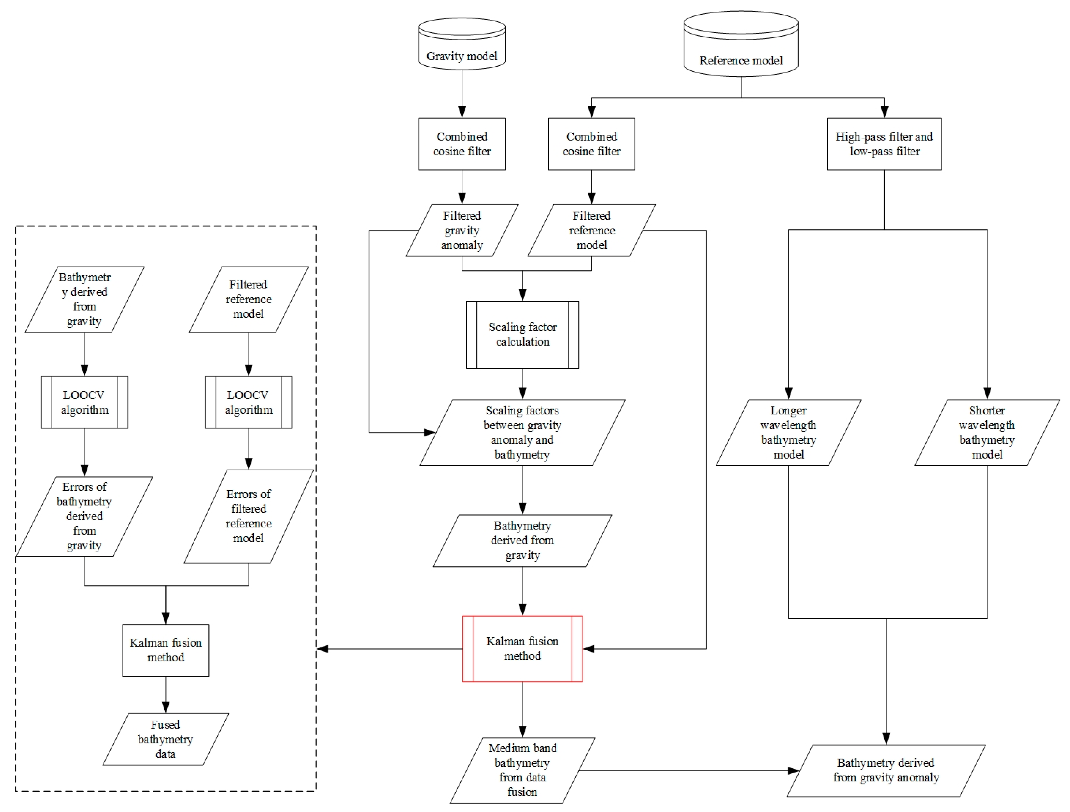
2. Method
2.1. Kalman Fusion Algorithm
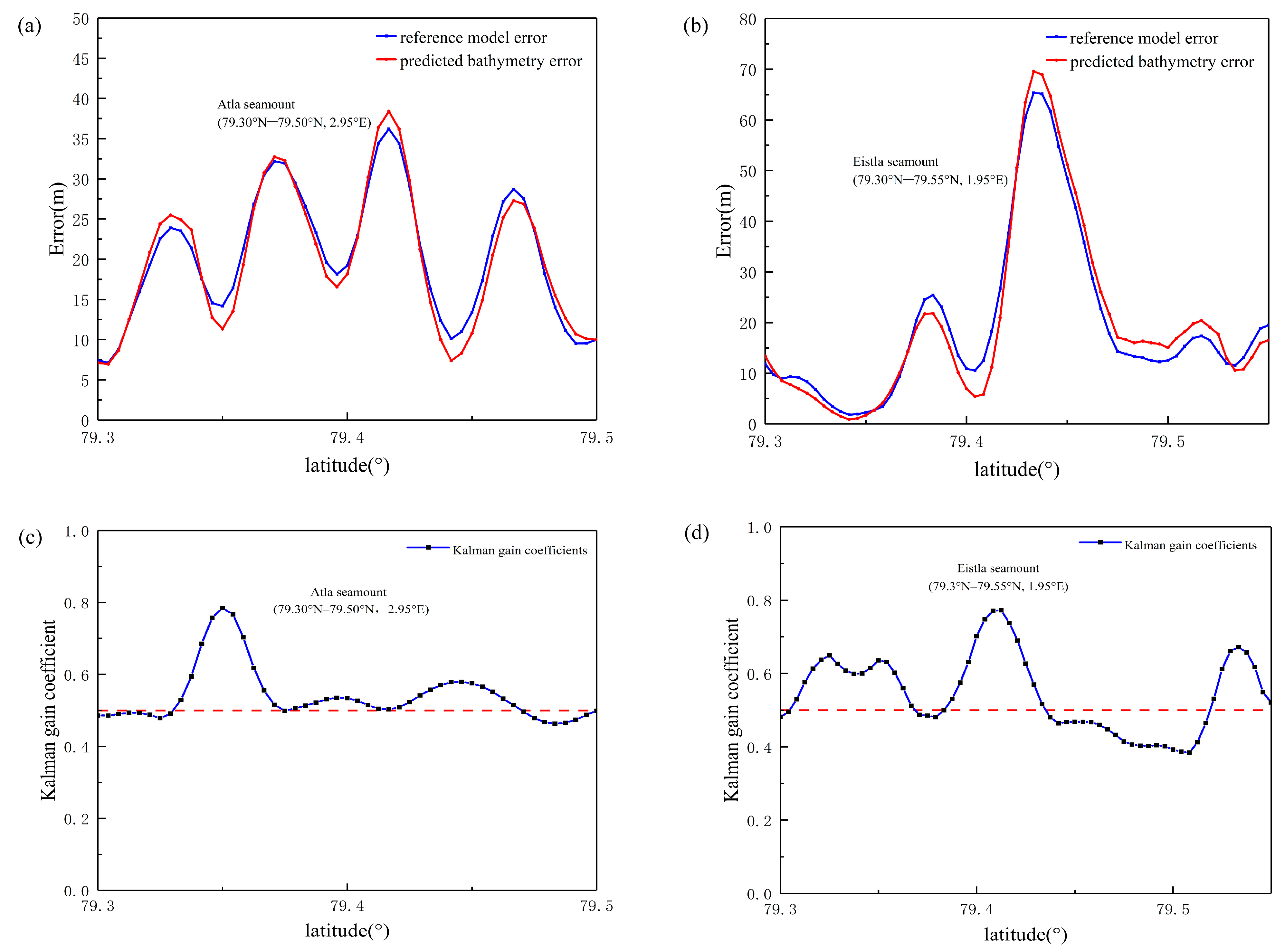
2.2. Computation of Kalman Gain Coefficients
2.3. Estimation of Error of Bathymetry Data
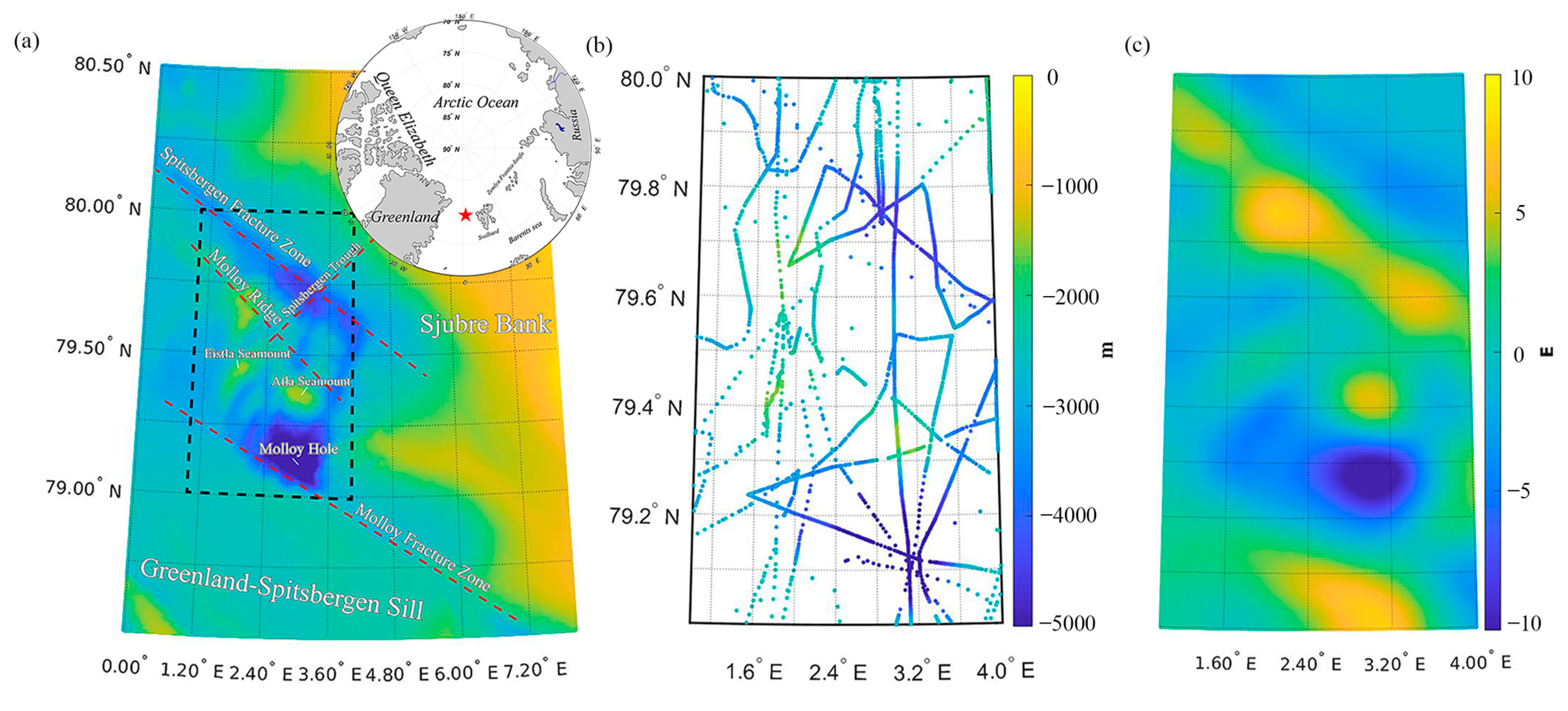
3. Data and Study Area
3.1. Choice of Reference Bathymetry Model
3.2. Altimetric Gravity Models
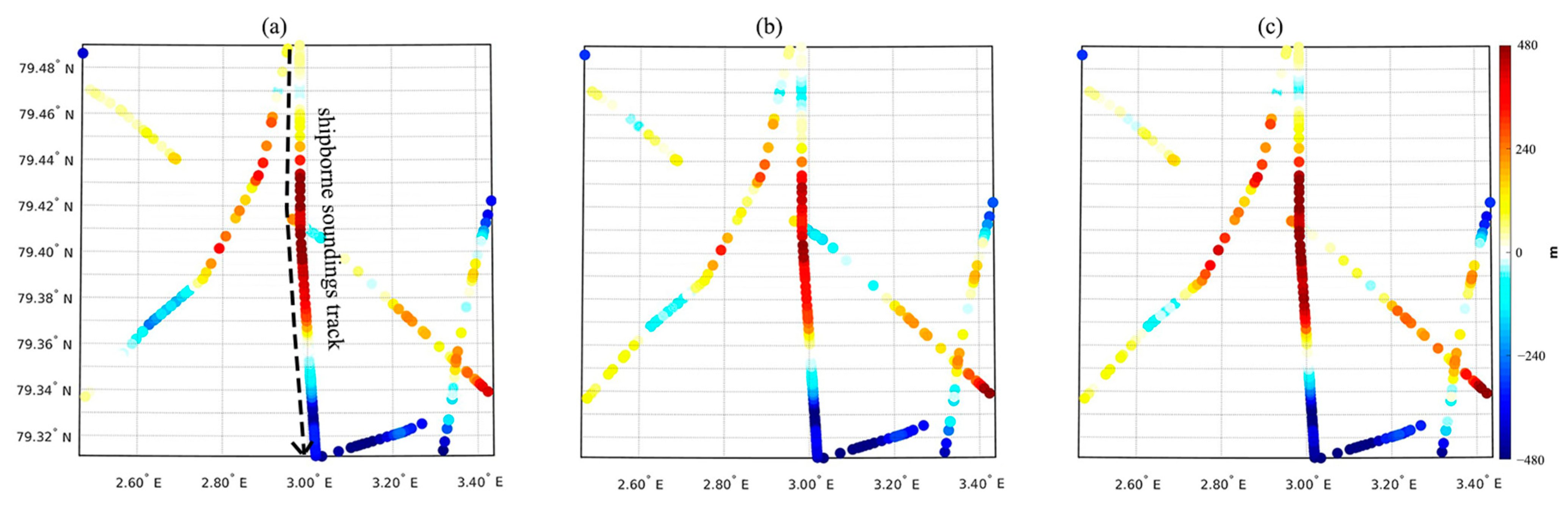
3.3. Shipborne Sounding Data
4. Results and Discussions
4.1. Bathymetry Calculated from Gravity Data
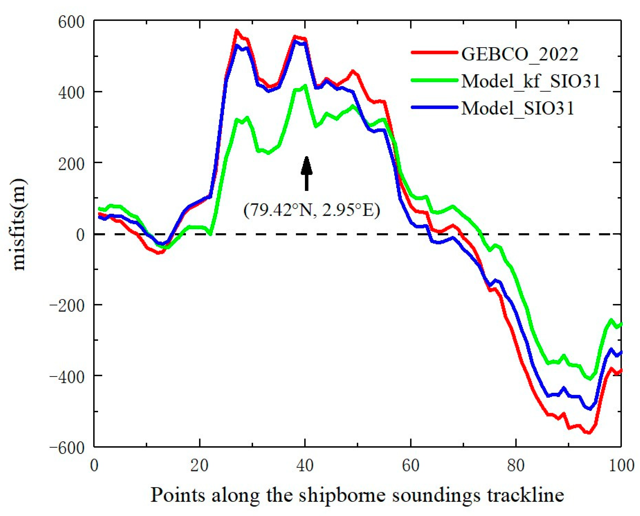
4.2. Bathymetry Modeling from Kalman Fusion Method
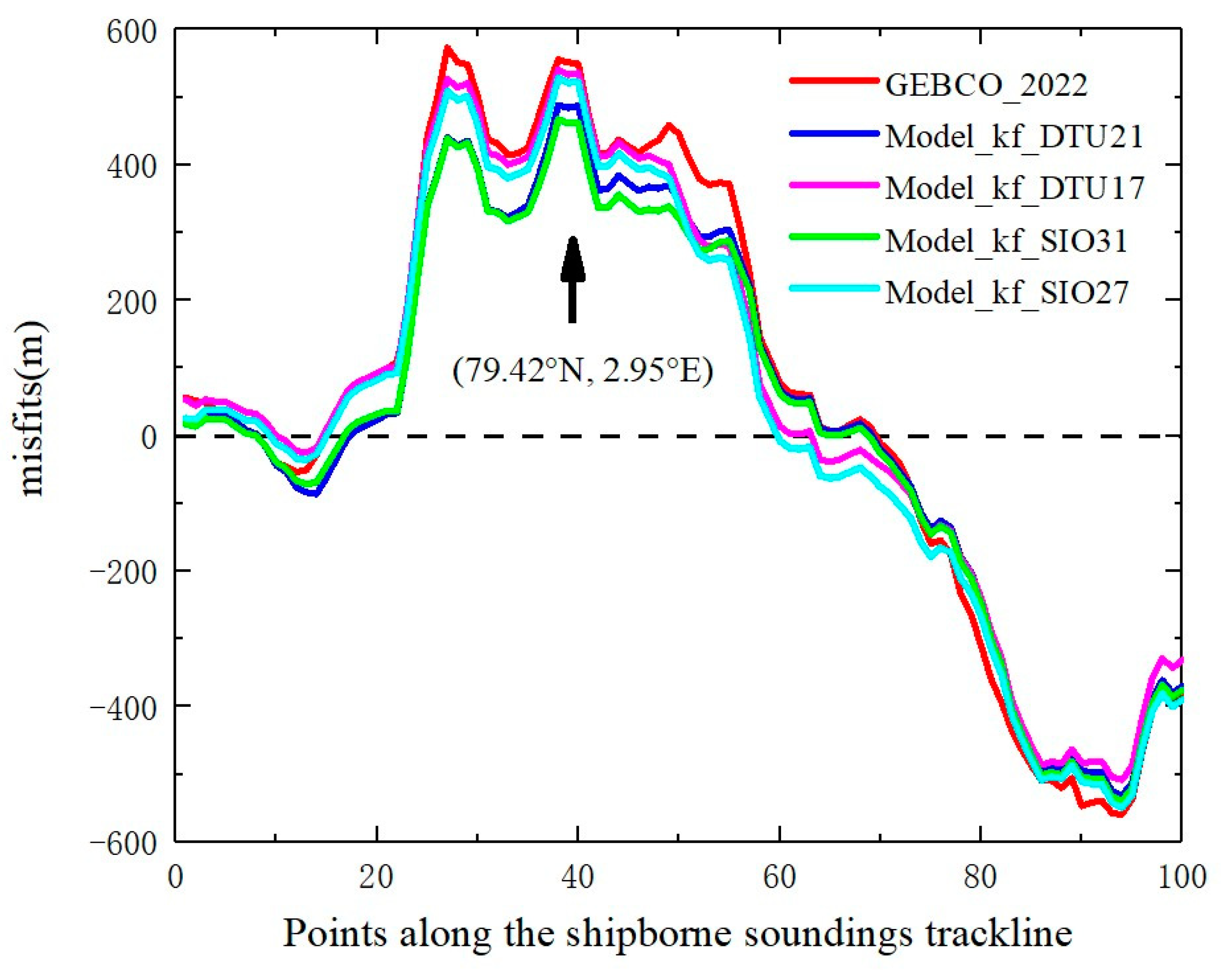
4.3. Comparison of the Results Derived from Different Altimetric Gravity Data
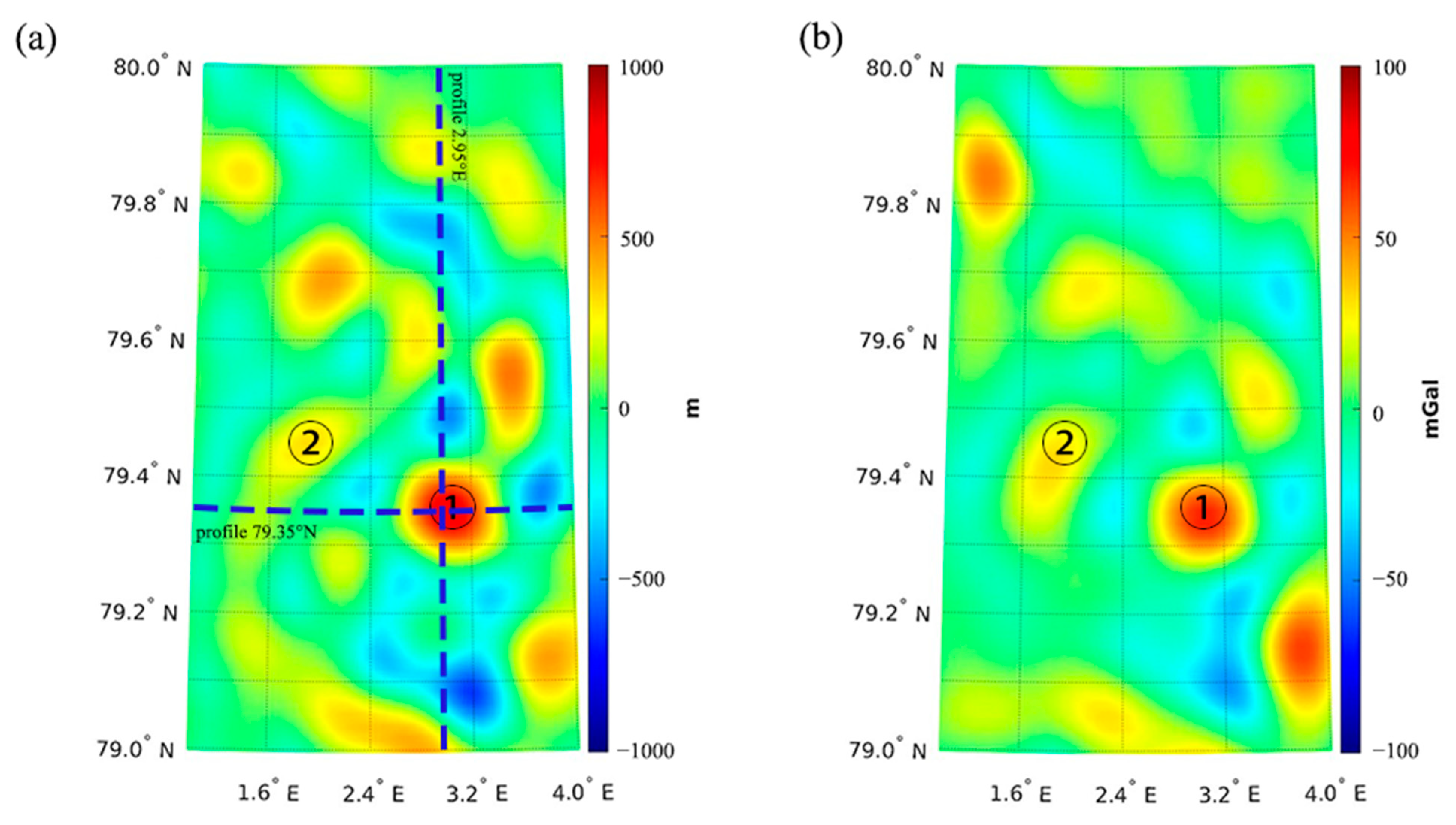
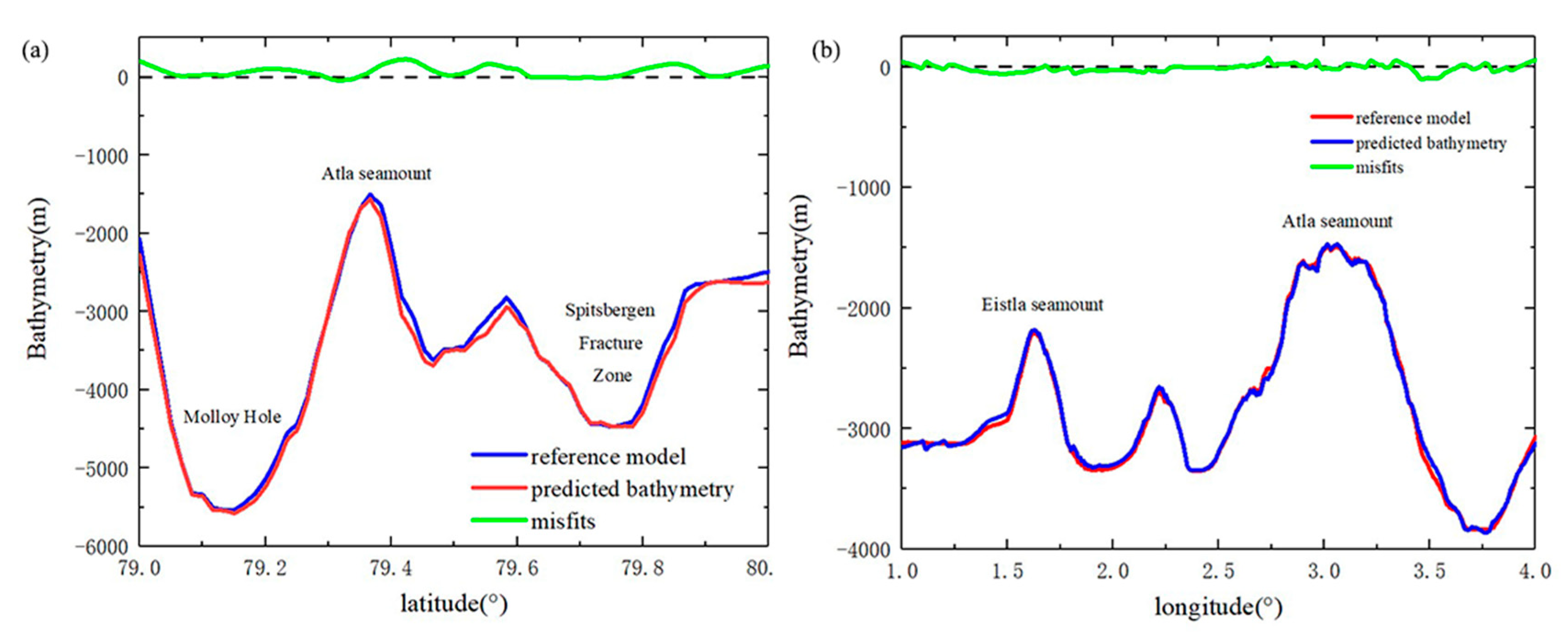
4.3.1. Case Study 1: Atla Seamount
4.3.2. Case Study 2: Eistla Seamount
5. Conclusions
Author Contributions
Funding
Data Availability Statement
Acknowledgments
Conflicts of Interest
References
- Leitner, A.B.; Neuheimer, A.B.; Drazen, J.C. Evidence for long-term seamount-induced chlorophyll enhancements. Sci. Rep. 2020, 10, 1–10. [Google Scholar] [CrossRef]
- Yang, H.; Liu, Y.; Lin, J. Geometrical effects of a subducted seamount on stopping megathrust ruptures. Geophys. Res. Lett. 2013, 40, 2011–2016. [Google Scholar] [CrossRef]
- Jiang, X.; Dong, C.; Ji, Y.; Wang, C.; Shu, Y.; Liu, L.; Ji, J. Influences of Deep-Water Seamounts on the Hydrodynamic Environment in the Northwestern Pacific Ocean. J. Geophys. Res. Oceans 2021, 126, e2021JC017396. [Google Scholar] [CrossRef]
- Weatherall, P.; Marks, K.M.; Jakobsson, M.; Schmitt, T.; Tani, S.; Arndt, J.E.; Rovere, M.; Chayes, D.; Ferrini, V.; Wigley, R. A new digital bathymetric model of the world's oceans. Earth Space Sci. 2015, 2, 331–345. [Google Scholar] [CrossRef]
- Ramillien, G.; Cazenave, A. Global bathymetry derived from altimeter data of the ERS-1 geodetic mission. J. Geodyn. 1997, 23, 129–149. [Google Scholar] [CrossRef]
- Babbel, B.J.; Parrish, C.E.; Magruder, L.A. ICESat-2 Elevation Retrievals in Support of Satellite-Derived Bathymetry for Global Science Applications. Geophys. Res. Lett. 2021, 48, e2020GL090629. [Google Scholar] [CrossRef]
- Watts, A.B.; Tozer, B.; Harper, H.; Boston, B.; Shillington, D.J.; Dunn, R. Evaluation of Shipboard and Satellite-Derived Bathymetry and Gravity Data Over Seamounts in the Northwest Pacific Ocean. J. Geophys. Res. Solid Earth 2020, 125, e2020JB020396. [Google Scholar] [CrossRef]
- Døssing, A.; Hansen, T.; Olesen, A.; Hopper, J.; Funck, T. Gravity inversion predicts the nature of the Amundsen Basin and its continental borderlands near Greenland. Earth Planet. Sci. Lett. 2014, 408, 132–145. [Google Scholar] [CrossRef]
- Childers, V.A.; Brozena, J.M.; Laxon, S.W.; McAdoo, D.C. New gravity data in the Arctic Ocean: Comparison of airborne and ERS gravity. J. Geophys. Res. Solid Earth 2001, 106, 8871–8886. [Google Scholar] [CrossRef]
- Wu, Y.; Abulaitijiang, A.; Andersen, O.B.; He, X.; Luo, Z.; Wang, H. Refinement of Mean Dynamic Topography Over Island Areas Using Airborne Gravimetry and Satellite Altimetry Data in the Northwestern South China Sea. J. Geophys. Res. Solid Earth 2021, 126, e2021JB021805. [Google Scholar] [CrossRef]
- Zhu, C.; Guo, J.; Gao, J.; Liu, X.; Hwang, C.; Yu, S.; Yuan, J.; Ji, B.; Guan, B. Marine gravity determined from multi-satellite GM/ERM altimeter data over the South China Sea: SCSGA V1.0. J. Geodesy 2020, 94, 1–16. [Google Scholar] [CrossRef]
- Galin, N.; Wingham, D.J.; Cullen, R.; Francis, R.; Lawrence, I. Measuring the Pitch of CryoSat-2 Using the SAR Mode of the SIRAL Altimeter. IEEE Geosci. Remote Sens. Lett. 2014, 11, 1399–1403. [Google Scholar] [CrossRef]
- Wu, Y.; Wang, J.; Abulaitijiang, A.; He, X.; Luo, Z.; Shi, H.; Wang, H.; Ding, Y. Local Enhancement of Marine Gravity Field over the Spratly Islands by Combining Satellite SAR Altimeter-Derived Gravity Data. Remote Sens. 2022, 14, 474. [Google Scholar] [CrossRef]
- Parker, R.L. The rapid calculation of potential anomalies. Geophys. J. R. Astron. Soc. 1973, 31, 447–455. [Google Scholar] [CrossRef]
- Hu, M.Z.; Li, J.C.; Li, H.; Shen, C.Y.; Jin, T.Y.; Xing, L.L. Predicting Global Seafloor Topography Using Multi-Source Data. Mar. Geodesy 2014, 38, 176–189. [Google Scholar] [CrossRef]
- Li, Q.Q.; Bao, L.F. Comparative Analysis of Methods for Bathymetry Prediction from Altimeter-derived Gravity Anomalies. Hydrogr. Surv. Charting 2016, 36, 1–4. [Google Scholar]
- Smith, W.H.F.; Sandwell, D. Bathymetric prediction from dense satellite altimetry and sparse shipboard bathymetry. J. Geophys. Res. Solid Earth 1994, 99, 21803–21824. [Google Scholar] [CrossRef]
- Ghorbanidehno, H.; Lee, J.; Farthing, M.; Hesser, T.; Kitanidis, P.K.; Darve, E.F. Novel Data Assimilation Algorithm for Nearshore Bathymetry. J. Atmos. Ocean. Technol. 2019, 36, 699–715. [Google Scholar] [CrossRef]
- Brêda, J.P.L.F.; Paiva, R.C.D.; Bravo, J.M.; Passaia, O.A.; Moreira, D.M. Assimilation of Satellite Altimetry Data for Effective River Bathymetry. Water Resour. Res. 2019, 55, 7441–7463. [Google Scholar] [CrossRef]
- Seoane, L.; Ramillien, G.; Beirens, B.; Darrozes, J.; Rouxel, D.; Schmitt, T.; Salaün, C.; Frappart, F. Regional Seafloor Topography by Extended Kalman Filtering of Marine Gravity Data without Ship-Track Information. Remote Sens. 2021, 14, 169. [Google Scholar] [CrossRef]
- Abulaitijiang, A.; Andersen, O.B.; Sandwell, D. Improved Arctic Ocean Bathymetry Derived from DTU17 Gravity Model. Earth Space Sci. 2019, 6, 1336–1347. [Google Scholar] [CrossRef]
- Tozer, B.; Sandwell, D.T.; Smith, W.H.F.; Olson, C.; Beale, J.R.; Wessel, P. Global Bathymetry and Topography at 15 Arc Sec: SRTM15+. Earth Space Sci. 2019, 6, 1847–1864. [Google Scholar] [CrossRef]
- Kapoor, D.C. General bathymetric chart of the oceans (GEBCO). Mar. Geodesy 1981, 5, 73–80. [Google Scholar] [CrossRef]
- Andersen, O.B.; Knudsen, P. The DTU17 Global Marine Gravity Field: First Validation Results. In International Association of Geodesy Symposia; Springer: Berlin/Heidelberg, Germany, 2019. [Google Scholar]
- Idžanović, M.; Ophaug, V.; Andersen, O.B. Coastal sea level from CryoSat-2 SARIn altimetry in Norway. Adv. Space Res. 2018, 62, 1344–1357. [Google Scholar] [CrossRef]
- Bonnefond, P.; Laurain, O.; Exertier, P.; Boy, F.; Guinle, T.; Picot, N.; Labroue, S.; Raynal, M.; Donlon, C.; Féménias, P.; et al. Calibrating the SAR SSH of Sentinel-3A and CryoSat-2 over the Corsica Facilities. Remote Sens. 2018, 10, 92. [Google Scholar] [CrossRef]
- Donlon, C.; Berruti, B.; Buongiorno, A.; Ferreira, M.-H.; Féménias, P.; Frerick, J.; Goryl, P.; Klein, U.; Laur, H.; Mavrocordatos, C.; et al. The Global Monitoring for Environment and Security (GMES) Sentinel-3 mission. Remote Sens. Environ. 2012, 120, 37–57. [Google Scholar] [CrossRef]
- Sandwell, D.T.; Garcia, E.; Soofi, K.; Wessel, P.; Smith, W.H.F. Towards 1mGal global marine gravity from CryoSat-2, Envisat, and Jason-1. Lead. Edge 2013, 32, 892–899. [Google Scholar] [CrossRef]
- Sandwell, D.T.; Müller, R.D.; Smith, W.H.F.; Garcia, E.; Francis, R. New global marine gravity model from CryoSat-2 and Jason-1 reveals buried tectonic structure. Science 2014, 346, 65–67. [Google Scholar] [CrossRef]
- Sandwell, D.T.; Harper, H.; Tozer, B.; Smith, W.H. Gravity field recovery from geodetic altimeter missions. Adv. Space Res. 2019, 68, 1059–1072. [Google Scholar] [CrossRef]
- Zhao, D.; Wu, Z.; Zhou, J.; Zhang, K.; Luo, X.; Wang, M.; Liu, Y.; Zhu, C. From 10 m to 11000 m, Automatic Processing Multi-Beam Bathymetric Data Based on PGO Method. IEEE Access 2021, 9, 14516–14527. [Google Scholar] [CrossRef]
- Wu, Y.; Wang, J.; He, X.; Wu, Y.; Jia, D.; Shen, Y. Coastal bathymetry inversion using SAR-based altimetric gravity data: A case study over the South Sandwich Island. Geodesy Geodyn. 2022. [Google Scholar] [CrossRef]


| Altimetric Gravity Model | Spatial Resolution | Year of Release | Calculated with SAR Altimeter Data? | Data Set Used in Model Development |
|---|---|---|---|---|
| SIO V23.1 | 2013 | No | This model was calculated by combining data from T/P, Geosat, Envisat, Jason-1, ERS-1/2, and CryoSat-2. | |
| SIO V27.1 | 2018 | No | Introduced more data from Jason-2 and Cryosat-2. | |
| SIO V29.1 | 2019 | Yes | Two years of data from Sentinel-3A/B were added. | |
| SIO V30.1 | 2020 | Yes | Involved data from SARAL/Altika as well as more data from Cryosat-2 and Sentinel-3A/B. | |
| SIO V31.1 | 2021 | Yes | Included more data from Cryosat-2, SARAL/Altika, and Sentinel-3A/B. | |
| DTU15GRA | 2015 | No | This model involved data from CryoSat-2 and Jason-1, and combined data from Topex/Poseidon (T/P), Geosat, ICESat, Jason-1, GFO, Envisat, and retracked data from ERS-1. | |
| DTU17GRA | 2017 | No | Added more CryoSat-2 data and SARAL/AltiKa data from 2016 to 2017 in the geodetic phase. | |
| DTU21GRA | 2021 | Yes | This model added five years of Sentinel-3A and three years of Sentinel-3B compared to DTU17GRA and calculated with reprocessed Cryosat-2 data (processed with the SAMOSA+ physical retracker). |
| Model | Max | Min | Mean | SD |
|---|---|---|---|---|
| Model_kf_SIO31 | 480.99 | −599.39 | −10.33 | 251.91 |
| Model_SIO31 | 542.04 | −582.99 | 8.04 | 261.25 |
| GEBCO_2022 | 572.72 | −602.40 | 22.36 | 286.25 |
| Model | Max | Min | Mean | SD |
|---|---|---|---|---|
| Model_kf_SIO31 | 416.72 | −408.07 | 53.83 | 231.89 |
| Model_SIO31 | 542.04 | −493.08 | 55.84 | 308.04 |
| GEBCO_2022 | 572.72 | −559.24 | 52.75 | 342.32 |
| Model | Max | Min | Mean | SD |
|---|---|---|---|---|
| Model_kf_SIO23 | 529.15 | −614.02 | −2.22 | 267.36 |
| Model_kf_SIO27 | 527.89 | −613.96 | −2.82 | 266.30 |
| Model_kf_SIO29 | 482.08 | −601.25 | −8.72 | 253.52 |
| Model_kf_SIO30 | 482.28 | −599.65 | −8.81 | 253.15 |
| Model_kf_SIO31 | 480.99 | −599.39 | −10.33 | 251.91 |
| Model_kf_DTU15 | 498.26 | −617.12 | −3.94 | 266.18 |
| Model_kf_DTU17 | 519.56 | −594.12 | 11.10 | 263.78 |
| Model_kf_DTU21 | 487.94 | −603.77 | −6.55 | 254.50 |
| GEBCO_2022 | 572.72 | −602.41 | 22.36 | 286.25 |
| Model | Max | Min | Mean | SD |
|---|---|---|---|---|
| Model_kf_SIO23 | 532.00 | −667.10 | −41.30 | 204.87 |
| Model_kf_SIO27 | 529.85 | −647.67 | −43.20 | 202.27 |
| Model_kf_SIO29 | 515.97 | −665.22 | −44.07 | 198.04 |
| Model_kf_SIO30 | 524.49 | −655.99 | −44.58 | 197.85 |
| Model_kf_SIO31 | 519.36 | −657.41 | −46.88 | 197.23 |
| Model_kf_DTU15 | 562.89 | −640.18 | −41.27 | 201.51 |
| Model_kf_DTU17 | 553.17 | −653.87 | −39.11 | 200.33 |
| Model_kf_DTU21 | 525.40 | −659.89 | −48.42 | 196.81 |
| GEBCO_2022 | 529.40 | −640.94 | −20.75 | 215.30 |
Disclaimer/Publisher’s Note: The statements, opinions and data contained in all publications are solely those of the individual author(s) and contributor(s) and not of MDPI and/or the editor(s). MDPI and/or the editor(s) disclaim responsibility for any injury to people or property resulting from any ideas, methods, instructions or products referred to in the content. |
© 2023 by the authors. Licensee MDPI, Basel, Switzerland. This article is an open access article distributed under the terms and conditions of the Creative Commons Attribution (CC BY) license (https://creativecommons.org/licenses/by/4.0/).
Share and Cite
Wu, Y.; Wang, J.; Shen, Y.; Jia, D.; Li, Y. Bathymetry Refinement over Seamount Regions from SAR Altimetric Gravity Data through a Kalman Fusion Method. Remote Sens. 2023, 15, 1288. https://doi.org/10.3390/rs15051288
Wu Y, Wang J, Shen Y, Jia D, Li Y. Bathymetry Refinement over Seamount Regions from SAR Altimetric Gravity Data through a Kalman Fusion Method. Remote Sensing. 2023; 15(5):1288. https://doi.org/10.3390/rs15051288
Chicago/Turabian StyleWu, Yihao, Junjie Wang, Yueqian Shen, Dongzhen Jia, and Yu Li. 2023. "Bathymetry Refinement over Seamount Regions from SAR Altimetric Gravity Data through a Kalman Fusion Method" Remote Sensing 15, no. 5: 1288. https://doi.org/10.3390/rs15051288
APA StyleWu, Y., Wang, J., Shen, Y., Jia, D., & Li, Y. (2023). Bathymetry Refinement over Seamount Regions from SAR Altimetric Gravity Data through a Kalman Fusion Method. Remote Sensing, 15(5), 1288. https://doi.org/10.3390/rs15051288