Article

An Extended Robust Chance-Constrained Power Allocation Scheme for Multiple Target Localization of Digital Array Radar in Strong Clutter Environments

1
Key Laboratory of Radar Imaging and Microwave Photonics, Ministry of Education, Nanjing University of Aeronautics and Astronautics, Nanjing 210016, China
2
Leihua Electronic Technology Research Institute, Aviation Industry Corporation of China, Wuxi 214063, China
*
Author to whom correspondence should be addressed.
Remote Sens. 2023, 15(5), 1267; https://doi.org/10.3390/rs15051267
Submission received: 9 January 2023 / Revised: 19 February 2023 / Accepted: 23 February 2023 / Published: 25 February 2023

Abstract

:
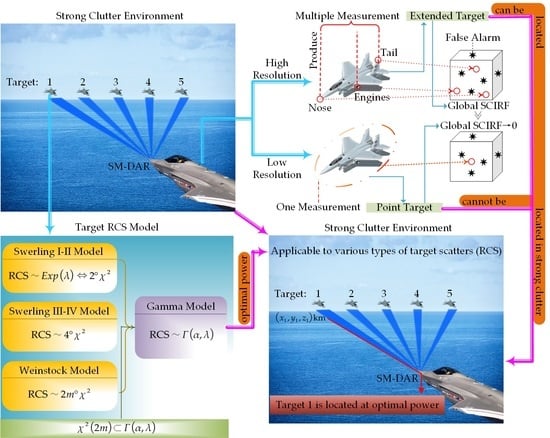
The traditional power allocation method for multi-target localization adopts the Robust Chance Constrained Power Allocation Scheme (RCC-PA), which does not consider the strong clutter characteristics in the current radar detection environment. However, how to reasonably allocate the power required for the radar to locate the target in the strong clutter is a fundamental challenge for improving the combat capability of the radar. Since Simultaneous Multi-beam Digital Array Radar (SM-DAR) can provide high-resolution information on targets in strong clutter, this paper extends the RCC-PA scheme to strong clutter and introduce an extended target model suitable for high-resolution SM-DAR. At the same time, the Gamma distribution is used to reflect the statistical characteristics of the Radar Cross Section (RCS) so that the extended RCC-PA scheme (ERCC-PA) can be suitable for all the scatterers whose RCS belong to Gamma distribution families. In the ERCC-PA scheme, the Strong Clutter Information Reduction Factor (SCIRF) of the extended target is first derived. Then, a Gamma Chance-constraint Programming Model ( Γ -CCP model) is constructed to optimize the power allocation for locating multiple extended targets in strong clutter. The extended dichotomy method for power allocation is also given. Theoretical analysis shows that the power of multi-target localization in strong clutter can still be reasonably allocated under the target with multi-measurement characteristics. In addition, the power distribution of multi-target localization in the strong clutter is negatively correlated with the shape parameter of the Gamma distribution. Specifically, the larger the shape parameter characterizes the larger individual strong scatterer, resulting in the SM-DAR requiring less positioning power. The experimental results verify the theoretical analysis and show that the ERCC-PA scheme can improve the utilization of power compared with the benchmark and has the advantage of robustness to the fluctuation of the target RCS.

Graphical Abstract

1. Introduction

1.1. Background and Motivation

Since the birth of Simultaneous Multi-beam Digital Array Radar (SM-DAR) [1,2,3,4], scholars have favored it because of its unprecedented beam flexibility control and beam combination capabilities, and ability to support various array signal processing algorithms. However, the increasingly complex battlefield situation makes the game between stealth fighters and radar need to consider more detailed factors. For example, the strong clutter will further increase the difficulty of locating targets, and improving the resolution of radar is a means to locate targets effectively. If a high-resolution radar detects a point target, a point target with multiple measurements can be called an extended target according to the characteristic that every part of the point target can be regarded as an effective measurement in this situation. At the same time, each scatterer’s Radar Cross Section (RCS) also fluctuates significantly with different azimuths. Unfortunately, the above factors will affect the transmit power of SM-DAR and make it difficult for the low interception performance of the plane to reach the optimal state while achieving optimal power control is vital in military operations in hostile environments [5]. Therefore, it has become an urgent problem to seek a method that the total transmit power of SM-DAR in strong clutter can also reach the optimal state under the condition of satisfying the localization accuracy requirements and the corresponding power constraints.
When using SM-DAR to locate the target and perform power allocation, it is usually necessary to obtain the lower bound of the estimation error to measure the performance of the filtering algorithm so that the subsequent work can be carried out smoothly. For the estimation of the error lower bound, Tichavsky et al. [6] adopted the Posterior Cramér-Rao Lower Bound (PCRLB) in the 1990s to measure the Mean Square Error (MSE) of discrete-time nonlinear filtering problems. In subsequent studies, PCRLB has been extended to clutter and missed detection [7] and target maneuvering [8]. As far as clutter description is concerned, Information Reduction Factor (IRF), with its unique advantage of being able to integrate all the effects of clutter, has been well applied in estimating the target state and other issues and has become a powerful tool for describing clutter [9,10,11,12,13]. At the same time, with the continuous improvement of radar resolution, the point targets involved in [9,10,11,12,13] will generate multiple measurements simultaneously according to their different reflection points (such as the nose, wing, tail and other parts of the aircraft). With this fundamental change, the algorithm of point targets owning only a single measurement is no longer applicable. Therefore, algorithms for extended targets have been developed successively [14,15,16].
As for the allocation of radar transmit power in the past, in addition to the PCRLB, clutter, and extended target mentioned earlier, RCS’s fluctuation characteristics are also essential factors affecting the quality of the allocation results. In traditional radar resource management research, the RCS of the illuminated target is regarded as a deterministic variable at each moment [17,18,19,20,21,22]. However, in the actual target tracking process, factors such as the target’s identity, attitude, and position often make the RCS at the next sampling moment uncertain [23]. In other words, from the radar point of view, the estimated value of the RCS should have a distribution law. Therefore, many scholars have researched the uncertainty of the target RCS and found that the distribution types of RCS are diverse [24,25,26,27,28]. Specifically, the Swerling I-II, Swerling III-IV, and the Weinstock model can be characterized by exponential ( 2 ° χ 2 ), 4 ° χ 2 , and 2 m ° χ 2 , respectively, where ° represents degrees of freedom, and the χ 2 distribution is a chi-square distribution. Moreover, Refs. [29,30] have contributed significantly to the radar power’s accurate calculation and utilization improvement. In particular, Yan, J. [31] introduced a chance-constrained programming (CCP) model [32] to the problem of locating point targets in a clutter-free environment with 2D SM-DAR and constructed a Robust Chance-Constrained Power Allocation Scheme (RCC-PA scheme). Unlike the previous analysis ideas, Yan J. gave rigorous proof for the first time that the problem to be solved is a convex optimization one and deduced the analytical results of power distribution corresponding to the Swerling I-II model. Among many methods to solve the SM-DAR target localization resource management currently, the RCC-PA scheme is the only method that can give the analytical expression of the power allocation corresponding to the Swerling I-II model. This scheme provides strong support for accurately analyzing the relationship between each parameter and the power distribution result and has broad development prospects.
The above literature shows that the current power allocation problem of target localization considers using SM-DAR to locate point targets in weak clutter and allocate the power of target localization in a way that combines PCRLB and specific RCS distributions. This scenario is quite different from extended target localization in strong clutter, and the distribution of RCS also only involves the exponential distribution ( 2 ° χ 2 distribution) and 4 ° χ 2 distribution in the Swerling I–IV model. However, factors such as strong clutter, extended target, and distribution of RCS will all affect the power allocation of target localization. In particular, with the continuous development of stealth technology, the distribution of the RCS obedience in the previous Swerling I–IV and χ 2 target models cannot be accurately described. In this case, the effect described by a more general distribution may be better and more versatile. Since the exponential distribution ( 2 ° χ 2 distribution), 4 ° χ 2 distribution, and 2 m ° χ 2 distribution obeyed by RCS in the literature [24,27,28] belong to the Gamma distribution family, this paper proposes an extended RCC-PA scheme (ERCC-PA scheme). In the ERCC-PA scheme, the localization of the extended target in strong clutter is closer to the modern radar detection environment. For the convenience of discussion, the CCP model with Gamma distribution type of target RCS in the ERCC-PA scheme is called the Γ -CCP model. The Γ -CCP model can be regarded as the intelligent response of the SM-DAR to multi-target localization by sensing the environment. So far, the problem of power resource allocation can be discussed in a situation that is more in line with the actual detection. Then, the general conclusion of power allocation for locating extended targets in strong clutter when the RCS obeys the Gamma distribution can be obtained so that the ERCC-PA scheme can be appropriately extended at the physical and mathematical levels.

1.2. Major Contributions

The major contributions and innovations of this paper can be classified into the following three points.
  • Aiming at the characteristics of strong clutter in the current detection environment, we propose an ERCC-PA scheme to solve the power allocation problem of high-resolution SM-DAR locating multiple extended targets in strong clutter. This scheme rigorously derives the SCIRF that high-resolution SM-DAR locates multiple extended targets in strong clutter for the first time. On this basis, combined with the Gamma distribution target RCS model suitable for targets with different scattering characteristics, a Γ -CCP model is established to solve the optimal power allocation result. The radar detection environment in the ERCC-PA scheme makes the optimal power allocation of multi-target localization more in line with the actual situation with strong clutter characteristics, and the corresponding analytic method and numerical algorithm have certain reference values for other same type problems.
  • The reason why the high-resolution SM-DAR can reasonably allocate the power of multiple extended target localization in strong clutter is analyzed in detail. The multi-measurement feature of the extended target can increase the number of measurements originating from the real target, thereby greatly enriching the combination between this number and the total number of measurements, and the SCIRF of the extended target is also larger. Since the probability of the number of measurements in the sense of the extended target is greater than that of the point target, the global SCIRF of the extended target by the weighted average of the distribution of the number of measurements will be significantly larger than the global SCIRF of the point target. Therefore, the global SCIRF of the extended target makes it possible for the high-resolution SM-DAR to allocate the power of multi-target localization in strong clutter reasonably.
  • The relationship between the shape parameter and target localization power allocation of target RCS with Gamma distribution law in strong clutter is deeply excavated. At the same confidence level, the power consumption of the target decreases with the increase in the shape parameter. The reason is that when the shape parameter with a larger value causes its cumulative probability to approach 1 to slow down, the probability of RCS taking a larger value in the definition domain will increase, so the negative correlation between RCS and target power consumption makes the relationship between target power consumption and shape parameter also negative correlation. At the same time, the Gamma target model proposed in this paper covers the Swerling I–IV model and the Weinstock model, and the distribution between the generalized chi-square distribution and the Gamma distribution. This type of distribution can often more accurately describe the complex RCS dynamic statistical characteristics of stealth targets, reflecting the universality of the Gamma distribution target model. In addition, from a mathematical point of view, making the RCS obey the Gamma distribution can not only mathematically process many target models uniformly but also physically fit the complex RCS dynamic statistical characteristics of various stealth targets convenient for engineering applications.
The paper’s overall structure is as follows: Section 1 is the introduction. The technical status of the power allocation method for locating multiple extended targets in strong clutter is briefly described. Section 2 is preparatory work. A Gamma target model suitable for various scattering characteristics is given by analyzing the distribution characteristics of RCS in many target models in detail, and the core contents of the measurement model, extended target, and clutter are briefly introduced. Section 3 is the construction of the ERCC-PA scheme, including deriving the analytical expression of the extended target SCIRF, designing the constraints on PCRLB, establishing the Γ -CCP model, and giving the analytic method and numerical algorithm of the model. Section 4 is the simulation experiment. The global SCIRF of the extended target was observed and compared with that of the point target. After verifying the correctness of the analytical results of the global SCIRF of the extended target, the allocation results of the multi-target localization power under the condition that the RCS obeys the Gamma distribution corresponding to different shape parameters are calculated. The relationship between the power distribution results and the shape parameters is summarized on this basis. The last section gives the corresponding conclusions. To clearly show the derivation process of this paper, the naming specification of the symbols in this paper is given in Appendix A.

2. System Model and Preliminaries

Consider an SM-DAR that can be located anywhere x , y , z in three-dimensional space. The system can form multiple simultaneous and independent beams, and each beam illuminates a target. Let k represent the time interval of the kth consecutive frame. Suppose a set is composed of Q extended targets far away from each other, where the target state vector ζ q , k = ( x q , k , y q , k , z q , k , x ˙ q , k , y ˙ q , k , z ˙ q , k ) T , q = 1 , 2 , , Q . The location of the qth target at k time is ( x q , k , y q , k , z q , k ) , and the speed is ( x ˙ q , k , y ˙ q , k , z ˙ q , k ) .

2.1. RCS Model

Assuming that SM-DAR transmits signal s q , k t to target q through the qth beam, and the signal s q , k t has the following form
s q , k t = p q , k S q , k t e j 2 π f c t .
where f c is the carrier frequency and p q , k is the transmission power of target q at time k. The symbol S q , k t represents the normalized complex envelope of the transmitted signal. At the same time, the transmission waveform of the qth beam is assumed to be a narrowband signal with effective bandwidth β q , k [33].
For the received signal from the qth target, its baseband can usually be regarded as the attenuation form of the transmitted signal. Therefore, the received signal with the delay factor τ q , k can be expressed as
r q , k t = h q , k α q , k p q , k S q , k t τ q , k + w q , k t .
where h q , k denotes the reflectivity of the target, the attenuation parameter α q , k 1 / ( D q , k ) 4 is the signal strength change caused by the path loss effect, and D q , k is the distance between the qth target and the radar.
For complex targets, the PDF and the correlation function of RCS are usually difficult to obtain accurately. In this case, a model for estimating the impact of target RCS fluctuation and a method for mathematical analysis came into being. Through the development in recent decades, the models commonly used for the aircraft targets mainly include [34]: Swerling I–IV models, Chi-square ( χ 2 ) target model, Rice target model, and Logarithmic normal target model, and the Swerling I–IV models are all special cases of χ 2 target model. In particular, the freedom degrees of the χ 2 distribution in the target model can be any positive real number, which is slightly different from the rule in probability theory and mathematical statistics that the freedom degrees of the χ 2 distribution must be positive integers. Therefore, the χ 2 distribution in the target model is actually closer to the Gamma ( Γ ) distribution in Probability Theory. Specifically, the χ 2 distribution’s PDF in χ 2 target model has the following form [34]
p σ = m m 1 ! σ a v m σ σ a v m 1 exp m σ σ a v , σ > 0 .
where σ a v is the mean value of RCS. If let m = α and λ = α / σ a v , then Equation (3) can rewritten as
f σ = 1 Γ ( α ) λ α σ α 1 e λ σ , σ > 0 .
Equation (4) is just the PDF of the ( Γ ) distribution in Probability Theory, i.e., when m is not necessarily a positive integer, m corresponds more to the shape parameter α in the Γ distribution.
Ref. [34] shows that the distribution type of RCS in many target models is a member of the gamma distribution family. Therefore, this paper mainly considers the Swerling I–IV and the χ 2 target models and takes the qth target at time k as an example to summarize the relevant distributions’ PDF:
f σ q , k = λ q , k α Γ ( α ) σ q , k α 1 e λ q , k σ q , k , σ q , k > 0 , α R + , Ξ q , k Γ α , λ q , k , 1 / 2 m Γ m σ q , k m 1 e σ q , k 2 , σ q , k > 0 , m R + , Ξ q , k Γ m , 1 2 , 1 2 m m 1 ! σ q , k m 1 e σ q , k 2 , σ q , k > 0 , m Z + , Ξ q , k Γ m , 1 2 χ 2 m , λ q , k e λ q , k σ q , k , σ q , k > 0 , α = 1 , Ξ q , k Γ 1 , λ q , k E x p λ q , k .
where α is the shape parameter and λ q , k is the scale parameter in the Γ distribution.
To be able to see the membership relationship between the four distributions in Equation (5) more intuitively, this paper presents it in the form of a Venn diagram, as shown in Figure 1.
Based on the above analysis, this paper will use the Γ distribution to construct a model for estimating the impact of target fluctuation ( Γ target model). Then, the Γ target model is indeed an appropriate extension of the Swerling I–IV model and χ 2 target model and its scope of application are wider. Therefore, the study of the Γ target model can not only obtain more universal conclusions in theoretical analysis but also achieve better results in practical application, which is of great significance.
To better match the symbols in the text, let h q , k denote the reflectivity of the fluctuating target, then | h q , k | represents the magnitude of the target’s RCS, where | · | is the modulus of “·”. Since | h q , k | 2 is proportional to the reflected power of the illuminated target, ξ q , k = | h q , k | 2 can be used to denote the target’s RCS, which obeys the Γ distribution and its PDF is
f ξ q , k = 1 Γ α λ q , k α ξ q , k α 1 e λ q , k ξ q , k , ξ q , k > 0 .
where λ q , k = α / ξ ¯ q , k , ξ ¯ q , k represents the value obtained by averaging the RCS of all target fluctuations, which is called the mean value of RCS.

2.2. Measurement Model

For the extended target q q = 1 , 2 , , Q , let m q , k be the total number of measurements at time k, and the number of measurements from the target is n q , k . Then, the number of clutter is r q , k = m q , k n q , k . To locate the Q targets mentioned above, SM-DAR generates multiple beams to illuminate them, where each beam has transmission power p q , k . The measurement set can be expressed as
Z q , k = Z q , k i : i = 1 , 2 , , m q , k .
Denote Z ¯ q , k and Z ˜ q , k is the measurement from the target and the false alarm, respectively. The measurement model at time k has the following form
Z q , k i = h q , k ζ q , k + w q , k , Z ¯ q , k i , v q , k , Z ˜ q , k i .
According to Section 1, the SM-DAR has the capability of 4-Dimensional measurement. Thus, the form of h q , k ( ζ q , k ) in Equation (8) is
h q , k ζ q , k = d i a g D q , k , θ q , k , F d q , k , E l q , k .
where D q , k , θ q , k , F d q , k , and E l q , k represent the true distance, azimuth, speed, and pitch measurement of target q, respectively. Moreover, λ ^ q , k is the waverlength of carrier frequency.
Suppose that the measurement error w q , k is a zero-mean uncoupled Gaussian measurement error and has a diagonal covariance matrix R q , k with the form below [23,33]
R q , k = d i a g Var D q , k , Var θ q , k , Var F d q , k , Var E l q , k .
where symbol d i a g · represents diagonal matrix; Var ( D q , k ) , Var ( θ q , k ) , Var ( F d q , k ) , and Var ( E l q , k ) are the errors of the distance, azimuth, speed, and pitch information of the qth target, respectively [23,33].
Var D q , k 1 μ q , k β q , k 2 , Var θ q , k B W μ q , k , Var F d q , k 1 μ q , k T q , k 2 , Var E l q , k B W μ q , k .
where β q , k is the effective bandwidth, B W is the beamwidth of the receiver antenna, T q , k is effective time width, and μ q , k is the signal-to-noise ratio (SNR) of target q whose formula is
μ q , k p q , k ξ q , k D q , k 4 .
By extracting the common factor, the covariance matrix in Equation (10) can be rewritten as
R q , k = 1 p q , k ξ q , k Y q , k .
where Y q , k is a matrix composed of the remaining parameters.

2.3. Theory of Extended Target

The distribution of extended target parameters mentioned in the measurement model is as follows.

2.3.1. Probability Distribution of Z ¯ q , k

According to Equation (8), the measurement error w q , k is zero mean Gaussian white noise and has a diagonal covariance matrix R q , k . Therefore, the measurement Z ¯ q , k obeys the multivariate normal distribution with mean h q , k ( ζ q , k ) and covariance matrix R q , k [35], i.e., Z ¯ q , k i N ( h q , k ( ζ q , k ) , R q , k ) , its PDF is
f T r z ¯ q , k i = 1 | 2 π R q , k | exp 1 2 z ¯ q , k i h q , k ζ q , k T R q , k 1 z ¯ q , k i h q , k ζ q , k .
where z ¯ q , k i is value of Z ¯ q , t i , i.e., F z ¯ q , t T r i = P r Z ¯ q , t i z ¯ q , t i , its dimension is n x , where P r · is probability value, F · is Cumulative Distribution Function (CDF).

2.3.2. Probability Distribution of Measurement Number Originating from Target

In [35], the number n q , k of measurement from targets are assumed to obey the Poisson distribution of the parameter λ ¯ q , k . If the number of measured values from the real target is a random variable Θ q , k , then there is Θ q , k P o i ( λ ¯ q , k ) , and the corresponding probability mass function (PMF) is
p T r n q , k P r Θ q , k = n q , k = λ ¯ q , k n q , k n q , k ! e λ ¯ q , k .

2.4. Theory of Clutter

The distribution of clutter parameters mentioned in the measurement model is as follows.

2.4.1. Spatial Distribution of False Alarm on Clutter

Assuming that the clutter is uniformly distributed in the tracking gate in the observation area A, and the volume of the tracking gate is V q , k . Then, the ith measurement model of the qth target of the clutter is
Z ˜ q , k i = v q , k .
When v q , k A , the PDF of clutter false alarm spatial distribution is
f F a u q , k = 1 V q , k .
Therefore, Z ˜ q , k ( i ) can be regarded as a continuous random variable obeying a uniform distribution U ( V q , k ) with an interval of V q , k .

2.4.2. Number Distribution of False Alarm on Clutter

Generally, the number r q , k of detected false alarms is regarded as obeying the Poisson distribution with the parameter λ ˜ q , k V q , k  [36]. If the number of false alarms is a random variable Υ q , k , then there is Υ q , k P o i ( λ ˜ q , k V q , k ) . The PMF of the number distribution of false alarms is
p F a r q , k P r Υ q , k = r q , k = λ ˜ q , k V q , k r q , k r q , k ! e λ ˜ q , k V q , k .
where λ ˜ q , k is the false alarm density within the target q tracking threshold, and its expression is [37]
λ ˜ q , k = N q , k P f a V q , k .
where N q , k is the total number of irradiation units divided in the tracking gate, and P f a is the false alarm probability.

3. Construction of Extended Robust Chance-Constrained Power Allocation Scheme

In this section, the measurement Z q , k ’s PDF, is derived first. On this basis, a Γ -CCP model is constructed in combination with the uncertain characteristics of RCS to achieve a balance between localization performance and power resources. Finally, the Γ -CCP model is solved by the analytic and double dichotomy (numerical) methods, and the complete ERCC-PA scheme is obtained.

3.1. Derivation of Probability Density Function of Measurement Vector Z q , k

According to Section 2.2, it can be seen that measurement Z q , k has two types of measurements: (1) True measurements produced by the extended target q; (2) False alarms produced by the extended target q. Therefore, the PDF of the measurement Z q , k is jointly determined by three factors: (1) The distribution that the target q is detected; (2) The distribution of the measurement number passing the threshold in the gate; (3) The probability of the existence of the extended target q’s measurements in the measurement Z q , k . By deducing the above three determining factors one by one, the PDF of the measurement Z q , k can be obtained.

3.1.1. Distribution That Target q Is Detected

The result of one detection can be represented by the random variable Λ q , k . Therefore, Λ q , k obeys the Bernoulli distribution with parameter P ¯ d  [12], that is, Λ q , k B e r ( P ¯ d ) , and the corresponding PMF P r Λ q , k = ϖ q , k p D e ϖ q , k is
p D e ϖ q , k = 1 P ¯ d , ϖ q , k = 0 , P ¯ d , ϖ q , k = 1 .

3.1.2. Distribution of Number of Targets Passing Threshold

According to Section 2.3 and Section 2.4, the following proposition can be obtained about the distribution of the number of measurements passing the threshold.
Proposition 1.
Let a random variable  Σ q , k  be the number of measurements passing the threshold in the whole gate, then its PMF  P r Σ q , k = m q , k p T o m q , k  has the following form
p T o m q , k = 1 P ¯ d λ ˜ q , k V q , k m q , k m q , k ! + I 1 m q , k P ¯ d λ ¯ q , k + λ ˜ q , k V q , k m q , k λ ˜ q , k V q , k m q , k m q , k ! e λ ¯ q , k + λ ˜ q , k V q , k .
where  I 1 ( m q , k )  is an indicator function with the form below
I 1 m q , k = 0 , m q , k = 0 , 1 , m q , k > 0 .
Proof. 
When Σ q , k = 0 , there is no over-threshold measurement in the gate, so there are no false alarms and target measurements. Therefore, the following formula holds
P r Σ q , k = m q , k = P r Λ q , k = ϖ q , k P r Υ q , k = r q , k P r Θ q , k = n q , k , m q , k = 0 , ϖ q , k = 0 , r q , k = 0 , n q , k = 0 .
When Σ q , k > 0 , there is an over-threshold measurement within the gate, then the probability without target measurements in this case is
P r Σ q , k = m q , k = P r Λ q , k = ϖ q , k P r Υ q , k = r q , k P r Θ q , k = n q , k , m q , k > 0 , ϖ q , k = 0 , r q , k = m q , k , n q , k = 0 .
If there are target measurements at this time, there is
P r Σ q , k = m q , k = P r Λ q , k = ϖ q , k n q , k = 1 m q , k P r Υ q , k = r q , k P r Θ q , k = n q , k , m q , k > 0 , ϖ q , k = 1 , 0 r q , k = m q , k n q , k < m q , k , 0 < n q , k m q , k .
Through the indicative function I 1 ( m q , k ) of the variable m q , k , that is, Equations (23)–(25) can be expressed in a unified manner by Equation (21), thus, Proposition 1 holds.    □
Therefore, the PMF p T o ( m q , k ) of the number of targets passing the threshold in the wave gate can be regarded as a priori distribution of the number of the target q at time k.

3.1.3. Probability of Measurement Z q , k from Target q

After calculating the distribution of the number of measurements passing the threshold in the gate, the probability of the measurement generated by the target in the measurement Z q , k can be further deduced.
Proposition 2.
Under the condition that there are over-thresholded measurements in the gate, the probability that the measurement  Z q , k  originates from the target has the following expression
ϵ m q , k P r D = P ¯ d p T o m q , k · λ ¯ q , k + λ ˜ q , k V q , k m q , k λ ˜ q , k V q , k m q , k m q , k ! e λ ¯ q , k + λ ˜ q , k V q , k .
where the form of  p T o m q , k  is given by Proposition 1.
Proof. 
If a measurement from target q already exists in measurement Z q , k , the value of m q , k is always greater than zero. Let event A denote that the number of measurements passing the threshold in the gate is Σ q , k = m q , k , and meanwhile let event B denote that there are measurements from the target q under the condition that event A occurs, then the probability of event B occurring can be expressed as
P r B = P r n q , k 0 A = P r 1 n q , k Σ q , k Σ q , k = m q , k = P r 1 n q , k m q , k p T o m q , k .
According to Proposition 1, P r 1 n q , k m q , k has the following form
P r 1 n q , k m q , k = P ¯ d λ ¯ q , k + λ ˜ q , k V q , k m q , k λ ˜ q , k V q , k m q , k m q , k ! e λ ¯ q , k + λ ˜ q , k V q , k .
Combining Equations (27) and (28), the probability of the existence of target q in the measurement Z q , k can be expressed by Equation (26), thus, Proposition 2 holds.    □
So far, the PDF for measurement Z q , k can be obtained by combining Propositions 1 and 2.

3.1.4. Probability Density Function of Measurement

Denote the measurement value vector as Z q , k = Z q , k i : i = 1 , 2 , , m q , k , then the following proposition gives the PDF of measurement Z q , k .
Proposition 3.
Under the premise of given  ζ q , k m q , k  and  n q , k , the PDF of measurement  Z q , k  has the following expression
f z q , k | ζ q , k , m q , k , n q , k = 1 ϵ m q , k V q , k m q , k + 1 Ψ · ϵ m q , k V q , k m q , k n q , k · 1 | 2 π R q , k | n q , k l = 1 Ψ exp i = 1 n q , k 1 2 z ¯ q , k Ψ l i h q , k ζ q , k T R q , k 1 z ¯ q , k Ψ l i h q , k ζ q , k .
where  [ z ¯ q , k ] Ψ l i  represents the value of the ith real measurement corresponding to the l combination under the condition that the combined number is  Ψ .
Proof. 
Let Ψ C m q , k n q , k denote the number of all combinations when there are n q , k real measurements in the m q , k measurement values, then the conditional cumulative distribution function F z q , k ζ q , k , m q , k , n q , k P r Z q , k z q , k ζ q , k , m q , k , n q , k for the measurement Z q , k is
F z q , k | ζ q , k , m q , k , n q , k = 1 ϵ m q , k F z q , k | ζ q , k , all false + ϵ m q , k k = 1 Ψ F z q , k | ζ q , k , Z q , k i = 1 n q , k from target and others from clutter .
If let [ z ¯ q , k ] Ψ l i denote the value of the ith real measurement corresponding to the l combination under the condition that the combined number is Ψ , then according to Propositions 1 and 2, Equations (14), (17), and (30), it can be seen that the conditional PDF for measurement f z q , k ζ q , k , m q , k , n q , k = F z q , k ζ q , k , m q , k , n q , k is
f z q , k | ζ q , k , m q , k , n q , k = 1 ϵ m q , k V q , k m q , k + ϵ m q , k V q , k m q , k n q , k · 1 | 2 π R q , k | n q , k l = 1 Ψ exp i = 1 n q , k 1 2 z ¯ q , k Ψ l i h q , k ζ q , k T R q , k 1 z ¯ q , k Ψ l i h q , k ζ q , k .
Equation (31) can be further written from the normalization property of distribution as Equation (29); thus, Proposition 3 holds.    □

3.2. Evaluation of Multiple Extended Target Localization Performance in Strong Clutter

PCRLB comprises Fisher Information Matrix (FIM), and Conditional FIM (CFIM) is the key to solving FIM. Therefore, this section first deduces the analytical formula of the CFIM in the strong clutter, simplifies the CFIM to solve the FIM in the strong clutter, and finally obtains the corresponding constraints.

3.2.1. Calculation of Conditional Fisher Information Matrix in Strong Clutter

According to the literature [38], the inverse matrix of FIM is PCRLB, and PCRLB can be used as the lower bound of the MSE of the estimated value ζ ^ q , k of the state vector ζ q , k . Therefore, the relationship between the measured MSE and J 1 ( ζ q , k ) is [38]
E ζ q , k , Z q , k , m q , k , n q , k ζ ^ q , k Z q , k ζ q , k ζ ^ q , k Z q , k ζ q , k T J 1 ζ q , k .
where E ζ q , k , Z q , k , m q , k , n q , k · is the expected value with respect to ζ q , k , Z q , k , m q , k , and n q , k .
To deduce the analytical expression of J 1 ( ζ q , k ) , it is necessary first to obtain the data information matrix conditioned on n q , k and m q , k , that is, the expression of CFIM. Hence, there is the following proposition.
Proposition 4.
Under the premise of known  m q , k  and  n q , k , CFIM has the following expression
J k : m q , k : n q , k = E ζ q , k H q , k T Q ^ q , k m q , k , n q , k R q , k 1 H q , k .
where  H q , k ζ q , k T h q , k ( ζ q , k )  is the Jacobian matrix of  n z  row and  n x  column, and the form of  Q ^ m q , k , n q , k  is
Q ^ q , k m q , k , n q , k = E ζ q , k β Z q , k , ζ q , k 2 R q , k 1 l 1 = 1 Ψ l 2 = 1 Ψ φ z ¯ q , k Ψ ( l 1 ) i φ z ¯ q , k Ψ ( l 2 ) j T ζ q , k , l n = 1 , 2 , , Ψ ; n = 1 , 2 .
In  Q ^ m q , k , n q , k , parameters  β Z q , k , ζ q , k φ z ¯ q , k Ψ l i , and  H Ψ k i  have the following forms
β Z q , k , ζ q , k = 1 f z q , k | ζ q , k , m q , k , n q , k · ϵ m q , k Ψ V q , k m q , k n q , k · 1 | 2 π R q , k | n q , k , φ z ¯ q , k Ψ l i = i = 1 n q , k H Ψ l i exp i = 1 n q , k 1 2 H Ψ l i T R q , k 1 H Ψ k i . H Ψ k i = z ¯ q , k Ψ k i h q , k ζ q , k ,
respectively.
Proof. 
According to the method in [6], it can be known that
J k : m q , k : n q , k = E ζ q , k , Z q , k ln f z q , k | ζ q , k ζ q , k ln f z q , k | ζ q , k ζ q , k T m q , k , n q , k , = E ζ q , k , Z q , k [ ln f z q , k | ζ q , k , m q , k , n q , k ζ q , k Δ ln f z q , k | ζ q , k , m q , k , n q , k ln f z q , k | ζ q , k , m q , k , n q , k ζ q , k T ] .
Combining Proposition 3 with the chain rule of function derivation, Δ ln f ( z q , k | ζ q , k , m q , k , n q , k ) has the following form
Δ ln f ( z q , k | ζ q , k , m q , k , n q , k ) = 1 f z q , k | ζ q , k , m q , k , n q , k · f z q , k | ζ q , k , m q , k , n q , k ζ q , k = 1 f z q , k | ζ q , k , m q , k , n q , k · ϵ m q , k Ψ V q , k m q , k n q , k · 1 | 2 π R q , k | n q , k · l = 1 Ψ { exp i = 1 n q , k 1 2 H Ψ l i T R q , k 1 H Ψ l i · i = 1 n q , k { H Ψ l i ζ q , k T T · 1 2 H Ψ l i T R q , k 1 H Ψ l i H Ψ l i } } .
where H Ψ k i = z ¯ q , k Ψ k i h q , k ζ q , k . Then according to the chain rule of matrix derivation, we can get
H Ψ l i ζ q , k T T = H q , k T , 1 2 H Ψ l i T R q , k 1 H Ψ l i H Ψ l i = R q , k 1 H Ψ l i .
Therefore, Equation (37) can be written as
Δ ln f ( z q , k | ζ q , k , m q , k , n q , k ) = 1 f z q , k | ζ q , k , m q , k , n q , k · ϵ m q , k Ψ V q , k m q , k n q , k · 1 | 2 π R q , k | n q , k · l = 1 Ψ exp i = 1 n q , k 1 2 H Ψ l i T R q , k 1 H Ψ l i H q , k T R q , k 1 i = 1 n q , k H Ψ l i .
If let
β Z q , k , ζ q , k = 1 f z q , k | ζ q , k , m q , k , n q , k · ϵ m q , k Ψ V q , k m q , k n q , k · 1 | 2 π R q , k | n q , k , φ [ z ¯ q , k ] Ψ l i = i = 1 n q , k H Ψ l i exp i = 1 n q , k 1 2 H Ψ l i T R q , k 1 H Ψ k i .
then Equation (39) can be transformed into the following simplest form
Δ ln f ( z q , k | ζ q , k , m q , k , n q , k ) = β Z q , k , ζ q , k H q , k T R q , k 1 l = 1 Ψ φ z ¯ q , k Ψ l i .
Hence, the form of CFIM will be further expressed as
J k : m q , k : n q , k = E ζ q , k E Z q , k β Z q , k , ζ q , k H q , k T R q , k 1 k = 1 Ψ φ z ¯ q , k Ψ k i · k = 1 Ψ φ z ¯ q , k Ψ k i T R q , k 1 H q , k β Z q , k , ζ q , k ζ q , k , = E ζ q , k H q , k T Q ^ q , k m q , k , n q , k R q , k 1 H q , k .
where the expression of Q ^ q , k ( m q , k , n q , k ) is
Q ^ q , k m q , k , n q , k = E ζ q , k β Z q , k , ζ q , k 2 R q , k 1 l 1 = 1 Ψ l 2 = 1 Ψ φ z ¯ q , k Ψ ( l 1 ) i φ z ¯ q , k Ψ ( l 2 ) j T ζ q , k , l n = 1 , 2 , , Ψ ; n = 1 , 2 .
Thus, Proposition 4 holds.    □
According to the derivation process of the point target’s CFIM [12], Q ^ q , k ( m q , k , n q , k ) can be called the Information Reduction Factor Matrix in strong clutter. As can be seen from Equation (38), when the combination number is Ψ , each value of l n n = 1 , 2 corresponds to a combination form. Then, l n n = 1 , 2 can be regarded as a combination number, which is called a combination number variable for short, that is, l n n = 1 , 2 traverses all combination cases. At the same time, l 1 and l 2 are independent of each other.

3.2.2. Calculation of Fisher Information Matrix in Strong Clutter

When Q ^ q , k ( m q , k , n q , k ) is independent of ζ q , k , Q ^ q , k ( m q , k , n q , k ) is a constant IRF [12]. In this case, the final form of CFIM can be obtained by simplifying Q ^ q , k ( m q , k , n q , k ) , and then FIM can be obtained. Thus, there is the following proposition.
Proposition 5.
Under the condition that  Q ^ q , k ( m q , k , n q , k )  is independent of  ζ q , k , FIM has the following expression
J ( ζ q , k ) = ϕ q , k · E ζ q , k [ ( H q , k ) T R q , k 1 H q , k ] .
where
ϕ q , k = m q , k = 1 p T o ( m q , k ) n q , k = 1 m q , k [ P r ( n q , k | m q , k ) q ^ q , k ( m q , k , n q , k ) ] .
is the global SCIRF of the extended target, and
q ^ q , k m q , k , n q , k = Π m q , k , n q , k Ψ 2 ( V q , k ) 2 r q , k · ϵ m q , k 2 R q , k 0.5 m q , k n q , k 2 π n x n q , k g g g g n q , k × n x g g g g r q , k × n x { z ¯ q , k 1 a 2 exp n q , k i = 1 n x z ¯ q , k 1 i 2 } / { 1 ϵ m q , k ( V q , k ) m q , k + 1 Ψ · ϵ m q , k ( V q , k ) r q , k | 2 π R q , k | n q , k k = 1 Ψ exp { r = 1 n q , k 1 2 i = 1 n x z ¯ q , k Ψ k r i } d z ¯ q , k 1 d z ¯ q , k n q , k d z ˜ q , k 1 d z ˜ q , k r q , k
is the SCIRF of the extended target, and the even symmetric term coefficient  Π m q , k , n q , k  has the form
Π m q , k , n q , k = l = 0 n q , k n q , k l C m q , k n q , k l C r q , k + l l C r q , k l , n q , k m q , k 1 / 2 , l = 0 m q , k 1 / 2 l 1 * + 1 n q , k l C m q , k n q , k l C r q , k + l l C r q , k l , n q , k = m q , k 1 / 2 + l 1 * , n q , k , n q , k = m q , k . m q , k = 2 n 1 , n N + , l 1 * = 1 , 2 , , m q , k 1 / 2 .
Π m q , k , n q , k = l = 0 n q , k n q , k l C m q , k n q , k l C r q , k + l l C r q , k l , n q , k m q , k / 2 , l = 0 m q , k / 2 l 2 * n q , k l C m q , k n q , k l C r q , k + l l C r q , k l , n q , k = m q , k 1 / 2 + l 2 * , n q , k , n q , k = m q , k . m q , k = 2 n , n N + , l 2 * = 1 , 2 , , m q , k / 2 1 .
z ¯ q , k r i  represents the normalized variable of the ith dimension information of the rth measurement of the target q at time k.
Because the proof process of Proposition 5 is rather tedious, this paper moves this part to Appendix B.

3.2.3. Constraints Construction of Pcrlb for Multi-Target Localization in Strong Clutter

As seen from Section 3.2.1, as the inverse matrix of FIM, PCRLB enables one to determine the lower bound of the best achievable accuracy of target localization estimation. Therefore, we use PCRLB to represent the localization MSE and serve as a constraint function for the ERCC-PA scheme.
To meet the real-time requirements, Equation (13) is substituted into Equation (44) for calculation, and the expression of the FIM about the target RCS variable ξ q , k and the transmit power p q , k can be obtained
J ζ q , k = ϕ q , k p q , k ξ q , k H q , k T Y q , k 1 H q , k .
For power allocation, For power allocation, to meet the localization accuracy requirements of target q, F p q , k , ξ q , k needs to meet the condition that it does not exceed the required localization threshold η q , k . The trace of the PCRLB matrix is used as an index to measure the localization performance [1], so there is the following equation
F p q , k , ξ q , k = tr PCRLB p q , k , ξ q , k ζ q , k = tr ϕ q , k p q , k ξ q , k A q , k η q , k .
where
A q , k = H q , k T Y q , k 1 H q , k
Let the characteristic polynomial of matrix A q , k contain m ^ ( m ^ < n ) multiple roots (when m ^ = 0 , there are no multiple roots). If the number of multiple roots λ i ( i = 1 , 2 , , m ^ ) is r i , then according to Jordan’s theorem, Equation (50) can be transformed into
F p q , k , ξ q , k = 1 ϕ q , k p q , k ξ q , k i = 1 m ^ r i λ i + i = m ^ + 1 n 1 λ i η q , k .
If let
ς q , k = 1 ϕ q , k η q , k i = 1 m ^ r i λ i + i = m ^ + 1 n 1 λ i .
then the inequality constraint in Equation (52) can be rewritten as follows
ξ q , k ς q , k p q , k .
Equation (54) is the constraint condition of multi-target localization PCRLB in strong clutter.

3.3. Gamma Chance-Constrained Programming Model

In the Γ -CCP model, ξ q , k in Equation (54) is regarded as a random variable of the target RCS. For the target RCS model in Equation (6), a chance-constrained programming problem to minimize the total transmit power of SM-DAR is established in this paper. In this case, SM-DAR can meet specific multi-target localization accuracy requirements with a predetermined confidence level 1 δ . The Γ -CCP model is shown below
min p k 1 T p k s . t . P r F p 1 , k , ξ 1 , k η 1 , F p 2 , k , ξ 2 , k η 2 , , F p Q , k , ξ Q , k η Q 1 δ , p q , k 0 , q = 1 , , Q
where p k = p 1 , k , p 2 , k , , p Q , k T is the adaptive transmit power vector and P r · is the probability of the random RCS ξ q , k .
In the actual scenario, for any two aircraft (target) of different beams, their respective flight status does not affect each other’s flight statuses. Therefore, there is the following assumption.
Assumption 1.
The target  q q = 1 , 2 , , Q ’s RCS variable  ξ 1 , k , ξ 2 , k , , ξ Q , k  is a sequence of independent and identically distributed (i.i.d) random variables, which is denoted as  { ξ i , k , i Z + } .
According to Assumptions 1, the multi-target joint constraint function can be expressed as the product of constraint functions corresponding to different targets. In this case, by substituting Equation (54) into the first constraint of the problem (55), the problem (55) can be rewritten as
min p k 1 T p k s . t . q = 1 Q P r ξ q , k ς q , k p q , k 1 δ , p q , k 0 , q = 1 , , Q .
where the PDF of the RCS is Equation (6). For each target, its complementary cumulative distribution function can be calculated as
P r ξ q , k ς q , k p q , k = ς q , k p q , k + f ξ q , k d ξ q , k = 1 Γ α Γ α , λ q , k ς q , k p q , k .
where Γ α is the Gamma function with parameter α , and Γ α , λ q , k ς q , k / p q , k is the upper incomplete Gamma function with parameters α and λ q , k ς q , k / p q , k .
Substituting Equation (57) into the first inequality constraint of Equation (56) and taking the natural logarithms on both sides at the same time, the inequality constraint can be rewritten as
q = 1 Q ln 1 Γ α Γ α , λ q , k ς q , k p q , k b .
where b = ln 1 δ . Hence, problem (55) can be expressed equivalently as follows
min p k 1 T p k s . t . q = 1 Q f ^ q , k p q , k b , f ^ q , k p q , k = ln 1 Γ α Γ α , λ q , k ς q , k p q , k p q , k 0 , q = 1 , , Q .
where the f ^ q , k p q , k , q = 1 , , Q of all targets is continuously differentiable functions. The convexity proof of the optimization problem is shown in Appendix C.

3.4. Solution of Γ-CCP Model

According to Section 2.1, the type of RCS model is determined by the shape parameter α of the Gamma distribution. For the convenience of subsequent discussion, starting from this section, the function f ^ q , k p q , k is written as f ^ q , k p q , k ; α to distinguish the conclusions corresponding to different RCS models.

3.4.1. Equivalent Representation of Problem

If p q , k meets the following conditions [31]
f ^ q , k p q , k ; α = ϑ , ϑ > 0 , q = 1 , , Q , q = 1 Q f ^ q , k p q , k ; α = b .
problem (59) has the optimal solution. In this case, let p q , k p q , k opt and the optimal solution p k opt = [ p 1 , k opt , p 2 , k opt , , p q , k opt ] T , the problem (59) can be rewritten to
find ϑ , p k s . t . f ^ q , k 1 ϑ ; α = p q , k , q = 1 , , Q , q = 1 Q f ^ q , k p q , k ; α = b .
On this basis, by substituting Equations (A24) and (A27) into the first constraint in problem (61), the following polynomial equation can be obtained
λ q , k ς q , k α 1 p q , k 2 λ q , k ς q , k α ϑ + i = 1 α 1 α i p q , k α + 1 + i = 2 α 1 λ q , k ς q , k α i p q , k 1 + i j = 1 i 1 α j = 0 .
After obtaining the relational expression p q , k = f ^ q , k 1 ϑ ; α from Equation (62), it is substituted into the second constraint in problem (61), and the optimal value ϑ opt of ϑ can be obtained. Further, the optimal power allocation result p k opt can be obtained by substituting ϑ opt into the first constraint in problem (61). Therefore, the analytical solution of p k opt can only be obtained when both constraints in problem (61) have analytical solutions.
Without loss of generality, this paper takes α = 1 , 2 , 3 , 4 as an example and shows the types of the two constraints and the existence of the analytical solution of p k opt in Table 1 below.
Combining Table 1 and the Cardano formula and Ferrari method root formula, the constraint condition p q , k = f ^ q , k 1 ϑ ; α has theoretically rooted formula solutions in Case1, Case2, and Case3. However, only the function f ^ q , k p q , k ; α in Case1 is not a transcendental function. Therefore, p k opt has an analytical solution only in Case1.
Given this, the analytical solution of p k opt is given first in the next section, and an extended numerical algorithm is given on this basis.

3.4.2. Analytic Solution and Numerical Solution of Γ -CCP Model

According to the solution process mentioned in Section 3.4.1, the optimal power analytical expression of Case1 in the ERCC-PA scheme is
p k opt = λ 1 , k ς 1 , k · q = 1 Q λ q , k ς q , k b , λ 2 , k ς 2 , k · q = 1 Q λ q , k ς q , k b , , λ Q , k ς Q , k · q = 1 Q λ q , k ς q , k b T .
It can be seen from Equation (63) that p q , k opt is proportional to the scale parameter λ q , k of the RCS of the target q. At the same time, it can be known from Equations (53) and (58) that ς q , k is inversely proportional to ϕ q , k , and b is proportional to 1 δ . Therefore, p q , k opt is inversely and directly proportional to ϕ q , k and 1 δ , respectively.
For the case of α 2 , it needs to be calculated by numerical method. Unlike the literature [31], the power of the variable p q , k in the constraint condition ϑ = f ^ q , k ( p q , k ; α ) in this paper is no longer limited to 3. When the power of the polynomial equation is greater than 5, Abel’s theorem indicates that the equation has no root formula solution, so it is necessary to expand the numerical algorithm of literature [31]. Considering that the constraint condition ϑ = f ^ q , k ( p q , k ; α ) is always monotonically increasing for p q , k , the functions y = f ^ q , k ( p q , k ; α ) and y = ϑ have only one intersection point, that is, the only zero point. Similarly, y = f ^ q , k ( p q , k ; α ) and y = b / Q have only one zero point. Therefore, the idea of dichotomy in numerical analysis can still be used for reference, i.e., a simple attempt is made in the domain, the upper and lower bounds of the zero point are determined, and then the zero point is continuously approached through iteration. Algorithm 1 shows the detailed steps of the extended numerical algorithm.
Algorithm 1: Detailed steps of the extended numerical algorithm
Remotesensing 15 01267 i001
Based on the above analysis, the next section conducts simulation experiments on the solution of the Γ -CCP model to further discuss the effectiveness and robustness of the ERCC-PA scheme.

4. Simulation

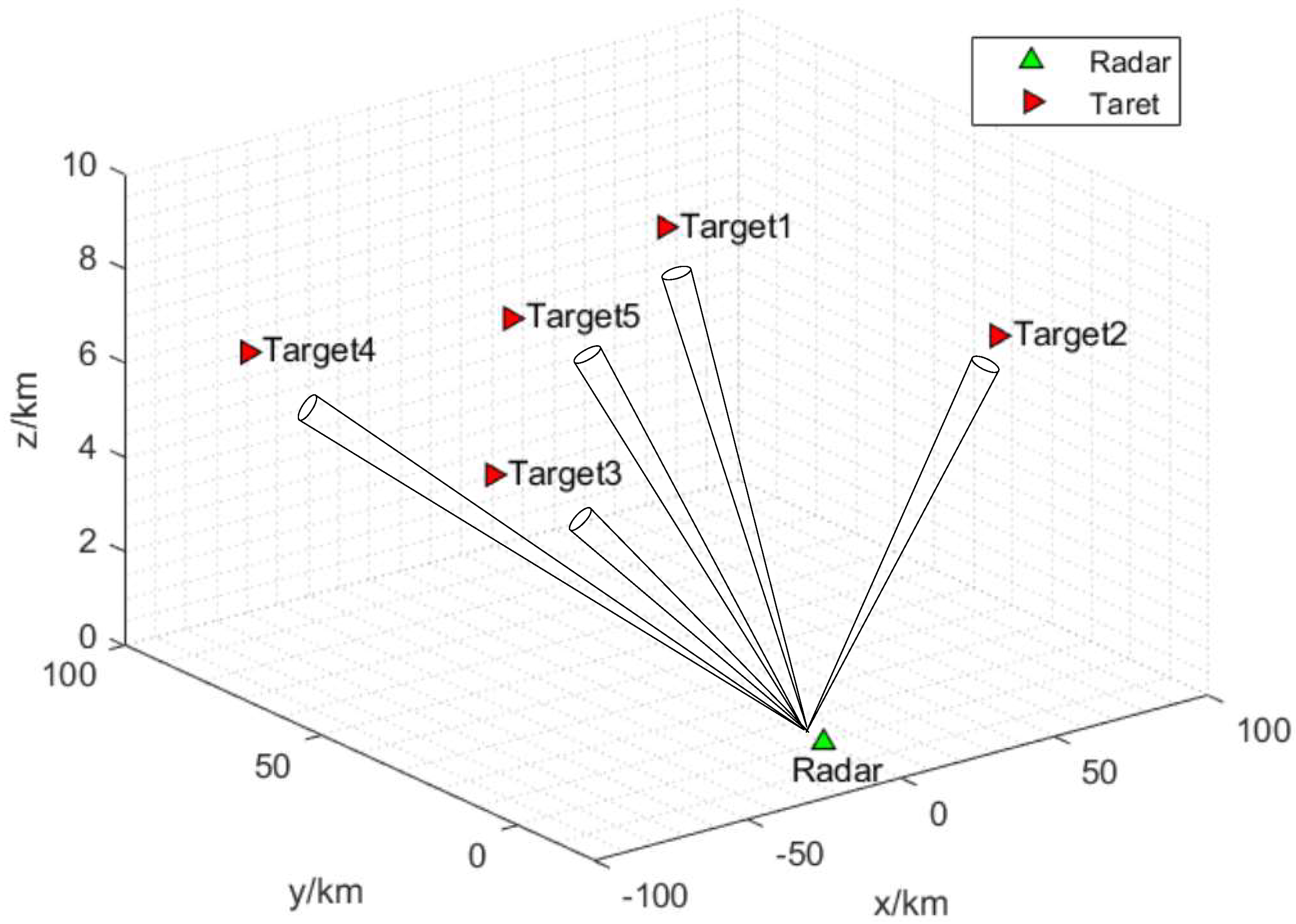
Consider a SM-DAR arbitrarily located at 0 , 0 , 1 km . Figure 2 shows the deployment of the extended target with respect to the SM-DAR. The radar adopts the SM operation mode of synchronous multi-beam synthesis, and each beam is used to illuminate the specified target.
Before the simulation experiment, the radar parameter values are given in Table 2. At the same time, Table 3 shows each target’s location, distance, localization accuracy threshold, and expectation of RCS. According to Table 3, Target 5 has the shortest distance from SM-DAR, the largest mean value of its corresponding RCS, and the best observation conditions.
In this section, the relationship between SCIRF and various parameters is first discussed and analyzed. Then, Case1 is used as an example to verify the correctness of the double dichotomy. Finally, the method is used in the solution process of Case2, Case3, and Case4 to verify the validity and robustness of the ERCC-PA scheme.

4.1. Information Reduction Factor in Clutter

In this section, target one is taken as an example without loss of generality. The relationship among other parameters under the same clutter density and the relationship between different clutter densities and various parameters is quantitatively analyzed for the case of point target and extended target. On this basis, taking Case1 as an example, the power distribution of target positioning under different clutter densities is compared.
For the convenience of subsequent discussion, a distinction is made here between the symbolic representations of the point target and extended target parameters. Still, take target one as an example. For the probability ϵ ( m 1 , k ) corresponding to the presence of a measurement Z ¯ 1 , k from the real target in the measurement Z 1 , k , if Z ¯ 1 , k is the measurement generated by the point target, then ϵ ( m 1 , k ) can be denoted as ϵ ˙ ( m 1 , k ) . If Z ¯ 1 , k is the measurement generated by the extended target, then ϵ ( m 1 , k ) may be denoted as ϵ ¨ ( m 1 , k ) . For the global IRF of the target, if the target is regarded as a point target, then ϕ 1 , k can be denoted as ϕ ˙ 1 , k , called the point target global IRF. If the target is regarded as an extended target, then ϕ 1 , k can be denoted as ϕ ¨ 1 , k , called the extended target global SCIRF. In addition, if the difference between high and low clutter environments needs to be reflected, ϵ ¨ ( m 1 , k ) can be written as ϵ ¨ H ( m 1 , k ) and ϵ ¨ L ( m 1 , k ) , and ϕ ¨ 1 , k can be written as ϕ ¨ 1 , k , H and ϕ ¨ 1 , k , L . Similar distinctions can be made for other parameters.

4.1.1. Calculation of Scirf Based on Monte Carlo Method

According to the analysis in Section 4.1.1, it can be seen that the point target’s IRF q ^ ˙ q , k ( m q , k , n q , k ) is comparable to the extended target’s SCIRF q ^ ¨ q , k ( m q , k , n q , k ) when n q , k = 1 . Therefore, the similarities and differences between q ^ ˙ q , k ( m q , k , n q , k ) and q ^ ¨ q , k ( m q , k , n q , k ) under the condition of n q , k = 1 are discussed in this section.
Because the form of the extended target’s SCIRF q ^ ¨ q , k ( m q , k , n q , k ) in Equation (A14) is very complex and its multiple integral values by both analytic and numerical methods are difficult to obtain, this paper adopts the Monte Carlo simulation method to solve this problem. Through the Monte Carlo method, q ^ ¨ q , k ( m q , k , n q , k ) can be written as
q ^ ¨ q , k ( m q , k , n q , k ) = Π m q , k , n q , k · 2 g m q , k n x · 1 Ψ 2 · ϵ ¨ m q , k 2 ( V q , k ) 2 r q , k · R q , k 0.5 m q , k n q , k 2 π n x n q , k · 1 N M C r = 1 N M C U 1 , 1 r 2 exp n q , k j = 1 n x U 1 , j r 2 / { 1 ϵ ¨ m q , k ( V q , k ) m q , k + 1 Ψ · ϵ ¨ m q , k ( V q , k ) r q , k · 1 | 2 π R q , k | n q , k k = 1 Ψ exp l = 1 n q , k 1 2 i = 1 n x U l , i Ψ k r 2 .
where N M C is the Monte Carlo simulation times, U l , i r ( l = 1 , , m q , k ; i = 1 , , n x ; r = 1 , , N s ) is a continuous random variable with independent and identically distributed, and U l , i r obeys the uniform distribution with interval g , g .
When Θ q , k is subject to a one-point distribution δ ( 1 ) , namely, Θ q , k = n q , k = 1 , Π m q , k , 1 = m q , k and Ψ = m q , k , and thus, Equation (64) becomes the following form
q ^ ˙ q , k ( m q , k , 1 ) = 2 g m q , k n x · 1 m q , k · ϵ ˙ m q , k 2 ( V q , k ) 2 m q , k 2 · R q , k 0.5 m q , k 1 2 π n x · 1 N M C r = 1 N M C U 1 , 1 r 2 exp j = 1 n x U 1 , j r 2 / { 1 ϵ ˙ m q , k ( V q , k ) m q , k + 1 m q , k · ϵ ˙ m q , k ( V q , k ) m q , k 1 · 1 | 2 π R q , k | l = 1 m q , k exp 1 2 i = 1 n x U l , i r 2 .
This section still uses Target 1 as an example. First, how the detection probability P ¯ d and clutter density λ ˜ 1 , k = 0.1 affect the behavior of the point target’s IRF and the extended target’s SCIRF are analyzed, respectively. Then, the properties of the global IRF of the point target and the global SCIRF of the extended target will be discussed.

4.1.2. Comparison among q ^ ¨ 1 , k ( m 1 , k , 1 ) with Different P ¯ d

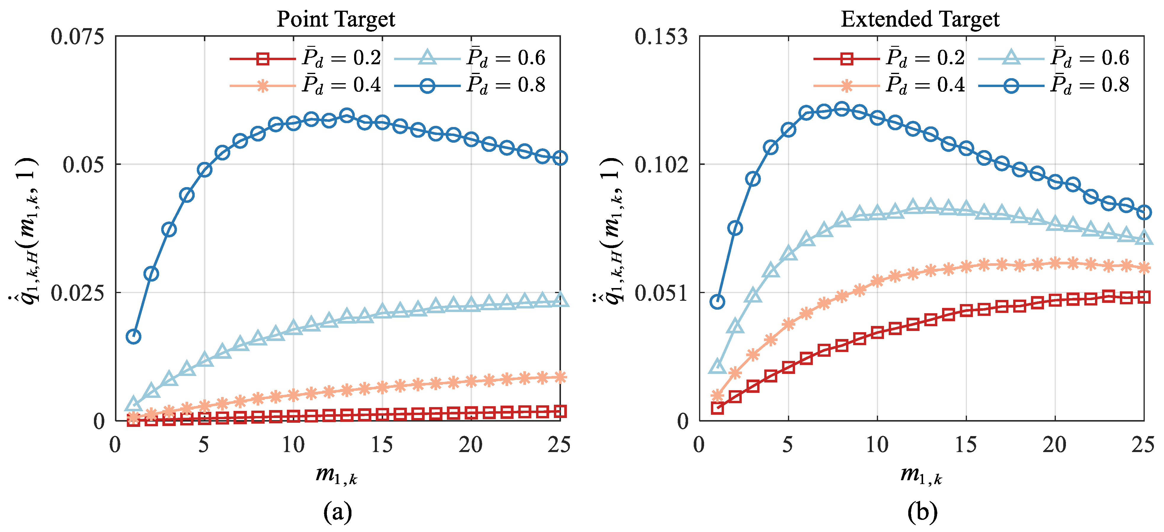
This paragraph’s detection probability P ¯ d still takes four values of 0.2 , 0.4 , 0.6 and 0.8 . Let λ ˜ 1 , k = 0.1 and λ ¯ 1 , k = 2 , then the point target‘s IRF q ^ ˙ 1 , k ( m 1 , k , 1 ) and the extended target’s SCIRF q ^ ¨ 1 , k ( m 1 , k , 1 ) under different detection probabilities are simulated, respectively. The results are shown in Figure 3.
As can be seen from Figure 3, on the one hand, when the detection probability P ¯ d and m 1 , k are given, the point target’s IRF q ^ ˙ 1 , k ( m 1 , k , 1 ) is smaller than the extended target’s SCIRF q ^ ¨ 1 , k ( m 1 , k , 1 ) . In fact, Appendix E shows that q ^ ˙ 1 , k ( m 1 , k , 1 ) is always greater than q ^ ¨ 1 , k ( m 1 , k , 1 ) . The reason for this phenomenon can be explained as follows. After making the difference between the two and arranging the Equation (A44), it is found that ϵ ¨ ( m 1 , k ) ϵ ˙ ( m 1 , k ) and ϵ ¨ ( m 1 , k ) + ϵ ˙ ( m 1 , k ) ϵ ¨ ( m 1 , k ) ϵ ˙ ( m 1 , k ) are the two factors that ultimately affect the positive and negative of the result. According to the discussion in Section 4.1.1, it can be known that ϵ ¨ ( m 1 , k ) ϵ ˙ ( m 1 , k ) > 0 . Then the property that ϵ ¨ ( m 1 , k ) and ϵ ˙ ( m 1 , k ) are both positive real numbers less than or equal to 1 guarantees ϵ ¨ ( m 1 , k ) + ϵ ˙ ( m 1 , k ) ϵ ¨ ( m 1 , k ) ϵ ˙ ( m 1 , k ) > 0 . From the perspective of physics, under the condition that the detection probability, clutter density, and measurement number are the same, because ϵ ¨ ( m 1 , k ) > ϵ ˙ ( m 1 , k ) , that is, the measurement in the sense of the extended target contains more useful information than the point target, then q ^ ¨ 1 , k ( m 1 , k , 1 ) will also contain more useful information than q ^ ˙ 1 , k ( m 1 , k , 1 ) , i.e., q ^ ¨ 1 , k ( m 1 , k , 1 ) > q ^ ˙ 1 , k ( m 1 , k , 1 )
On the other hand, the value of the extended target’s SCIRF q ^ ¨ 1 , k ( m 1 , k , 1 ) increases with the detection probability P ¯ d . Appendix D shows that the parameter C in Equation (A32) becomes large when P ¯ d is large, while the parameter A remains unchanged. In this case, the fraction C / ( A + C ) in Equation (A34) gradually increases, and the value of ϵ ¨ ( m 1 , k ) increases accordingly. The aforementioned change law means that the measurement in the sense of the extended target contains more helpful information than the point target, so the q ^ ¨ 1 , k ( m 1 , k , 1 ) also contains more useful information; that is, the q ^ ¨ 1 , k ( m 1 , k , 1 ) becomes larger.

4.1.3. Comparison among q ^ ¨ 1 , k ( m 1 , k , 1 ) with Different λ ˜ 1 , k

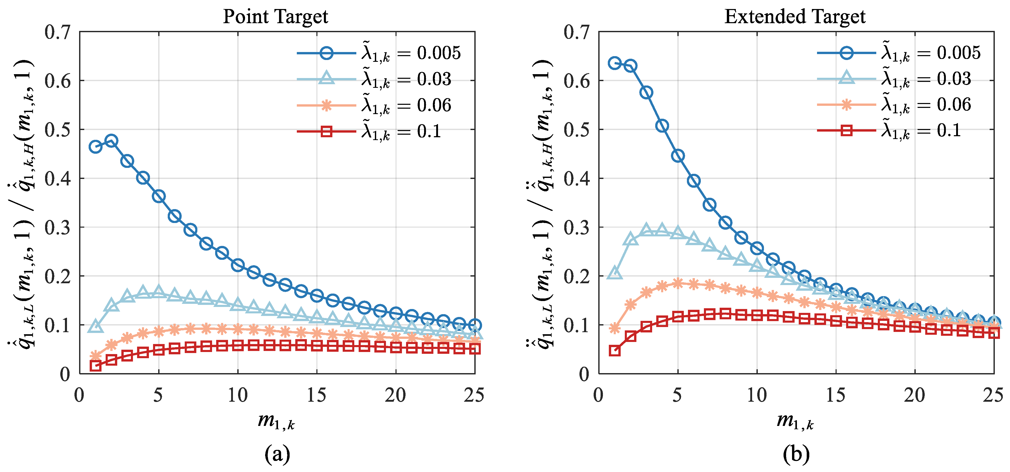
This paragraph’s clutter density λ ˜ 1 , k still takes four values of 0.1 , 0.06 , 0.03 , and 0.005 . Let λ ¯ 1 , k = 2 and P ¯ d = 0.8 , then the point target’s IRF q ^ ˙ 1 , k ( m 1 , k , 1 ) and the extended target’s SCIRF q ^ ¨ 1 , k ( m 1 , k , 1 ) under different λ ˜ 1 , k are simulated, respectively. The results are shown in Figure 4.
It can be seen from Figure 4 that, on the one hand, the point target’s IRF q ^ ˙ 1 , k ( m 1 , k , 1 ) is smaller than the extended target’s SCIRF q ^ ¨ 1 , k ( m 1 , k , 1 ) when the clutter density λ ˜ 1 , k and m 1 , k are given. Similar to the analysis of Figure 3, because ϵ ¨ ( m 1 , k ) contains more helpful information than ϵ ˙ ( m 1 , k ) , q ^ ¨ 1 , k ( m 1 , k , 1 ) can be made to contain more useful information than q ^ ˙ 1 , k ( m 1 , k , 1 ) .
On the other hand, the value of the extended target’s SCIRF q ^ ¨ 1 , k ( m 1 , k , 1 ) decreases with the increased clutter density. If ϵ ¨ ( m 1 , k ) is regarded as a continuous function of continuous variable λ ˜ 1 , k , ϵ ¨ ( m 1 , k ) ’s first derivative function to λ ˜ 1 , k can always be less than zero. In this case, when λ ˜ 1 , k becomes larger, the value of ϵ ¨ ( m 1 , k ) will decrease accordingly. The aforementioned change law means that the measurement in the sense of the extended target contains less helpful information, so the q ^ ¨ 1 , k ( m 1 , k , 1 ) also contains less useful information; that is, the q ^ ¨ 1 , k ( m 1 , k , 1 ) becomes smaller.

4.1.4. Global IRF and Global SCIRF under Different Detection Probability P ¯ d

In this section, Target 1 is taken as an example without loss of generality. The relationship among other parameters under the same clutter density and the relationship between different clutter densities and various parameters is quantitatively analyzed for the case of point target and extended target. On this basis, taking Case1 as an example, the power distribution of target positioning under different clutter densities is compared.
After calculating the point target IRF and the extended target SCIRF, this section further calculates the global IRF of the point target and the global SCIRF of the extended target. First, the strong clutter density λ ˜ 1 , k = 0.1 is given, then Table 2 shows the global SCIRF value of the extended target under different detection probabilities P ¯ d .
It can be seen from Table 4 that, on the one hand, the global SCIRF ϕ ¨ 1 , k , H of the extended target increases with the increase in the detection probability P ¯ d . This phenomenon can be explained as follows. Earlier paragraphs show that the q ^ ¨ 1 , k ( m 1 , k , 1 ) contains more useful information with the increase in detection probability, and its value will increase. According to the form of Equation (45), it can be seen that the parameter p T o m 1 , k and the p T o m 1 , k in P r n 1 , k | m 1 , k cancel out each other, while the rest does not contain the parameter P ¯ d . Therefore, the value of ϕ ¨ 1 , k , H will increase with the increase in q ^ ¨ 1 , k ( m 1 , k , 1 ) .
On the other hand, in calculating ϕ ¨ 1 , k , H , it is found that when m 1 , k and n 1 , k are both large, the q ^ ¨ 1 , k ( m 1 , k , 1 ) ’s value will be very large. However, the values of p T o m 1 , k and P r n 1 , k | m 1 , k at this time will also be very small. Therefore, according to Equation (45), it can be known that a reasonable value of ϕ ¨ 1 , k , H can be obtained after using p T o m 1 , k and P r n 1 , k | m 1 , k to “weighted average” q ^ ¨ 1 , k ( m 1 , k , 1 ) .
Secondly, low clutter density λ ˜ 1 , k = 0.005 is given, then Table 5 gives the global IRF ϕ ˙ 1 , k , L of the point target under different detection probabilities.
Table 5 shows that the point target’s global IRF ϕ ˙ 1 , k , L in the low clutter environment exhibits a similar variation rule to the extended target’s global SCIRF ϕ ¨ 1 , k , H in the strong clutter, which can also be explained in the same way as in Table 4. In addition, in this paper, the global SCIRF ϕ ˙ 1 , k , H of the point target in the strong clutter and the global IRF ϕ ¨ 1 , k , L of the extended target under the low clutter environment are also numerically simulated. The results show that the value of the point target’s global SCIRF ϕ ˙ 1 , k , H in the strong clutter is minimal, almost close to zero, which means that the measurement Z 1 , k is filled with much information about the clutter. In contrast, the value of the global IRF ϕ ¨ 1 , k , L of the extended target in the low clutter environment is huge, which means that the information from the target must be included in the measurement, which can be equivalent to the ideal situation. Since the point target’s global SCIRF ϕ ˙ 1 , k , H in strong clutter contains a small amount of information from the target, previous studies could not solve this complex problem. Based on the technology of improving the resolution of modern radar, this paper transitions the target from the traditional point target to the extended target so that the point target problem in strong clutter is transformed into the extended target problem in strong clutter. Then, the complicated problem can be solved.

4.2. Verification of Effectiveness of ERCC-PA Scheme

According to the analysis in Section 3.4, it can be seen that only the optimal total power 1 T p t opt corresponding to Case1 has both analytical and numerical solutions. Therefore, in this section, Case1 is used as an example to verify the effectiveness of the ERCC-PA scheme. On this basis, numerical simulation experiments are performed on Case2, Case3, and Case4. The confidence levels are set as 0.95, 0.85, and 0.7, respectively. Strong clutter density is λ ˜ 1 , k and the detection probability, P ¯ d = 0.8 .

4.2.1. Power Allocation of Case1: Swerling I and II

In traditional radar systems, power allocation does not require any prior knowledge, and the limited power resources are evenly allocated to multiple beams to illuminate multiple targets, which is the simplest case. Therefore, this paper takes the uniform power allocation as a benchmark and compares it with the ERCC-PA scheme.
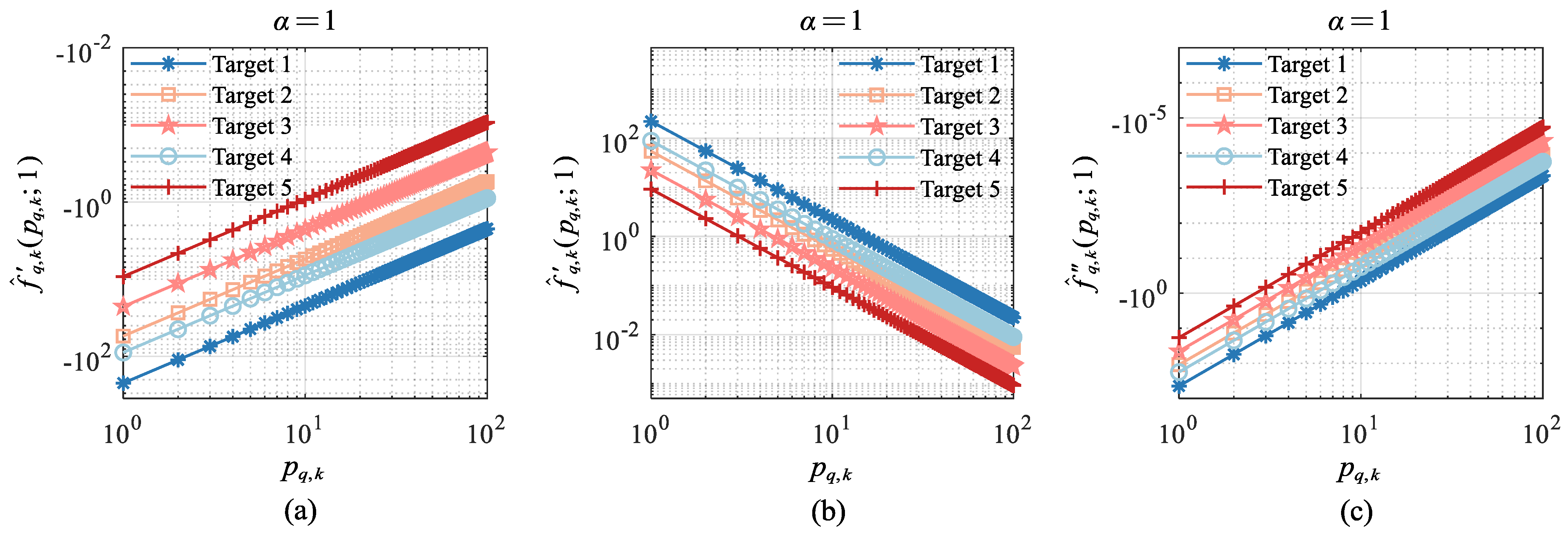
First, the image of the three functions f ^ q , k ( p q , k ; 1 ) , f ^ q , k ( p q , k ; 1 ) , and f ^ q , k ( p q , k ; 1 ) corresponding to α = 1 about the target q ( q = 1 , 2 , 3 , 4 , 5 ) in Case1 is given, as shown in Figure 5.
As can be seen from Figure 5, the monotonicity of f ^ q , k ( p q , k ; 1 ) , f ^ q , k ( p q , k ; 1 ) and f ^ q , k ( p q , k ; 1 ) are consistent with the theoretical analysis in Section 3.3. In particular, for equation f ^ q , k ( p q , k ; 1 ) = b / Q , which can be understood as a straight line y = b / Q parallel to the x-axis that intersects the function f ^ q , k ( p q , k ; 1 ) and has one and only one intersection with f ^ q , k ( p q , k ; 1 ) , i.e., a unique zero point. The same explanation can be for equation f ^ q , k ( p q , k ; 1 ) = ϑ . This property ensures that the above equation does not contain multiple zero points simultaneously. Therefore, an iterative dichotomy can directly approach this unique zero point, which verifies the correctness of the theoretical analysis.
Based on the above analysis, the optimal value of power p q , k can be obtained combined with the double dichotomy method in Algorithm 1. Figure 6 shows the results.
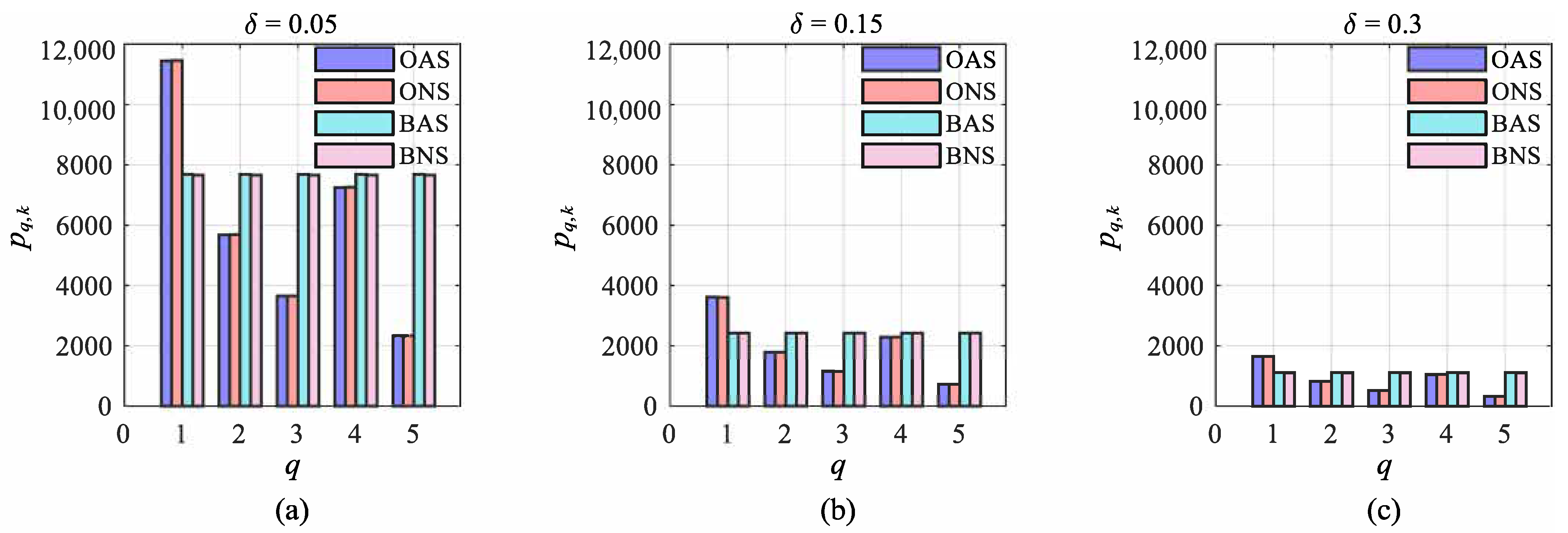
It can be seen from Figure 6 that, firstly, at different confidence levels, the optimal analytic solution (OAS) and the optimal numerical solution (ONS) of each target are almost the same. The benchmark’s analytical solution (BAS) and the benchmark’s numerical solution (BNS) for each target are also almost identical. Thus, the experimental results can verify the validity of the double dichotomy of the Γ -CCP model.
Secondly, the total transmitted power consumed by SM-DAR decreases with the decrease in confidence level 1 δ . From the perspective of mathematics, according to Equation (63), it can be seen that the transmission power of each target is an increasing function of parameter b. Therefore, when 1 δ decreases, b decreases. Then, the transmission power of each target decreases, and thus, the total transmission power of SM-DAR decreases. From the physical point of view, first, consider a particular case of Problem (55): the trace of PCRLB corresponding to each target does not exceed the given threshold P r { F p 1 , k , ξ 1 , k η 1 , F p 2 , k , ξ 2 , k η 2 , , F p Q , k , ξ Q , k η Q } = 1 with probability 1. In this case, the transmitted power of SM-DAR will be reduced due to some values in the RCS’s domain so that its detection distance is relatively close. If the detection distance has exceeded the given threshold, the SM-DAR’s transmitted power must be increased to make the trace of the target corresponding to the PCRLB can not exceed the given threshold. If the confidence level is reduced, the requirement that the trace of PCRLB corresponding to each target does not exceed the given threshold will be relatively loose and easy to achieve. In other words, the reduction of confidence level allows the situation that the trace of PCRLB corresponding to a certain target to exceed the given threshold with a certain probability can occur. Therefore, when faced with a situation where the detection distance of SM-DAR exceeds the threshold due to the value of RCS, the low confidence level has allowed this kind of situation to occur, so it is no longer necessary to increase the transmitted power of SM-DAR to ensure that the detection distance “must” not exceed the given threshold. Therefore, the reduction of confidence level will reduce the total transmit power consumed by SM-DAR accordingly.
Thirdly, for Target 1 and Target 2 of RCS with the same distribution parameters, the former consumes more power. According to the simulation experiment, it is found that the longer the distance of the target will increase the value of ς q , k . According to Equation (63), the power consumption of the target increases with the increase in ς q , k . Therefore, the power consumption of Target 1 is greater than that of Target 2. From a practical point of view, since the distance of Target 1 is longer, in the same case, it is necessary to consume higher power than Target 2 to make the detection distance of SM-DAR exceed Target 2 and reach the threshold of Target 1. Similarly, Target 4 consumes more power than Target 5.
Fourthly, for Target 3 and Target 5 with the same distance, the former consumes more power. According to Equation (63), it can be seen that the power consumption of the target is a decreasing function of the mean value h ¯ q , k of the target’s RCS. According to the relationship of h ¯ 3 , k < h ¯ 5 , k , Target 3 consumes more power than Target 5. From a practical perspective, for a target with a smaller RCS’s mean value, the value within its RCS’s domain will be taken near its mean value with a greater probability. Therefore, if the detection distance of Target 3 is always smaller than that of Target 5, the situation that the given threshold is exceeded will occur. To make the localization effect of Target 3 equivalent to that of Target 5, it is necessary to put a higher value on SM-DAR when locating Target 3, to achieve.

4.2.2. Power Allocation of Case2: Swerling III and IV, Case3 and Case4

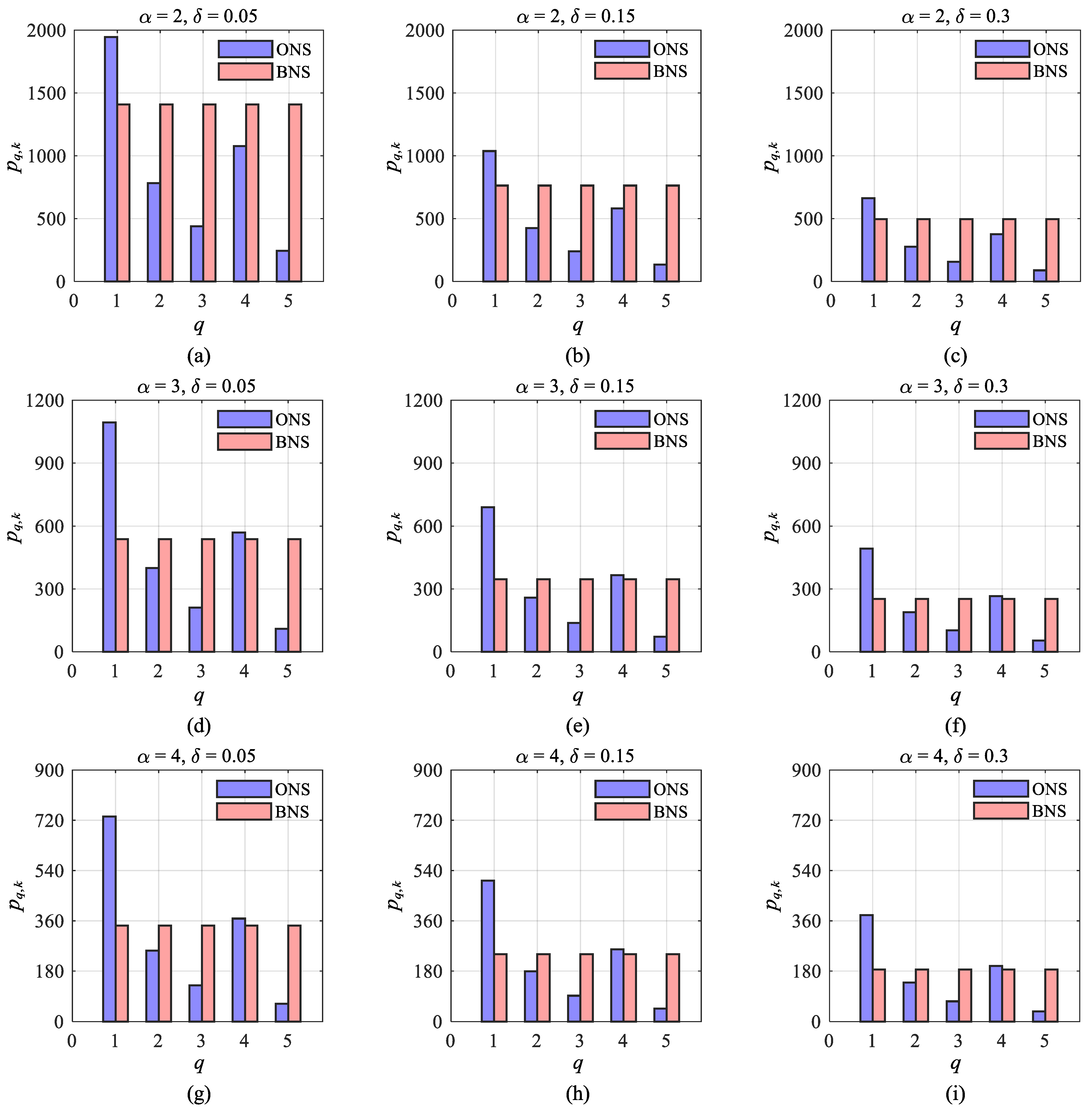
According to the analysis in Section 3.4.2, it can be seen that Case2, Case3, and Case4 do not have analytical solutions for power allocation due to the limitation of the absence of analytical solutions and general solutions for transcendental equations and higher-order equations. Therefore, this section will use Algorithm 1 to simulate the optimal power allocation of Case2, Case3, and Case4, as shown in Figure 7.
Through the horizontal comparison, it is found that the power allocation of Case2, Case3, and Case4 in Figure 7 shows a similar law to that of Case1. For example, for each of Case2, Case3, and Case4, the total transmitted power consumed by the SM-DAR decreases as the confidence level decreases. For Target 1 and Target 2 with the same RCS mean value, Target 1 with greater distance consumes more power than Target 2.
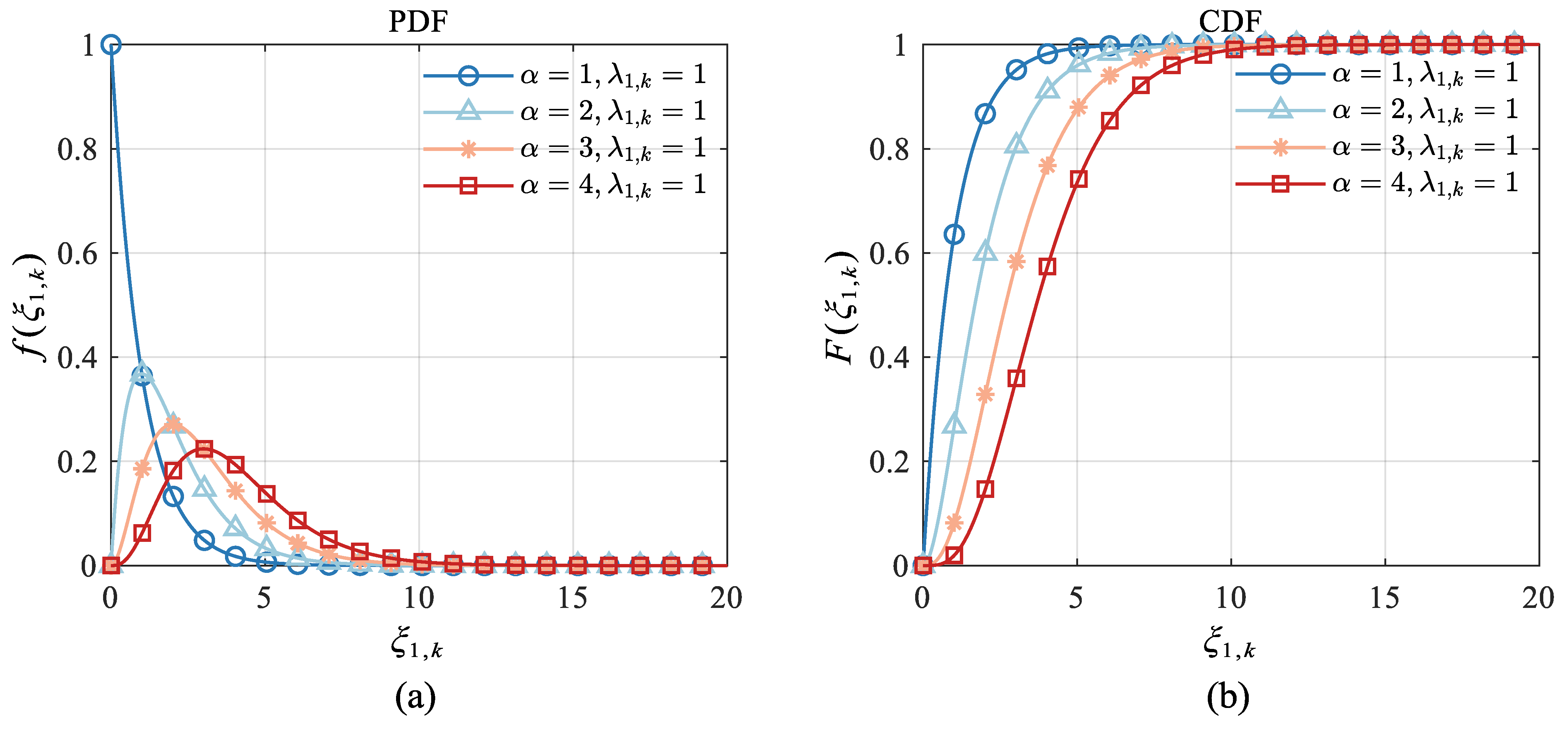
Through longitudinal comparison, still taking Target 1 as an example, it can be found that under the same confidence level, the power consumption of Target 1 decreases with the increase in the shape parameter. Certain properties of the Gamma distribution determine this phenomenon. Figure 8 shows the PDF and CDF of the Gamma distributions of different shape parameters in Case1, Case2, Case3, and Case4.
It can be seen from Figure 8 that the larger the value of α , the slower the rate at which the corresponding Γ distribution’s CDF tends to 1. This rule shows that random variable Ξ 1 , k with a larger α value is more likely to take the larger value in its domain than Ξ 1 , k with a smaller α value. Take the two curves corresponding to α = 1 and α = 4 in Figure 8b as an example. When ξ 1 , k = 5 , the cumulative probability values of the two curves here are F α = 1 ( 5 ) = 0.9933 and F α = 4 ( 5 ) = 0.7350 , respectively. Therefore, when α = 1 , the probability that Ξ 1 , k can obtain the range ( 5 , + ) is much less than when α = 4 , that is, P r α = 1 ( ξ 1 , k > 5 ) = 1 F α = 1 ( 5 ) = 0.0067 < 0.2650 = 1 F α = 4 ( 5 ) = P r α = 4 ( ξ 1 , k > 5 ) . Based on the above analysis, it can be seen that the probability of RCS of Target 1 taking the larger value in its domain will increase with the increase in α = 1 , i.e., in actual detection, RCS with a larger α = 1 value will take the larger value in its definition domain more times than RCS with smaller α = 1 value. Considering the negative correlation between RCS and target power consumption, it can be seen that the power consumption of Target 1 will decrease with the increase in shape parameter α = 1 . This conclusion also applies to target q ( q = 2 , 3 , 4 , 5 ) .
Since the power consumption of each target decreases with the increase in the shape parameter α , the sum of the power consumption of all targets, that is, the total power consumption 1 T p k opt of the ERCC-PA scheme also decreases with the increase in the shape parameter α . Similarly, 1 T p k opt also decreases as the confidence level 1 δ decreases. Table 6 quantitatively presents the variation law of the total power consumption 1 T p k opt of the ERCC-PA scheme with the shape parameter α and the confidence level 1 δ .
Table 7 further presents the power saving rates of Case1, Case2, Case3, and Case4 compared to the benchmark at different confidence levels.
Combining the four cases of Case1, Case2, Case3, and Case4, it can be seen that under the condition that the multi-target joint PCRLB probability is greater than or equal to the preset confidence level 1 δ , the SM-DAR needs to allocate its power resources to different beams reasonably. Specifically, for multiple targets with the same localization accuracy threshold, the ERCC-PA scheme tends to the following two situations:
  • When the target number of RCSs with the same expectation ξ ¯ q , k = α / λ q , k is Q > 1 , more power resources can be allocated to the farther targets (such as the allocation results of Target 1 and Target 4);
  • Under the condition that the number of targets with the same distance is Q > 1 , more power resources are allocated to the target with a smaller average RCS (such as the allocation results of Target 3 and Target 5).

4.3. Robustness of ERCC-PA Scheme

When the previous research regards RCS as a deterministic variable, the corresponding power allocation scheme “does not allow” the situation that the PCRLB of each target exceeds the respective preset thresholds, i.e.,
P r F p 1 , k , ξ 1 , k η 1 , k , F p 2 , k , ξ 2 , k η 2 , k , , F p Q , k , ξ Q , k η Q , k = 1 .
However, after the RCS is further regarded as a random variable, the corresponding RCC-PA scheme [31], and the ERCC-PA scheme proposed in this paper will “allow” each target’s PCRLB to exceed their respective preset thresholds with a certain probability occurs, that is,
P r F p 1 , k , ξ 1 , k η 1 , k , F p 2 , k , ξ 2 , k η 2 , k , , F p Q , k , ξ Q , k η Q , k 1 δ .
which is more in line with the actual situation.
In terms of the real scene, it is often difficult to predict the actual RCS value of the target q at the current time k in real time and accurately. The practice for overcoming this difficulty is usually to arithmetically average the RCS values at all times in a certain period [ s , k 1 ] before time k. According to the strong law of large numbers, the arithmetic means ξ ¯ q , k can be taken as the RCS mean at the current time k to achieve the optimal power allocation of each target. If the actual value of RCS fluctuates wildly around the mean value ξ ¯ q , k and the optimal power p k opt does not change, p k opt is not sensitive to such fluctuations. This property is very consistent with the ideas of the methods currently used in practice. In other words, the optimal power allocation results must be robust to RCS fluctuations within a certain range. Therefore, this section can take the optimal power allocation p k opt of all cases in Section 4.2 as a known condition, generate N M C random numbers of the corresponding RCS in each case, and calculate and count the ratio 1 δ opt of the number of random numbers satisfying the condition F ( p q , k opt , ξ q , k ) η q , k ( q = 1 , 2 , , Q ) to N M C . If 1 δ opt and 1 δ are very close, the ERCC-PA scheme is robust. On this basis, the robustness of the ERCC-PA scheme can be accurately measured quantitatively.

4.3.1. Verification of Robustness of the ERCC-PA Scheme

The above analysis shows that if not all the targets q ( q = 1 , 2 , , Q ) satisfy the conditions in Equation (50), the optimal power needs to be changed to make F ( p q , k opt , ξ q , k ) η q , k ( q = 1 , 2 , , Q ) all established. If the optimal power remains unchanged, some inequalities in F ( p q , k opt , ξ q , k ) η q , k ( q = 1 , 2 , , Q ) must no longer hold.
At this time, the number of RCS random numbers that cannot make F ( p q , k opt , ξ q , k ) η q , k ( q = 1 , 2 , , Q ) all true can be counted through Monte Carlo trials. The significance level under optimal power p k opt is denoted as [31]
δ opt = 1 N M C i = 1 N M C I 2 max q F p q , k opt , ξ q , k ( i ) η q , k .
where ξ q , k ( i ) is the real RCS’s value of Target q in the ith test. The definition of the indicative function
I 2 a = 1 , a > 0 , 0 , a 0 .
After the Monte Carlo simulation test is completed, the calculation is performed according to Equation (68), and Table 8 can be obtained.
It can be seen from Table 8 that the 1 δ opt under the optimal power p k opt in the ERCC-PA scheme is almost the same as the pre-given confidence level 1 δ , indicating the ERCC-PA scheme has robustness.

4.3.2. Metrics of Robustness of the ERCC-PA Scheme

To further measure the robustness of the ERCC-PA scheme, the following formula can be obtained according to the definition of relative error.
ρ = δ opt δ δ × 100 % .
where ρ is also called the metrics of the ERCC-PA scheme’s robustness.
According to Equation (70), the closer ρ is to zero, the stronger the robustness of the ERCC-PA scheme is. The reason for this phenomenon can be explained as follows. When ρ is close to zero, δ opt is infinitely close to δ , which means that the target’s optimal power allocation remains unchanged under RCS fluctuation. This event indeed occurs with a probability greater than or equal to 1 δ .
Table 9 further gives the measurement of the ERCC-PA scheme’s robustness under different confidence levels 1 δ = 0.95 , 0.85 , 0.70 .
It can be seen from Table 9 that under different shape parameters α and different confidence levels 1 δ , the robustness metrics ρ is small, indicating that the ERCC-PA scheme has strong robustness to the fluctuation of target’s RCS.

5. Conclusions

Relying on modern radar technology, high-resolution SM-DAR, extended target, and the uncertainty of RCS are used in strong clutter in this paper. Combined with the RCC-PA scheme, the ERCC-PA scheme is constructed to solve the multi-target localization power allocation problem that is more in line with the current radar detection environment. In this scheme, the high-resolution SM-DAR can endow the target with multi-measurement characteristics and make it have a better global SCIRF to achieve a reasonable allocation for the power of multi-target localization in strong clutter is verified for the first time. At the same time, the proposed Gamma target RCS model extends the generality of the RCC-PA scheme to a certain extent, and the relationship between the shape parameters of the Gamma distribution and the power allocation of multi-target localization is also reasonably explained in the mathematical and physical level. On this basis, the correctness of the theoretical analysis is verified by the extended numerical algorithm, and the robustness of the ERCC-PA scheme is demonstrated.
This paper initially examines how factors such as strong clutter, high-resolution SM-DAR, extended target, and RCS uncertainty affect the power allocation for target localization. However, the above factors still need further exploration to make the ERCC-PA scheme more general. For example, the acquisition of clutter expressions in the multi-target multi-sensor situation, the case where the RCS distribution type belongs to other distribution families, and how to successfully apply the ERCC-PA scheme to practical engineering problems. Deep neural networks have been widely employed in natural language processing [39], Learning Knowledge Graph Embedding With Heterogeneous Relation Attention Networks, and computer vision [40]. In the future, we will examine the deep learning technique [41] for the power allocation of multiple target localization.

Author Contributions

Conceptualization, L.W. and D.Z.; Methodology, C.X.; Software, C.X.; Validation, C.X., L.W. and D.Z.; Formal analysis, C.X.; Resources, D.Z.; Writing–original draft, C.X.; Writing–review & editing, C.X.; Supervision, D.Z.; Project administration, L.W. and D.Z. All authors have read and agreed to the published version of the manuscript.

Funding

This work is supported by the National Key Research and Development Program of China with Grant No. 2017YFB0502700, the National Natural Science Foundation of China with Grant No. 61871217, the Aviation Science Foundation with Grant No. 20182052011 and the Postgraduate Research and Practice Innovation Program of Jiangsu Province with the Grant No. KYCX18_0291, the Fundamental Research Funds for Central Universities under Grant NZ2020007, and the Fundamental Research Funds for Central Universities under Grant NG2020001.

Data Availability Statement

Not applicable.

Conflicts of Interest

The authors declare no conflict of interest.

Appendix A. Nomenclature

The naming conventions of the main symbols in the text are shown in Table A1.
Table A1. Nomenclature.
ParameterDefinition
P r · Probability value
F · Cumulative Distribution Function (CDF)
f · Probability Density Function for continuous random variables (PDF)
p · Probability Mass Function for discrete random variables (PMF)
ζ q , k State vector of target q at time k
n z Dimension of ζ q , k
h q , k ζ q , k Observation vector of ζ q , k at time k
h q , k ζ q , k j The jth index in h q , k ζ q , k
σ j Error standard deviation of h q , k ζ q , k j
m q , k Number of all measurements within the threshold of target q at time k
n q , k Number of real targets measured within the threshold of target q at time k
r q , k Number of false alarms measured within the threshold of target q at time k
Ψ Number of combinations given m q , k and n q , k , i.e., Ψ = C m q , k n q , k
Z q , k Random measurement vector group, i.e., Z q , k = Z q , k i i = 1 , , m q , k
Z q , k i The ith measurement
Z ¯ q , k i The ith measurement is the real target
Z ˜ q , k i The ith measurement is false alarm
n x Dimensions of h q , k ζ q , k , Z q , k i , Z ¯ q , k i and Z ˜ q , k i
z q , k Values of all measurements, i.e F z q , k = P r Z q , k z q , k
z q , k i Value of Z q , k i , i.e., F z q , k i = P r ( Z q , k i z q , k i )
z ¯ q , k i Value of Z ¯ q , k i , i.e., F z ¯ q , k i = P r ( Z ¯ q , k i z ¯ q , k i )
z ˜ q , k i Value of Z ˜ q , k i , i.e., F z ˜ q , k i = P r ( Z ˜ q , k i z ˜ q , k i )
Z q , k i j The jth component of Z q , k i , i.e., one-dimensional random variable
Z ¯ q , k i j The jth component of Z ¯ q , k i , i.e., one-dimensional random variable
Z ˜ q , k i j The jth component of Z ˜ q , k i , i.e., one-dimensional random variable
z q , k i j Value of Z q , k i j , i.e., F z q , k i j = P r ( Z q , k i j z q , k i j )
z ¯ q , k i j Value of Z ¯ q , k i j , i.e., F z ¯ q , k i j = P r ( Z ¯ q , k i j z ¯ q , k i j )
z ˜ q , k i j Value of Z ˜ q , k i j , i.e., F z ˜ q , k i j = P r ( Z ˜ q , k i j z ˜ q , k i j )
[ Z q , k ] Ψ k i The ith measurement in the kth combination when the combination number is Ψ
[ Z ¯ q , k ] Ψ k i In the kth combination with combination number Ψ , the ith measurement is the real target
[ Z ˜ q , k ] Ψ k i In the kth combination with combination number Ψ , the ith measurement is the false alarm
[ z q , k ] Ψ k i Value of [ Z q , k ] Ψ k i , i.e., F ( [ z q , k ] Ψ k i ) = P r ( [ Z q , k ] Ψ k i [ z q , k ] Ψ k i )
[ z ¯ q , k ] Ψ k i Value of [ Z ¯ q , k ] Ψ k i , i.e., F ( [ z ¯ q , k ] Ψ k i ) = P r ( [ Z ¯ q , k ] Ψ k i [ z ¯ q , k ] Ψ k i )
[ z ˜ q , k ] Ψ k i Value of [ Z ˜ q , k ] Ψ k i , i.e., F ( [ z ˜ q , k ] Ψ k i ) = P r ( [ Z ˜ q , k ] Ψ k i [ z ˜ q , k ] Ψ k i )
ϵ ˙ ( m q , k ) Probability that measurement Z q , k contains point target q’s measurement.
ϵ ¨ ( m q , k ) Probability that measurement Z q , k contains extended target q’s measurement.
q ^ ˙ ( m q , k , n q , k ) IRF of point target q
q ^ ¨ ( m q , k , n q , k ) IRF of extended target q.
ϕ ˙ q , k Global IRF of point target q.
ϕ ¨ q , k Global IRF of extended target q.

Appendix B. Proof of Global SCIRF for Extended Targets

Proof. 
According to the property that the order of summation and integration can be exchanged, Equation (34) can be simplified as
Q ^ q , k m q , k , n q , k = ϵ m q , k 2 Ψ 2 V q , k 2 r q , k · 1 | 2 π R q , k | n q , k l 1 = 1 Ψ l 2 = 1 Ψ z ¯ q , k 1 A z ¯ q , k n q , k A · Combination of real targets z ˜ q , k 1 A z ˜ q , k r q , k A Combination of false alarms R q , k 1 φ z ¯ q , k Ψ l 1 i φ z ¯ q , k Ψ l 2 i T f z q , k | ζ q , k , m q , k , n q , k d A .
To further simplify Equation (A1), the following assumptions can be made [7].
  • Assumption A1. To reduce the amount of calculation, the measurement is limited to a certain threshold as below,
    | [ Z ¯ q , k ] Ψ l i j h q , k ζ q , k j | < g σ j , i = 1 , 2 , , m q , k , j = 1 , 2 , , n x , l = 1 , 2 , , Ψ .
    where  [ Z ¯ q , k ] Ψ ( l ) i j  denotes the jth component of the measured value  [ Z ¯ q , k ] Ψ ( l ) i h q , k ( ζ q , k j )  represents the jth component of  h q , k ( ζ q , k ) , and  σ j  is the jth component’s error standard deviation of the measured vector.
  • Assumption A2. The dimensions of the measured values are orthogonal to each other, then A can be represented by a hypercube
    A = [ g σ 1 , g σ 1 ] × [ g σ 2 , g σ 2 ] . . . × [ g σ n x , g σ n x ] .
    and the hypercube’s volume is
    V q , k = 2 g n x i = 1 n x σ i = 2 g n x | R q , k | .
and since Equation (A1) is independent of ζ q , k and when i j is satisfied, the integrand is odd symmetric and the integral region is symmetric. Let
z ¯ q , k Ψ l i = z q , k Ψ l i h q , k ζ q , k .
and combined with the above assumptions, Equation (A1) can be further written as
Q ^ q , k m q , k , n q , k = Π m q , k , n q , k Ψ 2 V q , k 2 r q , k · ϵ m q , k 2 2 π R q , k n q , k g σ 1 g σ 1 g σ n x g σ n x n q , k × n x g σ 1 g σ 1 g σ n x g σ n x r q , k × n x R q , k 1 z ¯ q , k 1 z ¯ q , k 1 T exp n q , k z ¯ q , k 1 R q , k 1 z ¯ q , k 1 T / 1 ϵ m q , k ( V q , k ) m q , k + ϵ m q , k Ψ ( V q , k ) r q , k · 1 | 2 π R q , k | n q , k k = 1 Ψ exp i = 1 n q , k 1 2 z ¯ q , k Ψ l i T R q , k 1 z ¯ q , k Ψ l i d z ¯ q , k 1 d z ¯ q , k n q , k d z ˜ q , k 1 d z ˜ q , k r q , k
In Equation (A6), z q , k Ψ l i = z q , k Ψ l i h q , k ζ q , k , σ j ( j = 1 , 2 , , n x ) represents the error standard deviation of the jth component of the measurement vector, and the even symmetric term coefficient Π ( m q , k , n q , k ) has two different forms according to the parity of m q , k .
When m q , k = 2 n 1 , n N + , Π ( m q , k , n q , k ) has the following form
Π m q , k , n q , k = h = 0 n q , k n q , k h C m q , k n q , k h C r q , k + h h C r q , k h , n q , k m q , k 1 / 2 , h = 0 m q , k 1 / 2 l 1 * + 1 n q , k h C m q , k n q , k h C r q , k + h h C r q , k h , n q , k = m q , k 1 / 2 + l 1 * , n q , k , n q , k = m q , k . l 1 * = 1 , 2 , , m q , k 1 / 2 .
When m q , k = 2 n , n N + , Π ( m q , k , n q , k ) has the following form
Π m q , k , n q , k = h = 0 n q , k n q , k h C m q , k n q , k h C r q , k + h h C r q , k h , n q , k m q , k / 2 , h = 0 m q , k / 2 l 2 * n q , k h C m q , k n q , k h C r q , k + h h C r q , k h , n q , k = m q , k 1 / 2 + l 2 * , n q , k , n q , k = m q , k . l 2 * = 1 , 2 , , m q , k / 2 1 .
On this basis, the measurement vector [ z ¯ q , k ] Ψ l i can be specifically expressed as
z ¯ q , k Ψ l i = z ¯ q , k Ψ l i 1 , z ¯ q , k Ψ l i 2 , , z ¯ q , k Ψ l i n x T .
then Equation (A6) can be simplified
Q ^ q , k m q , k , n q , k a b = Π m q , k , n q , k Ψ 2 V q , k 2 r q , k · ϵ m q , k 2 2 π R q , k n q , k g σ 1 g σ 1 g σ n x g σ n x n q , k × n x g σ 1 g σ 1 g σ n x g σ n x r q , k × n x z ¯ q , k 1 a z ¯ q , k 1 b σ a σ b exp n q , k i = 1 n x z ¯ q , k Ψ l 1 i σ i 2 / { 1 ϵ m q , k ( V q , k ) m q , k + ϵ m q , k Ψ ( V q , k ) r q , k · 1 2 π R q , k n q , k k = 1 Ψ exp { r = 1 n q , k 1 2 i = 1 n x z ¯ q , k Ψ l r i σ i } } d z ¯ q , k 1 d z ¯ q , k n q , k d z ˜ q , k 1 d z ˜ q , k r q , k
where [ Q ^ q , k ( m q , k , n q , k ) ] a b represents the element in the ath row and bth column of matrix Q ^ q , k ( m q , k , n q , k ) .
When a b is satisfied, [ Q ^ q , k ( m q , k , n q , k ) ] a b = 0 holds, otherwise, [ Q ^ q , k ( m q , k , n q , k ) ] a a 0 . Then,
Q ^ q , k ( m q , k , n q , k ) 11 = Q ^ q , k ( m q , k , n q , k ) 22 = = Q ^ q , k ( m q , k , n q , k ) n x n x .
From Equation (A11), it can be seen that [ Q ^ q , k ( m q , k , n q , k ) ] a a only needs to be further simplified. Substitute the following transformation
z q , k r i = z q , k r i σ i , r = 1 , 2 , , m q , k , i = 1 , 2 , n x .
into Equation (A10), the final form of [ Q ^ q , k ( m q , k , n q , k ) ] a a is
Q ^ q , k m q , k , n q , k a a = Π m q , k , n q , k Ψ 2 ( V q , k ) 2 r q , k · ϵ m q , k 2 R q , k 0.5 m q , k n q , k 2 π n x n q , k g g g g n q , k × n x g g g g r q , k × n x { z ¯ q , k 1 a 2 exp n q , k i = 1 n x z ¯ q , k 1 i 2 } / { 1 ϵ m q , k ( V q , k ) m q , k + 1 Ψ · ϵ m q , k ( V q , k ) r q , k | 2 π R q , k | n q , k k = 1 Ψ exp { r = 1 n q , k 1 2 i = 1 n x z ¯ q , k Ψ l r i } d z ¯ q , k 1 d z ¯ q , k n q , k d z ˜ q , k 1 d z ˜ q , k r q , k
where a = 1 , . . . , n x .
Let q ^ q , k ( m q , k , n q , k ) denote SCIRF, then the relationship between q ^ q , k ( m q , k , n q , k ) and
[ Q ^ q , k ( m q , k , n q , k ) ] a a is
q ^ q , k ( m q , k , n q , k ) = [ Q ^ q , k m q , k , n q , k ] a a , a = 1 , 2 , , n x .
Therefore, the following equation holds
Q ^ q , k m q , k , n q , k = q ^ q , k ( m q , k , n q , k ) × I n x .
where I n x is an n x -order identity matrix, and q ^ q , k ( m q , k , n q , k ) is not related to ζ q , k , then
J ( k : m q , k : n q , k ) = q ^ q , k ( m q , k , n q , k ) E ζ q , k [ ( H q , k ) T R q , k 1 H q , k ] .
Equation (A16) is the simplest form of CFIM. On this basis, FIM J ( ζ q , k ) can be given by the following formula
J ( ζ q , k ) = E m q , k , n q , k J k , m q , k , n q , k = E ζ q , k [ ( H q , k ) T R q , k 1 H q , k ] · E m q , k , n q , k [ q ^ q , k ( m q , k , n q , k ) ] = E ζ q , k [ ( H q , k ) T R q , k 1 H q , k ] m q , k = 1 p T o ( m q , k ) n q , k = 1 m q , k [ P r ( n q , k | m q , k ) q ^ q , k ( m q , k , n q , k ) ] .
where
P r n q , k | m q , k = p F a r q , k p T r ( n q , k ) p T o ( m q , k ) = 1 p T o ( m q , k ) · ( λ ˜ q , k V q , k ) r q , k e λ ˜ q , k V q , k r q , k ! · ( λ ¯ q , k ) n q , k e λ ¯ q , k n q , k ! .
Let
ϕ q , k = m q , k = 1 p T o ( m q , k ) n q , k = 1 m q , k [ P r ( n q , k | m q , k ) q ^ q , k ( m q , k , n q , k ) ] .
then Equation (A17) can be simplified as
J ( ζ q , k ) = ϕ q , k · E ζ q , k [ ( H q , k ) T R q , k 1 H q , k ] .
Equation (A20) is the simplest form of FIM. Moreover, by synthesizing Equations (A19) and (A20), it can be seen that ϕ q , k is the global SCIRF. □

Appendix C. Proof of the Convexity for the Optimization Problem

Proof. 
Based on the equivalent transformation in Section 3.4.1, the convexity of the Γ -CCP model can be discussed through Problem (59). Since Problem (59) is linear except for the first constraint, it is only necessary to prove the convexity of the first constraint. For the values of different shape parameters α , the first constraint function can be uniformly written as
f u n ( p k ) 0
where
f u n ( p k ) = q = 1 Q ln 1 Γ α Γ α , λ q , k ς q , k p q , k b
According to the relevant theory of convex optimization [31] when the Hessian matrix of f u n ( p k ) is negative define, it is concave, and it can be proved that Equation (A21) is a convex constraint. Therefore, first, calculate the first derivative of f u n ( p k ) for p k as follows:
P f u n ( p k ) = [ f ^ 1 , k ( p 1 , k ) , , f ^ Q , k ( p q , k ) ] T
where
f ^ q , k p q , k = 1 p q , k λ q , k ς q , k p q , k α 1 Γ α , λ q , k ς q , k p q , k exp λ q , k ς q , k p q , k .
Continue to calculate the second-order partial derivative of Equation (A24), and the Hessian matrix of function f u n ( p k ) can be obtained as follows:
p k p k f u n ( p k ) = d i a g { f ^ 1 , k ( p 1 , k ) , , f ^ Q , k ( p q , k ) }
where the symbol p k p k = p k p k T represents the second-order partial derivative operator
f ^ q , k p q , k = 1 p q , k 2 λ q , k ς q , k p q , k α 1 Γ 2 α , λ q , k ς q , k p q , k exp λ q , k ς q , k p q , k · λ q , k ς q , k p q , k α + 1 Γ α , λ q , k ς q , k p q , k λ q , k ς q , k p q , k α exp λ q , k ς q , k p q , k .
where Γ α , · is the upper incomplete Gamma function of parameter α . When α is a positive integer, the explicit expression of Γ α , · is
Γ α , λ q , k ς q , k p q , k = exp λ q , k ς q , k p q , k λ q , k ς q , k p q , k α 1 + i = 1 α 1 α i + i = 2 α 1 λ q , k ς q , k p q , k α i j = 1 i 1 α j .
From the definition of PCRLB [12], the domain of function f ^ q , k p q , k is 0 , + , p q , k > 0 , λ q , k > 0 and ς q , k > 0 .
In this case, Equation (A27) can be substituted into Equations (A24) and (A26) to see f ^ q , k ( p q , k ) > 0 and f ^ q , k ( p q , k ) < 0 . Therefore, the Γ -CCP model in this paper has the following properties:
(1)
For all shape parameters α , f ^ q , k ( p q , k ) is a monotone increasing function of p q , k ;
(2)
For all shape parameters α , f ^ q , k ( p q , k ) is a monotone decreasing function of p q , k ;
(3)
For all shape parameters α , the Hessian matrix p k p k f u n ( p k ) is negative definite, which means that the constraint function f u n ( p k ) is concave.
Based on the above analysis, it can be seen that the first constraint f u n ( p k ) 0 in Problem (55) is convex, so the Γ -CCP model is a convex optimization problem. □

Appendix D. Size Relationship between ϵ ˙ m 1 , k and ϵ ¨ m 1 , k When λ ¯ 1 , K = 1

According to Ref. [12], it can be seen that the parameters p ˙ T o m 1 , k and ϵ ˙ m 1 , k corresponding to the point target q = 1 have the following forms
p ˙ T o m 1 , k = 1 P ¯ d λ ˜ 1 , k V 1 , k m 1 , k m 1 , k ! e λ ˜ 1 , k V 1 , k + P ¯ d λ ˜ 1 , k V 1 , k m 1 , k 1 m 1 , k 1 ! e λ ˜ 1 , k V 1 , k .
ϵ ˙ m 1 , k = P ¯ d p ˙ T o m 1 , k · λ ˜ 1 , k V 1 , k m 1 , k 1 m 1 , k 1 ! e λ ˜ 1 , k V 1 , k .
Substituting Equations (A28) and (26) into Equations (A29) and (32), respectively, then
ϵ ˙ m 1 , k = P ¯ d λ ˜ 1 , k V 1 , k m 1 , k 1 m 1 , k 1 ! / 1 P ¯ d λ ˜ 1 , k V 1 , k m 1 , k m 1 , k ! + P ¯ d λ ˜ 1 , k V 1 , k m 1 , k 1 m 1 , k 1 ! .
ϵ ¨ m 1 , k = P ¯ d 1 + λ ˜ 1 , k V 1 , k m 1 , k λ ˜ 1 , k V 1 , k m 1 , k m 1 , k ! / 1 P ¯ d λ ˜ 1 , k V 1 , k m 1 , k m 1 , k ! + P ¯ d 1 + λ ˜ 1 , k V 1 , k m 1 , k λ ˜ 1 , k V 1 , k m 1 , k m 1 , k ! .
If let
A = 1 P ¯ d λ ˜ 1 , k V 1 , k m 1 , k m 1 , k ! , B = P ¯ d λ ˜ 1 , k V 1 , k m 1 , k 1 m 1 , k 1 ! , C = P ¯ d 1 + λ ˜ 1 , k V 1 , k m 1 , k λ ˜ 1 , k V 1 , k m 1 , k m 1 , k ! .
then Equations (A30) and (A31) can be rewritten as
ϵ ˙ m 1 , k = B A + B ,
and
ϵ ¨ m 1 , k = C A + C ,
respectively. Subtracting Equations (A34) and (A33), the following equation can be obtained
ϵ ¨ m 1 , k ϵ ˙ m 1 , k = A A + B A + C C B .
Since A , A + B and A + C are all greater than zero, only the positive and negative of C B need to be discussed. By appropriately processing the variable C, the following relational expression can be obtained
C = P ¯ d 1 + λ ˜ 1 , k V 1 , k m 1 , k λ ˜ 1 , k V 1 , k m 1 , k m 1 , k ! = P ¯ d n 1 , k = 0 m 1 , k C m 1 , k n 1 , k λ ˜ 1 , k V 1 , k m 1 , k n 1 , k λ ˜ 1 , k V 1 , k m 1 , k m 1 , k ! = P ¯ d n 1 , k = 1 m 1 , k [ C m 1 , k n 1 , k λ ˜ 1 , k V 1 , k m 1 , k n 1 , k ] m 1 , k ! = P ¯ d m 1 , k λ ˜ 1 , k V 1 , k m 1 , k 1 + n 1 , k = 2 m 1 , k [ C m 1 , k n 1 , k λ ˜ 1 , k V 1 , k m 1 , k n 1 , k ] m 1 , k ! = P ¯ d λ ˜ 1 , k V 1 , k m 1 , k 1 m 1 , k 1 ! + P ¯ d n 1 , k = 2 m 1 , k [ C m 1 , k n 1 , k λ ˜ 1 , k V 1 , k m 1 , k n 1 , k m 1 , k ! > P ¯ d λ ˜ 1 , k V 1 , k m 1 , k 1 m 1 , k 1 ! = B .
Therefore, C B > 0 , and the following equation holds
ϵ ¨ m 1 , k ϵ ˙ m 1 , k > 0 .
In particular, Equation (A37) holds for all targets q ( q = 1 , 2 , , Q ) .

Appendix E. Size Relationship between q ^ ˙ 1 , k M 1 , K , N 1 , K and q ^ ¨ 1 , k M 1 , K , N 1 , K When n1,k = 1

According to the Ref. [12], it can be seen that the IRF q ^ ˙ 1 , k m 1 , k , 1 corresponding to the point target q = 1 has the following form
q ^ ˙ 1 , k ( m 1 , k , 1 ) = ϵ ˙ m 1 , k 2 | R 1 , k | 0.5 m 1 , k 1 m 1 , k ( V 1 , k ) 2 m 1 , k 2 ( 2 π ) n x g g g g 1 × n x g g g g ( m 1 , k 1 ) × n x z ¯ 1 , k 1 a 2 exp i = 1 n x z ¯ 1 , k 1 i 2 / 1 ϵ ˙ m 1 , k ( V 1 , k ) m 1 , k + ϵ ˙ m 1 , k m 1 , k ( V 1 , k ) m 1 , k 1 | 2 π R 1 , k | l = 1 m 1 , k exp 1 2 i = 1 n x z ¯ 1 , k l i d A .
Comparing Equation (A38) with the SCIRF q ^ ¨ 1 , k m 1 , k , 1 of the extended target q = 1 corresponding to n 1 , k = 1 , it can be seen that the two only differ in parameters ϵ ˙ ( m 1 , k ) and ϵ ¨ ( m 1 , k ) . Therefore, let
D = ϵ ˙ m 1 , k 2 | R 1 , k | 0.5 m 1 , k 1 m 1 , k ( V 1 , k ) 2 m 1 , k 2 ( 2 π ) n x , E = z ¯ 1 , k 1 a 2 exp i = 1 n x z ¯ 1 , k 1 i 2 , F = 1 m 1 , k | 2 π R 1 , k | l = 1 m 1 , k exp 1 2 i = 1 n x z ¯ 1 , k l i .
then q ^ ˙ 1 , k m 1 , k , 1 and q ^ ¨ 1 , k m 1 , k , 1 can be abbreviated as
q ^ ˙ 1 , k ( m 1 , k , 1 ) = D ϵ ˙ m 1 , k 2 A E 1 ϵ ˙ m 1 , k / ( V 1 , k ) m 1 , k + ϵ ˙ m 1 , k / ( V 1 , k ) m 1 , k 1 F d A .
and
q ^ ¨ 1 , k ( m 1 , k , 1 ) = D ϵ ¨ m 1 , k 2 A E 1 ϵ ¨ m 1 , k / ( V 1 , k ) m 1 , k + ϵ ¨ m 1 , k / ( V 1 , k ) m 1 , k 1 F d A .
respectively. Subtracting Equation (A41) and Equation (A40), the following equation can be obtained
q ^ ¨ 1 , k ( m 1 , k , 1 ) q ^ ˙ 1 , k ( m 1 , k , 1 ) = D A E G 1 G 2 1 ( V 1 , k ) m 1 , k ϵ ¨ m 1 , k ϵ ˙ m 1 , k ϵ ¨ m 1 , k + ϵ ˙ m 1 , k 1 ϵ ¨ m 1 , k + F ( V 1 , k ) m 1 , k 1 ϵ ¨ m 1 , k ϵ ˙ m 1 , k ϵ ¨ m 1 , k ϵ ˙ m 1 , k d A .
where
D 1 1 ϵ ¨ m 1 , k ( V 1 , k ) m 1 , k + ϵ ¨ m 1 , k ( V 1 , k ) m 1 , k 1 F , D 2 1 ϵ ˙ m 1 , k ( V 1 , k ) m 1 , k + ϵ ˙ m 1 , k ( V 1 , k ) m 1 , k 1 F .
According to Appendix D and the order-preserving property of integral, ϵ ¨ ( m 1 , k ) ϵ ˙ ( m 1 , k ) > 0 and 1 ϵ ¨ ( m 1 , k T o ) > 0 guarantee
q ^ ¨ 1 , k ( m 1 , k , 1 ) q ^ ˙ 1 , k ( m 1 , k , 1 ) > 0
In particular, Equation (A44) holds for all targets q ( q = 1 , 2 , , Q ) .

References

  1. Yan, J.K.; Liu, H.W.; Jiu, B.; Chen, B.; Liu, Z.; Bao, Z. Simultaneous multibeam resource allocation scheme for multiple target tracking. IEEE Trans. Signal Process. 2015, 63, 3110–3122. [Google Scholar] [CrossRef]
  2. Chen, X.Z.; Shu, T.; Yu, K.B.; Zhang, Y.; Lei, Z.Y.; He, J.; Yu, W.X. Implementation of an adaptive wideband digital array radar processor using subbanding for enhanced jamming cancellation. IEEE Trans. Aerosp. Electron. Syst. 2020, 57, 762–775. [Google Scholar] [CrossRef]
  3. Williamson, T.G.; Whelan, J.; Disharoon, W.; Simmons, P.; Houck, J.; Holman, B.; Alward, J.; McDonald, K.; Kim, S.; Andreasen, D.; et al. Techniques for digital array radar planar near-field calibration by retrofit of an analog system. In Proceedings of the 2021 IEEE Radar Conference (RadarConf21), Atlanta, GA, USA, 7–14 May 2021; pp. 1–6. [Google Scholar]
  4. Cheng, T.; Li, Z.Z.; Tan, Q.Q.; Wang, S.X.; Yue, C.Y. Real-time Adaptive Dwell Scheduling for Digital Array Radar based on Virtual Dynamic Template. IEEE Trans. Aerosp. Electron. Syst. 2022, 58, 3197–3208. [Google Scholar] [CrossRef]
  5. Godrich, H.; Petropulu, A.P.; Poor, H.V. Power allocation strategies for target localization in distributed multiple-radar architectures. IEEE Trans. Signal Process. 2011, 59, 3226–3240. [Google Scholar] [CrossRef]
  6. Tichavsky, P.; Muravchik, C.H.; Nehorai, A. Posterior Cramér-Rao bounds for discrete-time nonlinear filtering. IEEE Trans. Signal Process. 1998, 46, 1386–1396. [Google Scholar] [CrossRef] [Green Version]
  7. Hernandez, M.L.; Farina, A.; Ristic, B. PCRLB for tracking in cluttered environments: Measurement sequence conditioning approach. IEEE Trans. Aerosp. Electron. Syst. 2006, 42, 680–704. [Google Scholar] [CrossRef]
  8. Hernandez, M.; Benavoli, A.; Graziano, A.; Farina, A.; Morelande, M. Performance measures and MHT for tracking move-stop-move targets with MTI sensors. IEEE Trans. Aerosp. Electron. Syst. 2011, 47, 996–1025. [Google Scholar] [CrossRef]
  9. Su, Y.; Cheng, T.; He, Z.S.; Lu, X.J. Joint Detection Threshold Optimization and Transmit Resource Allocation for Targets Tracking in Clutter with Colocated MIMO Radar Networks. In Proceedings of the 2022 25th International Conference on Information Fusion (FUSION), Linköping, Sweden, 4–7 July 2022; pp. 1–7. [Google Scholar]
  10. Sun, H.; Li, M.; Zuo, L.; Cao, R.Q. Joint threshold optimization and power allocation of cognitive radar network for target tracking in clutter. Signal Process. 2020, 172, 107566. [Google Scholar] [CrossRef]
  11. Zhang, H.W.; Liu, W.J.; Zhang, Z.J.; Lu, W.L.; Xie, J.W. Joint target assignment and power allocation in multiple distributed MIMO radar networks. IEEE Syst. J. 2020, 15, 694–704. [Google Scholar] [CrossRef]
  12. Han, Q.H.; Pan, M.H.; Liang, Z.H. Joint power and beam allocation of opportunistic array radar for multiple target tracking in clutter. Digit. Signal Process. 2018, 78, 136–151. [Google Scholar] [CrossRef]
  13. Yan, J.K.; Liu, H.W.; Bao, Z. Power allocation scheme for target tracking in clutter with multiple radar system. Signal Process. 2018, 144, 453–458. [Google Scholar] [CrossRef]
  14. Tuncer, B.; Özkan, E. Random matrix based extended target tracking with orientation: A new model and inference. IEEE Trans. Signal Process. 2021, 69, 1910–1923. [Google Scholar] [CrossRef]
  15. Yao, Y.; Liu, H.T.; Miao, P.; Wu, L. MIMO radar design for extended target detection in a spectrally crowded environment. IEEE Trans. Intell. Transp. Syst. 2021, 23, 14389–14398. [Google Scholar] [CrossRef]
  16. Lian, F.; Wang, T.T.; Han, C.Z.; Zhang, G.H. PCRLB for Extended Target Tracking. Control and Decision 2016. Available online: http://kzyjc.alljournals.cn/kzyjc/article/abstract/2015-0630?st=article_issue (accessed on 20 August 2016).
  17. Yan, J.K.; Liu, H.W.; Jiu, B.; Bao, Z. Power allocation algorithm for target tracking in unmodulated continuous wave radar network. IEEE Sens. J. 2014, 15, 1098–1108. [Google Scholar]
  18. Shi, C.G.; Wang, Y.J.; Wang, F.; Salous, S.; Zhou, J.J. Joint optimization scheme for subcarrier selection and power allocation in multicarrier dual-function radar-communication system. IEEE Syst. J. 2020, 15, 947–958. [Google Scholar] [CrossRef]
  19. Zhang, H.W.; Liu, W.J.; Fei, T.Y. Joint detection threshold adjustment and power allocation strategy for cognitive MIMO radar target tracking. Digit. Signal Process. 2022, 126, 103379. [Google Scholar] [CrossRef]
  20. Yan, J.K.; Pu, W.Q.; Zhou, S.H.; Liu, H.W.; Bao, Z. Collaborative detection and power allocation framework for target tracking in multiple radar system. Inf. Fusion 2020, 55, 173–183. [Google Scholar] [CrossRef]
  21. Shi, C.G.; Wang, F.; Salous, S.; Zhou, J.J. Joint subcarrier assignment and power allocation strategy for integrated radar and communications system based on power minimization. IEEE Sens. J. 2019, 19, 11167–11179. [Google Scholar] [CrossRef]
  22. Zhang, H.W.; Liu, W.J.; Zong, B.F.; Shi, J.P.; Xie, J.W. An efficient power allocation strategy for maneuvering target tracking in cognitive MIMO radar. IEEE Trans. Signal Process. 2021, 69, 1591–1602. [Google Scholar] [CrossRef]
  23. Skolnik, M.I. Theoretical Accuracy of Radar Measurements. IRE Trans. Aeronaut. Navig. Electron. 1960, ANE-7, 123–129. [Google Scholar] [CrossRef]
  24. Yan, J.K.; Liu, H.W.; Pu, W.Q.; Zhou, S.H.; Liu, Z.; Bao, Z. Joint beam selection and power allocation for multiple target tracking in netted colocated MIMO radar system. IEEE Trans. Signal Process. 2016, 64, 6417–6427. [Google Scholar] [CrossRef]
  25. Swerling, P. Probability of detection for fluctuating targets. IRE Trans. Inf. Theory 1960, 6, 269–308. [Google Scholar] [CrossRef]
  26. Zhang, Y.S.; Pan, M.H.; Han, Q.H. Joint sensor selection and power allocation algorithm for multiple-target tracking of unmanned cluster based on fuzzy logic reasoning. Sensors 2020, 20, 1371. [Google Scholar] [CrossRef] [PubMed] [Green Version]
  27. Fang, Z.X.; Wei, Z.Q.; Chen, X.; Wu, H.C.; Feng, Z.Y. Stochastic geometry for automotive radar interference with RCS characteristics. IEEE Wirel. Commun. Lett. 2020, 9, 1817–1820. [Google Scholar] [CrossRef]
  28. Han, Q.H.; Pan, M.H.; Long, W.J.; Liang, Z.H.; Shan, C.G. Joint Adaptive Sampling Interval and Power Allocation for Maneuvering Target Tracking in a Multiple Opportunistic Array Radar System. Sensors 2020, 20, 981. [Google Scholar] [CrossRef] [PubMed] [Green Version]
  29. Rashid, U.; Tuan, H.D.; Apkarian, P.; Kha, H.H. Globally optimized power allocation in multiple sensor fusion for linear and nonlinear networks. IEEE Trans. Signal Process. 2011, 60, 903–915. [Google Scholar] [CrossRef]
  30. Chavali, P.; Nehorai, A. Scheduling and power allocation in a cognitive radar network for multiple-target tracking. IEEE Trans. Signal Process. 2011, 60, 715–729. [Google Scholar] [CrossRef]
  31. Yan, J.K.; Pu, W.Q.; Liu, H.W.; Jiu, B.; Bao, Z. Robust chance constrained power allocation scheme for multiple target localization in colocated MIMO radar system. IEEE Trans. Signal Process. 2018, 66, 3946–3957. [Google Scholar] [CrossRef]
  32. Charnes, A.; Cooper, W.W. Chance-constrained programming. Manag. Sci. 1959, 6, 73–79. [Google Scholar] [CrossRef]
  33. Trees, V.; Harry, L. Detection, Estimation, and Modulation Theory-Part III; John Wiley & Sons: New York, NY, USA, 2001. [Google Scholar]
  34. Richards, M.A. Fundamentals of Radar Signal Processing; McGraw-Hill Education: New York, NY, USA, 2014. [Google Scholar]
  35. Gilholm, K.; Drummond, O.E.; Godsill, S.; Maskell, S.; Salmond, D. Poisson models for extended target and group tracking. In Signal and Data Processing of Small Targets 2005; SPIE: Bellingham, WA, USA, 2005; pp. 230–241. [Google Scholar]
  36. Mukhopadhyay, N. Probability and Statistical Inference; CRC Press: Boca Raton, FL, USA, 2020. [Google Scholar]
  37. Song, X.F.; Willett, P.; Zhou, S.L. On Fisher information reduction for range-only localization with imperfect detection. IEEE Trans. Aerosp. Electron. Syst. 2012, 48, 3694–3702. [Google Scholar] [CrossRef]
  38. Trees, H.L.V.; Bell, K.L. Bayesian Bounds for Parameter Estimation and Nonlinear Filtering/Tracking; Wiley-IEEE Press: New York, NY, USA, 2007; pp. 2–85. [Google Scholar]
  39. Li, Z.; Liu, H.; Zhang, Z.; Liu, T.; Xiong, N.N. Learning knowledge graph embedding with heterogeneous relation attention networks. IEEE Trans. Neural Netw. Learn. Syst. 2021, 33, 3961–3973. [Google Scholar] [CrossRef] [PubMed]
  40. Liu, H.; Liu, T.; Zhang, Z.; Sangaiah, A.K.; Yang, B.; Li, Y. Arhpe: Asymmetric relation-aware representation learning for head pose estimation in industrial human–computer interaction. IEEE Trans. Ind. Inform. 2022, 18, 7107–7117. [Google Scholar] [CrossRef]
  41. Liu, H.; Liu, T.; Chen, Y.; Zhang, Z.; Li, Y.F. EHPE: Skeleton cues-based gaussian coordinate encoding for efficient human pose estimation. IEEE Trans. Multimed. 2022, 1–12. [Google Scholar] [CrossRef]
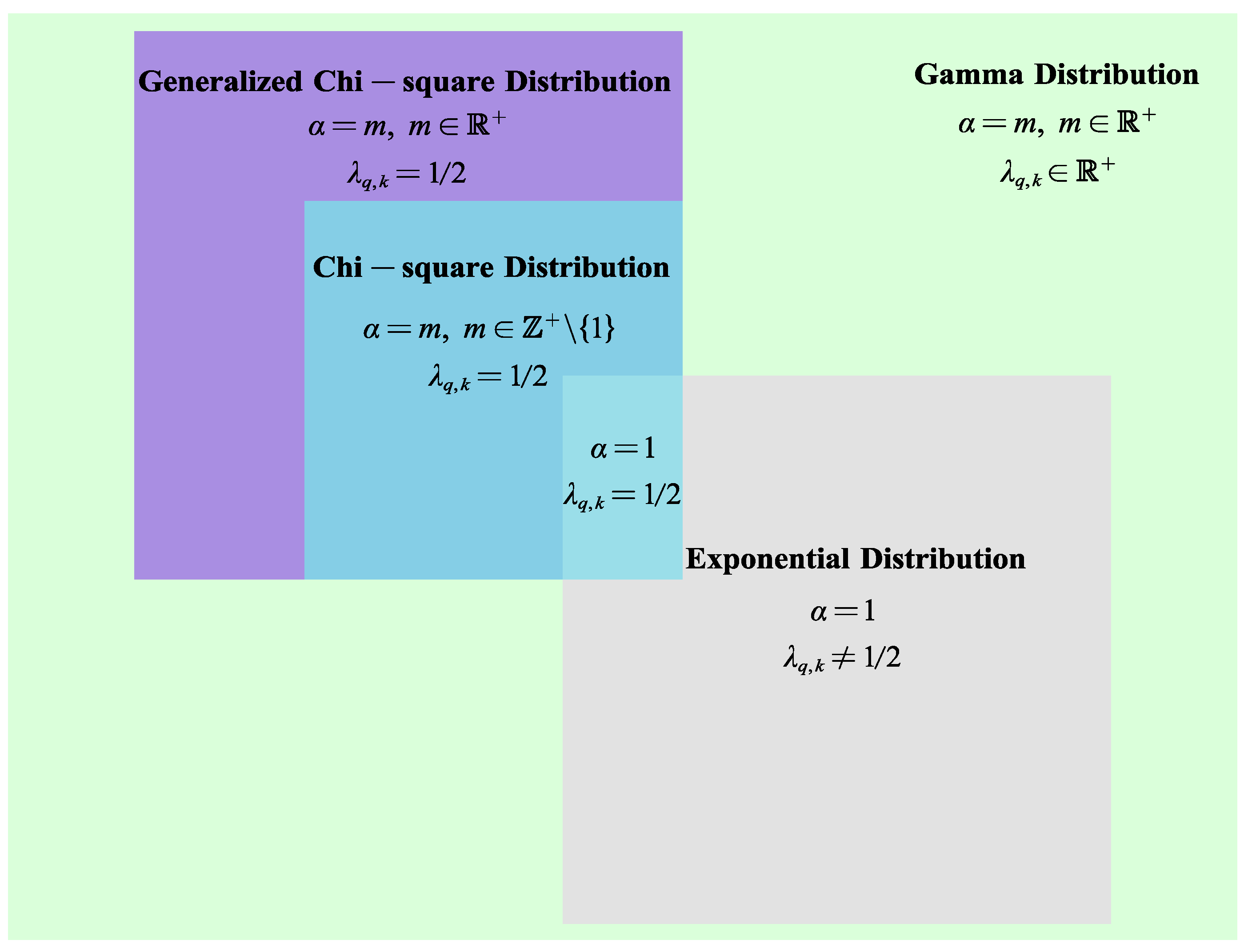
Figure 1. Relationship between Gamma distribution, Chi-square distribution, and Exponential distribution.
Remotesensing 15 01267 g001
Figure 2. Deployment of extended targets with respect to the SM-DAR.
Remotesensing 15 01267 g002
Figure 3. Variation curve of point target IRF and extended target SCIRF with m 1 , k under different P ¯ d : (a) Point Target; (b) Extended Target.
Remotesensing 15 01267 g003
Figure 4. Variation curve of point target IRF and extended target SCIRF with m 1 , k under different λ ˜ 1 , k : (a) Point Target; (b) Extended Target.
Remotesensing 15 01267 g004
Figure 5. Monotonicity of f ^ q , k ( p q , k ; 1 ) , f ^ q , k ( p q , k ; 1 ) , and f ^ q , k ( p q , k ; 1 ) in Case1: (a) Monotonicity of f ^ q , k ( p q , k ; 1 ) ; (b) Monotonicity of f ^ q , k ( p q , k ; 1 ) ; (c) Monotonicity of f ^ q , k ( p q , k ; 1 ) .
Remotesensing 15 01267 g005
Figure 6. Results for the ERCC-PA scheme and the benchmark in Case1: (a) Results of δ = 0.05 ; (b) Results of δ = 0.15 ; (c) Results of δ = 0.3 .
Remotesensing 15 01267 g006
Figure 7. Results for the ERCC-PA scheme and the benchmark in Case2, Case3, and Case4: (a) Results of α = 2 , δ = 0.05 ; (b) Results of α = 2 , δ = 0.15 ; (c) Results of α = 2 , δ = 0.3 ; (d) Results of α = 3 , δ = 0.05 ; (e) Results of α = 3 , δ = 0.15 ; (f) Results of α = 3 , δ = 0.3 ; (g) Results of α = 4 , δ = 0.05 ; (h) Results of α = 4 , δ = 0.15 ; (i) Results of α = 4 , δ = 0.3 ;.
Remotesensing 15 01267 g007
Figure 8. PDF and CDF of Gamma distribution: (a) PDF; (b) CDF.
Remotesensing 15 01267 g008
Table 1. Characteristics of function f ^ q , k ( p q , k ; α ) and constraint f ^ q , k ( p q , k ; α ) = ϑ in Case1, Case2, Case3, and Case4.
Swerling I–IISwerling III–IVWeinstock
Case1 ( α = 1 )Case2 ( α = 2 )Case3 ( α = 3 )Case4 ( α = 4 )
Degree of polynomial Equation f ^ q , k ( p q , k ; α ) = ϑ 2345
f ^ q , k ( p q , k ; α ) Transcendental Function *Y **F **FF
Existence of analytical solution of p k opt Y **F **FF
* The transcendental function here refers to a function of the form x + log(x). ** Y means to belong or exist, and F means not belong or not exist.
Table 2. Parameters of Radar.
Parameter SymbolValueMeaning
P ¯ d 0.8Probability of detection
P f a 1 × 10 6 Probability of false alarm
β q , k 2 MhzBeam width of receiver antenna
B W 1Effective bandwidth
λ ¯ q , k 2Expectation of the number n q , k of measurement values from the target
g4Gate coefficient
V q , k 400Volume of tracking gate
N M C 5 × 10 4 Monte Carlo simulation times
Table 3. Parameters of Each Target.
Target Number12345
Target Index & Symbol
Position (km) & ( x q , k , y q , k , z q , k ) (71.5, 96.4, 6)(91.1, 27, 6)(−74.6, 26, 6)(−70, 92, 6)(−1, 79, 6)
Distance (km) & D q , k 1209579115.679
Threshold of PCRLB (m) & η q 500500500500500
Expectation of RCS & ξ ¯ q , k 110.822
Table 4. Value of Extended Targets’ Global SCIRF.
Parameter NameSymbolValue
Detection Probability P ¯ d 0.30.40.50.60.70.8
Global SCIRF ϕ ¨ 1 , k , H 0.00090.00530.01550.05250.25320.9331
Table 5. Value of Point Targets’ Global IRF.
Parameter NameSymbolValue
Detection Probability P ¯ d 0.30.40.50.60.70.8
Global IRF ϕ ˙ 1 , k , L 0.02270.06480.14600.29200.52680.8986
Table 6. Total Power of ERCC-PA Scheme.
1 δ IndicatorCase1Case2Case3Case4
OASONSONSONSONS
0.95 1 T p k opt 30,410.730,410.74169.12383.71719.9
0.85 1 T p k opt 8898.48898.42248.11524.11197.8
0.70 1 T p k opt 4054.54054.51451.91102.8918.8
Table 7. Power’s Saving Rate of ERCC-PA Scheme.
1 δ Case1Case2Case3Case4
OASONSONSONSONS
0.9520.91%20.65%36.24%11.38%9.56%
0.8520.91%20.92%36.61%12.06%10.36%
0.7020.91%20.87%36.96%12.69%11.07%
Table 8. Comparison between confidence level and preset confidence level under optimal power.
1 δ Case1Case2Case3Case4
OAS 1 δ opt ONS 1 δ opt ONS 1 δ opt ONS 1 δ opt ONS 1 δ opt
0.950.95030.94980.95030.95020.9504
0.850.85040.84950.85010.85030.8503
0.700.71030.70000.70020.69960.6999
Table 9. Robustness metrics.
1 δ IndicatorCase1Case2Case3Case4
OASONSONSONSONS
0.95 ρ 0.48%0.48%0.60%0.49%0.74%
0.85 ρ 0.25%0.25%0.13%0.22%0.22%
0.70 ρ 0.01%0.01%0.07%0.14%0.04%
Disclaimer/Publisher’s Note: The statements, opinions and data contained in all publications are solely those of the individual author(s) and contributor(s) and not of MDPI and/or the editor(s). MDPI and/or the editor(s) disclaim responsibility for any injury to people or property resulting from any ideas, methods, instructions or products referred to in the content.