Novel Half-Spaces Based 3D Building Reconstruction Using Airborne LiDAR Data

Abstract

Automatic building reconstruction from laser-scanned data remains a challenging research topic due to buildings’ roof complexity and sparse data. A novel automatic building reconstruction methodology, based on half-spaces and a height jump analysis, is presented in this paper. The proposed methodology is performed in three stages. During the preprocessing stage, the classified input point cloud is clustered by position to obtain building point sets, which are then evaluated to obtain half-spaces and detect height jumps. Half-spaces represent the fundamental shape for generating building models, and their definition is obtained from the corresponding segment of points that describe an individual planar surface. The detection of height jumps is based on a DBSCAN search within a custom search space. During the second stage, the building point sets are divided into sub-buildings in such a way that their roofs do not contain height jumps. The concept of sub-buildings without height jumps is introduced to break down the complex building models with height jumps into smaller parts, where shaping with half-spaces can be applied accurately. Finally, the sub-buildings are reconstructed separately with the corresponding half-spaces and then joined back together to form a complete building model. In the experiments, the methodology’s performance was demonstrated on a large scale and validated on an ISPRS benchmark dataset, where an RMSE of 0.29 m was obtained in terms of the height difference.

1. Introduction

Automatically generated 3D building models are a vital part of various geographic information systems [1] that use the models for improving the quality of their output, such as digitalisation, analytics through simulation [2,3,4,5] and monitoring, particularly through the concept of a digital twin [6,7]. The automatic reconstruction without manual input is crucial, especially for large-scale applications, where manual 3D modelling would be impractical due to the time needed and, consequently, the related costs. Thus, a lot of research effort towards improving the building reconstruction performance has been performed in the last few years. A range of Earth Observation data can be used for the building reconstruction [8]. In this work, we focus on the reconstruction using airborne laser-scanned data, where LiDAR (Light Detection and Ranging) technology is utilised for scanning. These types of data are typically obtained by mounting a LiDAR scanner on an aircraft that flies along the area of interest.

In the conventional sense, the building reconstruction methods that use LiDAR data can be divided into three classes [9]: they can be based on data, a model or are a hybrid of the two. Considering the trend in recent years, an additional class could be included, namely a class that uses ML (Machine Learning) to generate building models [10,11].

Data-based methods can be more accurate than the rest; however, they are susceptible to errors due to noise and over- or under-segmentation. While the majority of algorithms focus on planar faces [12,13,14,15,16,17], some consider curved faces as well [18,19,20]. Li et al. [21] proposed a new methodology that links a TIN (Triangulated Irregular Network) to label maps of roof regions to create watertight polyhedral models from LiDAR data automatically. Wang et al. [22] presented a new framework on the basis of structural and closed constraints. An energy function was minimised to obtain the final 3D building surface model. Huang et al. [17] introduced a fully automatic approach for reconstructing building models with an extended hypothesis and selection-based polygonal surface reconstruction framework. They performed optimisation to ensure the correct topology and improve the recovery of details.

Model-based methods are not sensitive to noise; however, they are limited by the model library size that may not include the processed building’s roof design [23], which introduces large errors. On the other hand, a convincing roof shape is guaranteed, which makes such methods useful for visualisation purposes. Models can be generated based on a statistical analysis [24] or fitting geometric shapes while considering architectural constraints [25]. Another advantage is the applicability over low-density datasets, as demonstrated by Henn et al. [26] who applied a RANSAC-based methodology successfully on a dataset with a density of only 1.2 pts/m².

Hybrid methods try to combine both approaches to improve results. However, as they acquire the advantages, they obtain the disadvantages of the approaches as well. A popular hybrid approach is dividing buildings into smaller parts based on ridges or jump edges. Buildings’ roofs can then be fitted to parts with a lower complexity, which are then combined by 3D Boolean operations as a part of the CSG (Constructive Solid Geometry) [27,28,29,30]. Kada and Wichmann [29] generated building models with half-spaces, where the model was divided into convex parts for the subsequent unification. The concave shape was considered only for selected types of building layouts. Li et al. [30] presented a methodology for building reconstruction, which is based on combining several building primitives, which are described by parameters that were chosen as the best fit for a part of the building. The building primitives are then merged back together using a union Boolean operation. Another hybrid approach was based on variations in the Roof Topology Graph (RTG) [31,32,33] which is used for a topological description and an analysis of a building’s roof. Xiong et al. [32] demonstrated how any building roof can be described with a combination of loose edges, loose nodes and minimum cycles within an RTG, which are then used to obtain parts of a building’s roof from a predefined set of building primitives. Hu et al. [33] used a roof attribute graph for the decomposition and description of topological relations within complicated roof structures.

In our previous work [34], a parameter-free methodology was introduced for building reconstruction using half-spaces. The main limitation was the lack of support for building roofs with height jumps, which are a common occurrence, especially on a large scale. We can describe a height jump as an edge of a roof’s face, the height of which differs from a neighbouring roof’s face. This work aims to improve the original methodology to support various building roofs with planar faces. The main contributions are outlined as follows:

• A significant improvement is achieved through the division of buildings into smaller parts without height jumps, which we refer to as sub-buildings.
• The division is based on an innovative analysis of half-spaces and height jumps, where a custom search space was introduced for height jump detection. The division provides a greater ability to reconstruct building roof details, which are obtained by merging the sub-buildings.
• The height jumps and the outlines of buildings are obtained directly from the point cloud, independent of a roof’s shape, which minimises the processing errors.

This paper is organised in four sections. The next section describes the proposed methodology in detail. The results and a discussion of a large-scale application and benchmark are presented in Section 3. The final section concludes this work.

2. Methodology

The proposed methodology is performed in three stages, as shown in Figure 1. The definitions of half-spaces are obtained and height jumps are detected during data preprocessing stage (Figure 1a). The outcome of data preprocessing is used during the second stage of building division (Figure 1b). It divides buildings into sub-buildings for separate reconstruction during the final stage (Figure 1c), where they are joined to obtain the final building model. The following subsections describe the proposed stages in detail.

2.1. Data Preprocessing

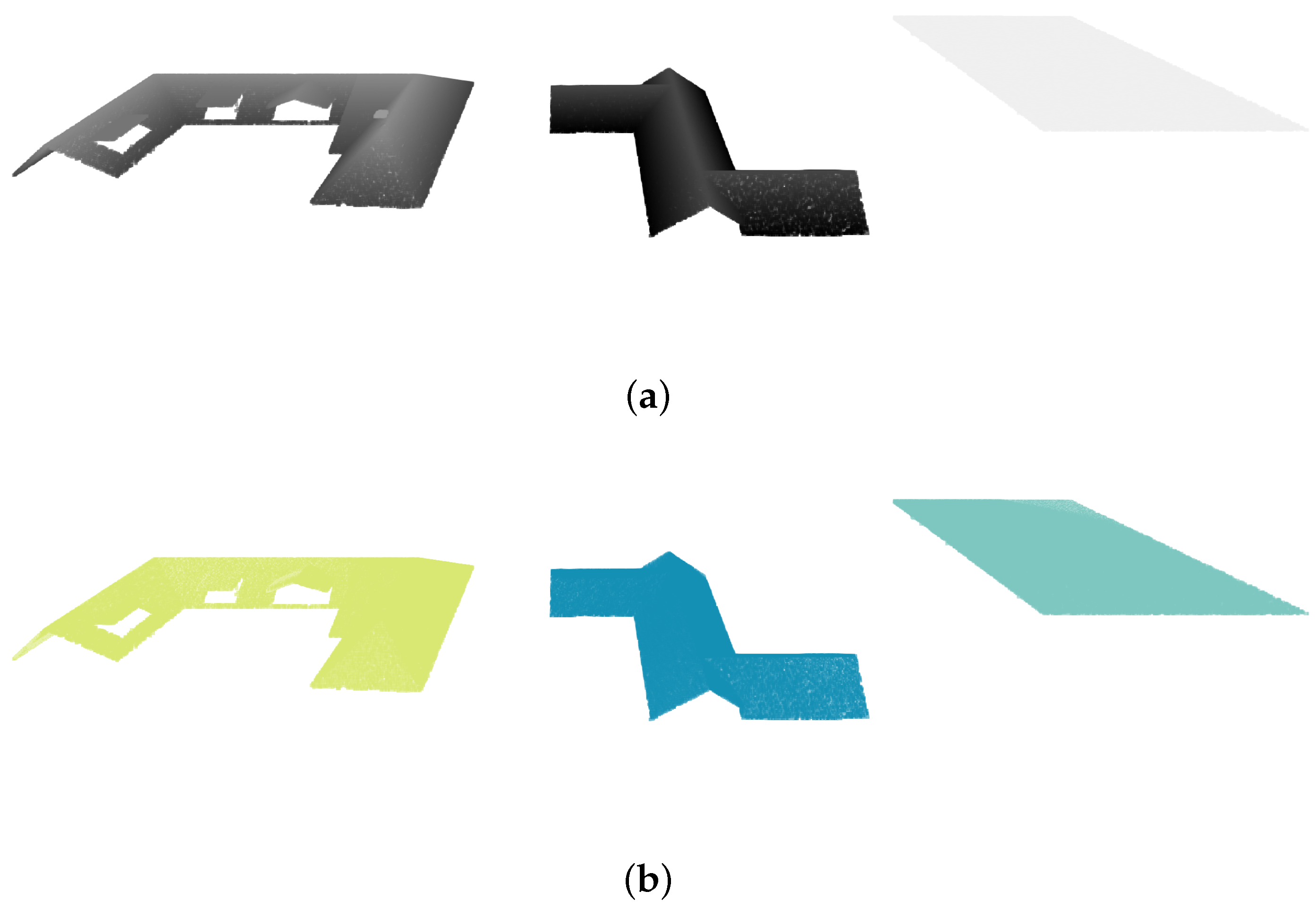
The input of the proposed reconstruction is a point cloud given as classified LiDAR data, where points are considered that are classified as a building or ground. First, the sets of building points are obtained that belong to each building. If the building outlines are available at the location, they are used for the initial division of the point cloud, where the points are arranged into smaller sets of points that are contained within each outline. For this purpose, the input LiDAR point cloud is arranged into a quad-tree structure for efficient division. This division is, however, optional and provides faster processing and helps avoid errors in the classification of the input point cloud. Independently from the availability of the building outlines, each input point cloud is processed in the same way. As distances between points from different buildings are much higher than distances between points that belong to the same building, the sets of points are determined by performing DBSCAN (Density-based Spatial Clustering of Applications with Noise) [35] by position in the Euclidean space. DBSCAN groups together those points that are closer to each other than to other groups, and its result depends on the distance $ϵ$ parameter and the minimum number of points $pt{s}_{MIN}$. The distance parameter should be set as a minimum distance, where a pair of neighbouring buildings can still be separated. In general, buildings are located several metres apart. Figure 2 shows a result of clustering by position for an example input point cloud (Figure 2a), where three separate building point sets were detected (Figure 2b). In urban settings, such building point sets usually contain several height jumps that should be located for subsequent analysis.

To detect height jumps on a point cloud directly, we designed a custom search space $HJS$ (Height Jump Space) to use within DBSCAN, where the distance between points is given as follows:

$$h_i=abs(p_i.z-p_j.z)$$

(1)

$$Dis{t}^{HJ}(p_i,p_j)=\left\{\begin{array}{cc}{h}_i& \mathrm{if}EuclDistXY(p_i,p_j)<t_{maxD}^{HJ}\mathrm{and}{h}_i>t_{height}^{HJ}\hfill \\ \infty & \mathrm{otherwise}\hfill \end{array},\right.$$

(2)

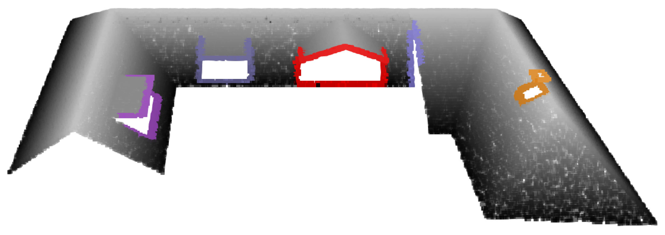
where $p_i$ and $p_j$ are points from the input point cloud, $t_{maxD}^{HJ}$ is the maximum 2D Euclidean distance threshold and $t_{height}^{HJ}$ is the minimum height difference between points that can be considered as a height jump. The proposed distance could be used independently to filter height jump candidate points; however, due to noise and inconsistent density of the point cloud, pairs of candidate points are not enough for height jump detection. Hence, DBSCAN is used to group points of the same height jump within the $HJS$ space. A set of detected height jumps that are described by the corresponding set of points for a single building point set is denoted as $J=\left\{J_i\right\}$. An example of detected height jumps within the selected building point set from Figure 2b is shown in Figure 3.

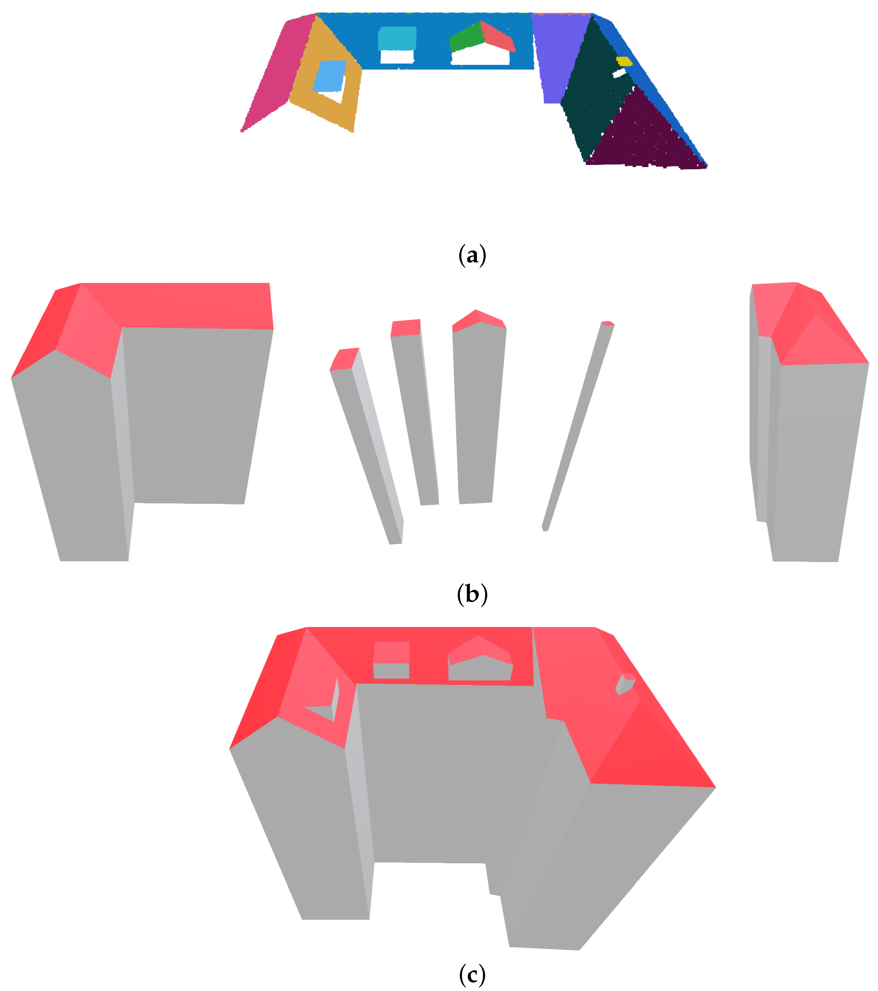
For each building point set, a set of half-spaces $H=\left\{H_j\right\}$ is obtained on the basis of a segmentation of the point cloud, where each segment is represented by a set of LiDAR points that describe individual planar roof surface [34]. Several segmentation methods are available for planar roof face extraction. Nevertheless, due to the type of input data, those that take density into account are recommended [36,37,38,39]. Each half-space $H_j$ is given as $x{f}_j.a+y{f}_j.b+z{f}_j.c+d>0$, where $f_j$ is a plane that is calculated from a set of LiDAR points $S_j$ that are contained within the corresponding segment of points. The dividing plane is obtained by least-square fitting [40] a plane to the set of LiDAR points as follows: $f_j=[a,b,c,d]=\mathrm{LSqFit}\left(S_j\right)$, where $f_j.c>0$ and LSqFit denotes the least-square fitting function. A set of obtained half-spaces for the selected building point set from Figure 2b is shown in Figure 5a. The height jumps and half-spaces are used during the second stage, referred to as building division, which is described in the next subsection.

2.2. Building Division

Buildings are divided into two stages. First, the building outlines are split using long straight height jumps, which we refer to as internal height jumps. This is followed by detecting and processing of individual half-spaces that usually represent dormers as individual buildings, during the second stage. We describe roof shapes that project out of a sloping roof as dorm-like. Figure 4 shows an example of a detected dormer height jump on the left and an internal height jump on the right.

During the division, outlines of sets of points are used at several steps and are all calculated as follows. The initial shape of an outline is calculated as an alpha shape [41], which is then processed using the established Douglas–Pecker algorithm [42] to obtain the final outline of a set of points.

The expected 2D shape of an internal height jump is a straight line segment; hence, the oriented 2D bounding box was chosen to describe the shape of such height jumps. Let $BB=\left\{B{B}_i\right\}$ be a set of 2D bounding boxes that were obtained from a set of height jumps as follows: $B{B}_i=2D\_OrientedBBox\left(J_i\right)$, where $2D\_OrientedBBox$ denotes a function that returns the 2D oriented bounding box of a set of points, where the z coordinate is neglected. In addition to the position and orientation of a 2D oriented bounding box, a $B{B}_i$ is also described by its width and length. An elongated bounding box that is of sufficient length represents a straight line shape and is, thus, suitable as an internal height jump for further processing. A different shape of a height jump would suggest a dormer-like height jump is present. On the basis of this assumption, we classify height jumps into two sets, as follows:

$$J_i\in \left\{\begin{array}{cc}{J}^I,\hfill & B{B}_i.width<2\ast t_{maxD}^{HJ}\mathrm{and}B{B}_i.length<8\ast t_{maxD}^{HJ}\hfill \\ J^D,\hfill & \mathrm{else}\hfill \end{array}\right.,$$

(3)

where $J^I\subset J$ is a set of internal height jumps and $J^D\subset J$ is a set of possible dormer-like height jumps. Width of $B{B}_i$ should be smaller than $2\ast t_{maxD}^{HJ}$ to avoid noisy or dormer-like height jumps. The internal height jump is considered long enough when it is at least four times longer than it is wide. Shorter height jumps could cause excessive splitting of a building’s outline due to an increased detection rate. For the height jumps from Figure 3, a single height jump is classified as internal (see Figure 4) and the rest are classified as dormer-like. The original outline is then split using a best-fitted (least-square fitting [40]) 2D line to the points of each $J_i\in J^I$, where the z coordinate was neglected, and it is stopped at the first segment that it hits on both sides. The result of the split is two separate building outlines that share the height jump split line. In case there are more suitable internal height jumps, the larger are processed first and the obtained smaller building outlines are split further with the internal height jumps that are contained within the corresponding outline.

Half-spaces of dormer-like roof features are then removed from the input set of half-spaces of the corresponding building and are processed separately as an independent building. A set of candidates for half-spaces with dormer-like features, denoted as $H^C\subset H$, is obtained as follows:

$$H^C=\{H_j:(f_j.c>AvgNorm\left(H\right)\left|\right|f_j.c>0.99)\mathrm{and}Area\left(\left\{H_j\right\}\right)<t_A\ast Area\left(H\right)\},$$

(4)

where $AvgNorm$ is a function that calculates the average building roof inclination normalised by area, $Area$ is a function that returns the area of the input set of half-spaces and $t_A$ limits the size of such half-spaces in regard to the entire roof to avoid cases with large, similarly inclined roof surfaces. The inclination condition was introduced based on the observation that the inclination of roof surfaces on a dormer is lower than on the rest of the roof. For cases with predominantly horizontal roofs, an additional check for horizontal half-spaces was added. For each of the candidates, we then check whether a height jump is present at its outline points and obtain the final set of half-spaces that represent dormers $H^D\subset H$:

$$H^D=\{H_j\in H^C:\exists p\in Outline\left(S_j\right)\mathrm{and}p\in J_k,J_k\in J^D\},$$

(5)

where $Outline$ is a function that yields the outline of a set of points. As dormers can be shaped by multiple half-spaces, such as the case for the dormer height jump in Figure 4, dormer half-spaces $H_j\in H^D$ that share a height jump with another $H_l\in H^D,j\ne l$ are grouped together with a common outline.

The remaining set of half-spaces $H\setminus H^D$ are associated with the corresponding outline using the point-in-polygon test. A set of outlines and the corresponding half-spaces represent the input for generating sub-building models in the next step.

2.3. Shaping 3D Building Models

In this step, a single watertight 3D building model is generated from a set of sub-buildings, which are denoted as $B=\left\{B_m\right\}$. Each sub-building is generated from an outline and its corresponding half-spaces using the methodology from our previous work that was based on 3D Boolean operations [34] and is performed as follows. First, a base model $B_m$ is generated with vertical walls and a flat horizontal roof, where the building outline is set at the height of the lowest nearby ground LiDAR point as the floor, and the top horizontal roof of the same building outline shape is put above the highest building LiDAR point. The model $B_m$ is then shaped with a combination of half-spaces and 3D Boolean operations, where the half-spaces are classified as follows [34]:

$$H_j\in \left\{\begin{array}{cc}{H}^O,\hfill & \exists p\in S_k:p\in H_j,k\ne j\hfill \\ H^U,\hfill & \mathrm{else}\hfill \end{array}\right.,$$

(6)

where $H^O\subset H$ is a set of obstructed half-spaces, and $H^U\subset H$ is a set of unobstructed half-spaces. Unobstructed half-spaces contain no points from other half-spaces and describe the convex part of the building model. Therefore, they can be used directly to shape the model by subtracting them from the base model [34]:

$$\forall H_n\in H^U:B_m=B_m\setminus H_n$$

(7)

Obstructed half-spaces contain points from other half-spaces and, thus, are processed further to generate slices for concave parts of the roof that are cut from the base model [34]:

$$\forall H_o\in H^O:B_m=B_m\backslash s_o,$$

(8)

where $s_o$ is a slice that is obtained by intersecting $H_o$ with all other $H_p\in H^O$, $o\ne p$, that are visible from $H_o$. For more details, see [34]. Once all sub-buildings are generated, they are merged using a union 3D Boolean operation to obtain the final building model:

$$\forall B_m\in B:W=W\cup B_m,$$

(9)

where W is the final watertight building model that was initialised as an empty set. Figure 5c shows an example of a generated final building model with sub-buildings that are shown in Figure 5b.

3. Results and Discussion

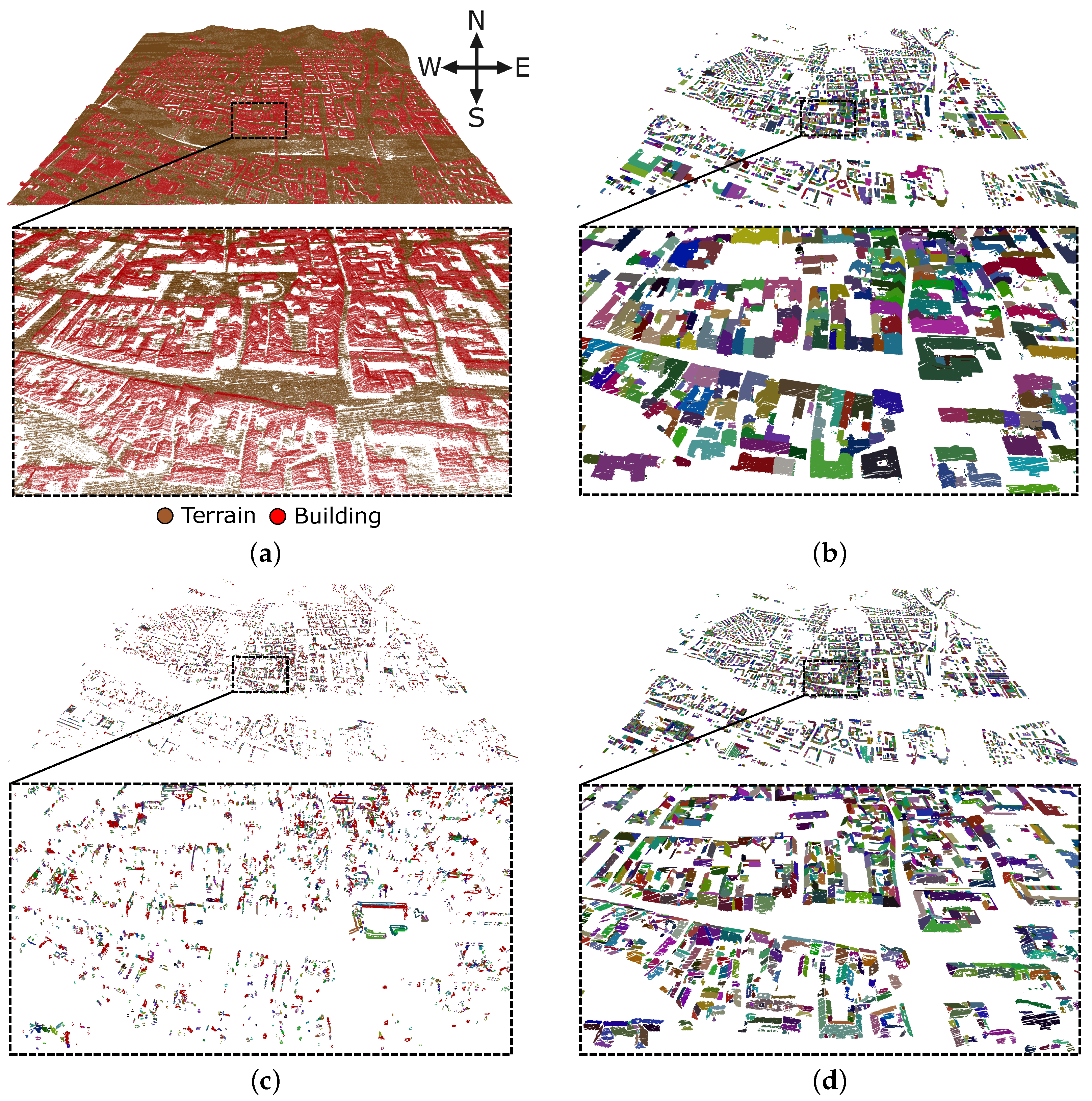
The large-scale applicability of the algorithm was tested on a LiDAR dataset that covers a 6.153 km² geographic area of the city of Maribor, Slovenia (altitude: 275 m, bounding box: 46°33^′8.5430^″N 15°37^′29.2311^″E, 46°34^′13.1557^″N 15°39^′52.9794^″E). Figure 6a shows the dataset, which contains 14,227,123 buildings and 31,420,386 ground points, with an average density of 11.3 pts/m². The dataset was obtained in 2014 using a LiDAR scanner mounted on an aeroplane. The area of the dataset was selected as it contains diverse building types, such as buildings from an old city centre, modern high-rise buildings, as well as single-family houses in the suburbs.

First, the building point set was estimated for each building. Even though building outlines are not required as an input, they were used for the demonstrated large-scale reconstruction in this section, as in the city centre multiple buildings can share geometrically highly similar roof faces. In addition, outlines help avoid errors in the classified input point cloud, for example, bridges classified as buildings. Therefore, the building points were first divided with an existing dataset of building outlines that were obtained from a public database by The Surveying and Mapping Authority of the Republic of Slovenia. Using outlines for generating the model directly was not considered, as usually there are several sub-buildings with their own outlines contained within each building point set that only partially align with the outlines from the public dataset. However, the use of publicly available outlines would definitely be beneficial if the further simplification of building outlines was required. For estimating building point sets, the maximum distance between points $ϵ$ was set to 2 m, and at least 5 points were required to form a building point set. A lower $ϵ$ might result in the grouping of points from neighbouring buildings due to noise, which could cause reconstruction errors due to an unexpected roof shape. The result of such a segmentation is shown in Figure 6b, where the building point sets’ colours were chosen randomly. These point sets were then processed to detect height jumps and obtain the definition of half-spaces. For the height jump detection, the settings used are given in

Table 1. Parameters used for the detection of height jumps.

Parameter	Value
$t_{maxD}^{HJ}$	0.9
$t_{height}^{HJ}$	2.0
$pt{s}_{MIN}$	5

.

The parameters used for this step are set empirically and are highly dependent on the characteristics of the input point cloud, namely the density and accuracy. For example, the maximum 2D distance $t_{maxD}^{HJ}$ depends on the distance between neighbouring scan lines, and it should be set to contain at least two neighbouring scan lines in the LiDAR data. In case $t_{maxD}^{HJ}$ would not contain two scan lines, height jumps would not be detected correctly. Others are set in line with the desired complexity of the building models. A too low $t_{height}^{HJ}$ could result in the detection of points at an entire roof face as a height jump, which is why it should be set higher than $t_{maxD}^{HJ}$. Figure 6c shows the results of the height jump detection over the segments of the points from Figure 6b. The definition of half-spaces was obtained on the basis of a graph-based segmentation [37] that takes the point cloud density and local curvature of faces into account. It should be noted that a different method can be chosen for the segmentation of planar faces, as suggested in the original methodology [34]. The selected segmentation was performed using the settings given in

Table 2. Parameters used for segmentation of the point cloud.

Parameter	Value
k	20
$t_{\theta }$	2.5
$t_{CC}$	50
$t_d$ (m)	2

. At least 50 points were required for each segment ($t_{CC}=50$), which was set to avoid faces smaller than approximately 4.5 m². The estimated segmentation over the building point sets from Figure 6b is shown in Figure 6d.

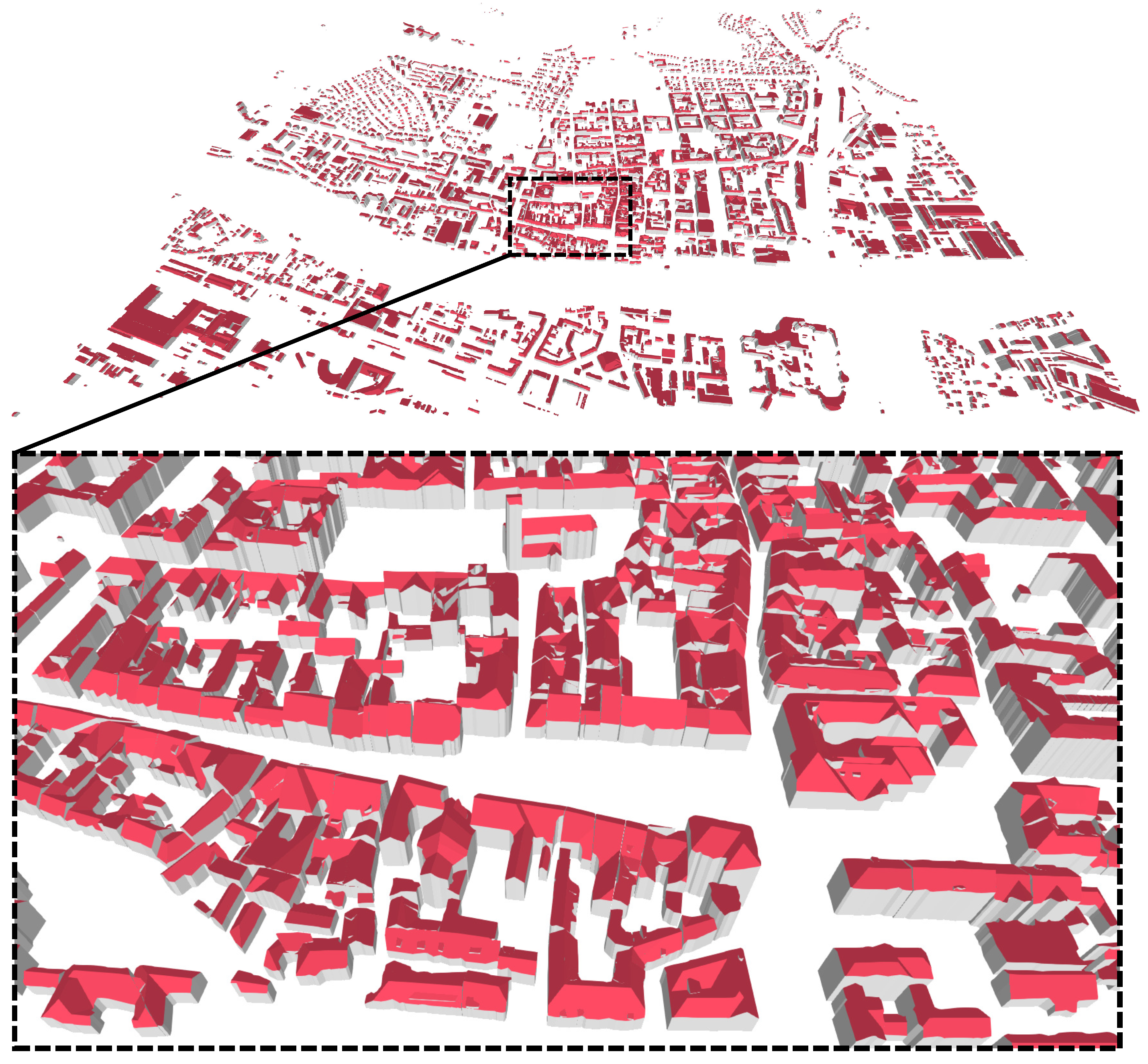
After the next step, the preprocessed data of each building point set was divided into smaller sets as sub-buildings for a separate reconstruction, where a $t_A$ value of 0.3 provided the best results. A low $t_A$ might result in some dormers being neglected. Higher values, however, would allow large, similarly inclined roof surfaces to be processed as dormers, which could cause an incorrect reconstruction. The obtained sub-buildings were then joined together for the final building models. The resulting reconstruction that includes 5383 building models is shown in Figure 7.

We examine typical building cases included in the city model from Figure 7 in more detail, as shown in Figure 8. For each case, an orthophoto of the building is shown on the top, followed by the input point cloud and intermediary results by the performed steps of the proposed methodology. Finally, the reconstructed building model is provided at the bottom. The first case (Figure 8a) is a church with a multi-level roof that includes a bell tower. With the first step of the clustering by position, the methodology was able to split the building into sub-buildings without height jumps, which were then merged after the separate reconstruction. The next case represents an example of high-rise buildings, as shown in Figure 8b. For this case, the clustering by position was not able to split all the buildings into sets of points without height jumps due to the noise and errors in the classification, as building points were present on the walls between the horizontal roof surfaces at different heights. A correct reconstruction was ensured by building division, where the top half-spaces were processed as sub-buildings, and by building outline division, where an internal height jump was used to split the outline of the leftmost building point set. The final case (Figure 8c) is a more complex building model with multiple height jumps, as it includes several towers and dormers. The largest height jumps were solved with the clustering by position, whereas during the building division, the sub-buildings without height jumps were obtained with the separation of half-spaces that represent dormer-like features from the initial half-spaces set.

3.1. Validation

The validation was performed with a manually classified and established benchmark dataset provided by the International Society for Photogrammetry and Remote Sensing (ISPRS), specifically the third area of the data obtained over Vaihingen, Germany [43,44]. The performance of the proposed algorithm can be inspected in Figure 9, where the height difference to the ground-truth data from the benchmark is shown. A regular grid with a 0.1 m resolution was used for the height difference estimation. The results are given in

Table 3. Validation of the obtained results from the comparison with the ISPRS benchmark data.

Metric	Value
RMSE (m)	0.29
Completeness (%)	85.0
$e_{0.5}$ (%)	96.9

. The RMSE (Root Mean Square Error) was estimated over the height differences, the proportion of the building area covered by the generated building models is given by completeness and the proportion of the building area, where the height difference is lower than 0.5 m, is designated by $e_{0.5}$.

It can be observed (see Figure 9) that, in the majority of the compared area, the height difference is minimal, which demonstrates the accuracy of the reconstruction. The height differences can be observed in small objects (e.g., chimneys), parts of the dataset with a lower density, and locations where segmented planar faces were either merged together or smaller than the original.

Some chimneys were reconstructed accurately, which can be observed on the top right building. The main issue with chimneys and other small objects was an insufficient number of points at the surface to detect a planar roof face reliably. The reconstruction of a building with a significantly lower point cloud density than the rest of the buildings, for example, the case of a building located near the top of the input benchmark dataset, can produce incorrect results already at the first step of the clustering by position. The difficulties with the selected segmentation for planar roof face detection can be attributed to the noise and insufficient local curvature at neighbouring roof faces.

In comparison with the original methodology [34] that did not consider height jumps, the height difference in terms of the RMSE has been lowered significantly by more than 1 m. On the other hand, the completeness is lower for the improved methodology, which can be attributed to the absence of building outlines as an input to the improved methodology. On parts of the input point cloud with a low density, no building models were generated in contrast with the original methodology that already expected building faces within the outline. On the other hand, the proportion of the building area, where the height difference is lower than 0.5 m, was improved significantly by a nominal 17.5%, which further verifies the improved accuracy of the proposed methodology. When comparing the results with the other related work, the proposed methodology matched the best result reported by the ISPRS benchmark results [44] and the work by Hu et al. [33] in terms of the height difference provided by the RMSE. Together with a sufficient completeness, the methodology’s performance is considered validated.

3.2. Limitations

The methodology is highly dependent on the quality of the input LiDAR data, which may not be available at a desired location. Geometrically, the quality of a point cloud is characterised by the density and accuracy of the point cloud, both of which affect the quality of the output building model significantly [45]. Semantically, the quality is associated with errors in the classification of the building point cloud, which are a common occurrence, especially on a large scale.

Even though it is highly effective for most building roofs, the filtration of half-spaces for dormer-like features, which is based on the average inclination normalised by area, may miss some half-spaces due to their size or skewed average inclination values. Furthermore, it is acknowledged that the outline processing could be improved further through rectangularisation and parallelisation. However, it is a separate challenge that could introduce additional errors in the building shape. In cases of splitting the building outline with an internal height jump, it is possible that the split of the building outline extends well over the bounds of the internal jump size. However, due to the union of sub-buildings at the end of the methodology, such a split, or multiple splits, generally does not represent an issue. It could pose a problem if the split line would traverse so close to a building outline that a half-space would not be included in the narrow part of the outline.

4. Conclusions

This paper presented a novel methodology for automatic building reconstruction from LiDAR data based on half-spaces, where height jumps were considered. It is a significant upgrade over our previous work and is performed in three stages, where during the first stage the input LiDAR point cloud is preprocessed to obtain sets of points of individual buildings, which are then processed further for the detection of height jumps and half-spaces. In the second stage, the buildings are divided into sub-buildings with roofs without height jumps, which are then joined back together after a separate building reconstruction during the final stage.

In the experiments, the proposed methodology was applied on a large scale, where most of the urban area was reconstructed sufficiently. A comparison with the related work revealed a high accuracy that matched the best result in terms of the height difference from the ISPRS benchmark. The methodology’s performance is limited by the quality of the input point cloud, and it was acknowledged that the building division may not yield sub-buildings without any height jumps in all cases. The filtration of the candidates for dormer-like features could be explored further, particularly through Machine Learning.

It was demonstrated that it is possible to achieve a highly accurate building reconstruction using half-spaces and the corresponding height jump analysis. The large-scale applicability of the presented methodology makes it beneficial for any type of 3D urban analysis, simulation or monitoring solution.

References

1. Liu, P.; Biljecki, F. A review of spatially-explicit GeoAI applications in Urban Geography. Int. J. Appl. Earth Obs. Geoinf. 2022, 112, 102936. [Google Scholar] [CrossRef]
2. Hofierka, J.; Gallay, M.; Onačillová, K.; Hofierka, J. Physically-based land surface temperature modeling in urban areas using a 3-D city model and multispectral satellite data. Urban Clim. 2020, 31, 100566. [Google Scholar] [CrossRef]
3. Bizjak, M.; Žalik, B.; Štumberger, G.; Lukač, N. Large-scale estimation of buildings’ thermal load using LiDAR data. Energy Build. 2021, 231, 110626. [Google Scholar] [CrossRef]
4. Ali, U.; Shamsi, M.H.; Hoare, C.; Mangina, E.; O’Donnell, J. Review of urban building energy modeling (UBEM) approaches, methods and tools using qualitative and quantitative analysis. Energy Build. 2021, 246, 111073. [Google Scholar] [CrossRef]
5. Yuan, J.; Masuko, S.; Shimazaki, Y.; Yamanaka, T.; Kobayashi, T. Evaluation of outdoor thermal comfort under different building external-wall-surface with different reflective directional properties using CFD analysis and model experiment. Build. Environ. 2022, 207, 108478. [Google Scholar] [CrossRef]
6. Deng, T.; Zhang, K.; Shen, Z.J.M. A systematic review of a digital twin city: A new pattern of urban governance toward smart cities. J. Manag. Sci. Eng. 2021, 6, 125–134. [Google Scholar] [CrossRef]
7. Pang, H.E.; Biljecki, F. 3D building reconstruction from single street view images using deep learning. Int. J. Appl. Earth Obs. Geoinf. 2022, 112, 102859. [Google Scholar] [CrossRef]
8. Wang, R. 3D building modeling using images and LiDAR: A review. Int. J. Image Data Fusion 2013, 4, 273–292. [Google Scholar] [CrossRef]
9. Wang, R.; Peethambaran, J.; Dong, C. LiDAR Point Clouds to 3D Urban Models: A Review. IEEE J. Sel. Top. Appl. Earth Obs. Remote. Sens. 2018, 11, 606–627. [Google Scholar] [CrossRef]
10. Buyukdemircioglu, M.; Kocaman, S.; Kada, M. Deep learning for 3D building reconstruction: A review. Int. Arch. Photogramm. Remote Sens. Spat. Inf. Sci. 2022, XLIII-B2-2, 359–366. [Google Scholar] [CrossRef]
11. Li, L.; Song, N.; Sun, F.; Liu, X.; Wang, R.; Yao, J.; Cao, S. Point2Roof: End-to-end 3D building roof modeling from airborne LiDAR point clouds. ISPRS J. Photogramm. Remote Sens. 2022, 193, 17–28. [Google Scholar] [CrossRef]
12. Dorninger, P.; Pfeifer, N. A Comprehensive Automated 3D Approach for Building Extraction, Reconstruction, and Regularization from Airborne Laser Scanning Point Clouds. Sensors 2008, 8, 7323–7343. [Google Scholar] [CrossRef] [Green Version]
13. Elberink, S.O.; Vosselman, G. Building reconstruction by target based graph matching on incomplete laser data: Analysis and limitations. Sensors 2009, 9, 6101–6118. [Google Scholar] [CrossRef] [PubMed] [Green Version]
14. Sampath, A.; Shan, J. Segmentation and reconstruction of polyhedral building roofs from aerial LiDAR point clouds. IEEE Trans. Geosci. Remote Sens. 2010, 48, 1554–1567. [Google Scholar] [CrossRef]
15. Chen, Y.; Cheng, L.; Li, M.; Wang, J.; Tong, L.; Yang, K. Multiscale grid method for detection and reconstruction of building roofs from airborne LiDAR data. IEEE J. Sel. Top. Appl. Earth Obs. Remote Sens. 2014, 7, 4081–4094. [Google Scholar] [CrossRef]
16. Chen, D.; Wang, R.; Peethambaran, J. Topologically Aware Building Rooftop Reconstruction From Airborne Laser Scanning Point Clouds. IEEE Trans. Geosci. Remote Sens. 2017, 55, 7032–7052. [Google Scholar] [CrossRef]
17. Huang, J.; Stoter, J.; Peters, R.; Nan, L. City3D: Large-Scale Building Reconstruction from Airborne LiDAR Point Clouds. Remote Sens. 2022, 14, 2254. [Google Scholar] [CrossRef]
18. Lafarge, F.; Mallet, C. Creating large-scale city models from 3D-point clouds: A robust approach with hybrid representation. Int. J. Comput. Vis. 2012, 99, 69–85. [Google Scholar] [CrossRef] [Green Version]
19. Zhou, Q.Y.; Neumann, U. 2.5D building modeling by discovering global regularities. In Proceedings of the IEEE Computer Society Conference on Computer Vision and Pattern Recognition, Providence, RI, USA, 16–21 June 2012; pp. 326–333. [Google Scholar] [CrossRef]
20. Bauchet, J.P.; Lafarge, F. Kinetic Shape Reconstruction. ACM Trans. Graph. 2020, 39, 1–4. [Google Scholar] [CrossRef]
21. Li, M.; Rottensteiner, F.; Heipke, C. Modelling of buildings from aerial LiDAR point clouds using TINs and label maps. ISPRS J. Photogramm. Remote Sens. 2019, 154, 127–138. [Google Scholar] [CrossRef]
22. Wang, S.; Cai, G.; Cheng, M.; Marcato Junior, J.; Huang, S.; Wang, Z.; Su, S.; Li, J. Robust 3D reconstruction of building surfaces from point clouds based on structural and closed constraints. ISPRS J. Photogramm. Remote Sens. 2020, 170, 29–44. [Google Scholar] [CrossRef]
23. Vosselman, G. Building Reconstruction Using Planar Faces In Very High Density Height Data. Int. Arch. Photogramm. Remote Sens. 1999, 32, 87–92. [Google Scholar]
24. Huang, H.; Brenner, C.; Sester, M. A generative statistical approach to automatic 3D building roof reconstruction from laser scanning data. ISPRS J. Photogramm. Remote Sens. 2013, 79, 29–43. [Google Scholar] [CrossRef]
25. Poullis, C.; You, S. Photorealistic large-scale Urban city model reconstruction. IEEE Trans. Vis. Comput. Graph. 2009, 15, 654–669. [Google Scholar] [CrossRef]
26. Henn, A.; Gröger, G.; Stroh, V.; Plümer, L. Model driven reconstruction of roofs from sparse LIDAR point clouds. ISPRS J. Photogramm. Remote Sens. 2013, 76, 17–29. [Google Scholar] [CrossRef]
27. Haala, N.; Brenner, C. Virtual city models from laser altimeter and 2D map data. Photogramm. Eng. Remote Sens. 1999, 65, 787–795. [Google Scholar]
28. Kada, M.; McKinley, L. 3D Building Reconstruction from LIDAR based on a Cell Decomposition Approach. In Proceedings of the CMRT09: Object Extraction for 3D City Models, Road Databases and Traffic Monitoring-Concepts, Algorithms and Evaluation, Paris, France, 3–4 September 2009; Volume XXXVIII, pp. 47–52. [Google Scholar]
29. Kada, M.; Wichmann, A. Feature-Driven 3d Building Modeling Using Planar Halfspaces. ISPRS Ann. Photogramm. Remote Sens. Spat. Inf. Sci. 2013, II-3/W3, 37–42. [Google Scholar] [CrossRef] [Green Version]
30. Li, Z.; Shan, J. RANSAC-based multi primitive building reconstruction from 3D point clouds. ISPRS J. Photogramm. Remote Sens. 2022, 185, 247–260. [Google Scholar] [CrossRef]
31. Verma, V.; Kumar, R.; Hsu, S. 3D Building Detection and Modeling from Aerial LiDAR Data. In Proceedings of the 2006 IEEE Computer Society Conference on Computer Vision and Pattern Recognition, New York, NY, USA, 17–22 June 2006; Volume 2, pp. 2213–2220. [Google Scholar] [CrossRef]
32. Xiong, B.; Jancosek, M.; Oude Elberink, S.; Vosselman, G. Flexible building primitives for 3D building modeling. ISPRS J. Photogramm. Remote Sens. 2015, 101, 275–290. [Google Scholar] [CrossRef]
33. Hu, P.; Yang, B.; Dong, Z.; Yuan, P.; Huang, R.; Fan, H.; Sun, X. Towards Reconstructing 3D Buildings from ALS Data Based on Gestalt Laws. Remote Sens. 2018, 10, 1127. [Google Scholar] [CrossRef] [Green Version]
34. Bizjak, M.; Žalik, B.; Lukač, N. Parameter-Free Half-Spaces Based 3D Building Reconstruction Using Ground and Segmented Building Points from Airborne LiDAR Data with 2D Outlines. Remote Sens. 2021, 13, 4430. [Google Scholar] [CrossRef]
35. Ester, M.; Kriegel, H.; Sander, J.; Xu, X. A density-based algorithm for discovering clusters in large spatial databases with noise. In Proceedings of the Second International Conference on Knowledge Discovery and Data Mining (KDD-96), Portland, OR, USA, 2–4 August 1996; AAAI Press: Palo Alto, CA, USA, 1996; Volume 96, pp. 226–231. [Google Scholar]
36. Rabbani, T.; den Heuvel, F.; Vosselmann, G. Segmentation of point clouds using smoothness constraint. Int. Arch. Photogramm. Remote Sens. Spat. Inf. Sci. 2006, 36, 248–253. [Google Scholar]
37. Bizjak, M. The segmentation of a point cloud using locally fitted surfaces. In Proceedings of the 18th Mediterranean Electrotechnical Conference: Intelligent and Efficient Technologis and Services for the Citizen, MELECON 2016, Lemesos, Cyprus, 18–20 April 2016; IEEE: Limassol, Cyprus, 2016; pp. 1–6. [Google Scholar] [CrossRef]
38. Czerniawski, T.; Sankaran, B.; Nahangi, M.; Haas, C.; Leite, F. 6D DBSCAN-based segmentation of building point clouds for planar object classification. Autom. Constr. 2018, 88, 44–58. [Google Scholar] [CrossRef]
39. Li, L.; Yao, J.; Tu, J.; Liu, X.; Li, Y.; Guo, L. Roof plane segmentation from airborne LiDAR data using hierarchical clustering and boundary relabeling. Remote Sens. 2020, 12, 1363. [Google Scholar] [CrossRef]
40. Bevington, P.R.; Robinson, D.K. Data Reduction and Error Analysis for the Physical Sciences, 3rd ed.; McGraw–Hill: New York, NY, USA, 2002. [Google Scholar]
41. Edelsbrunner, H.; Kirkpatrick, D.; Seidel, R. On the shape of a set of points in the plane. IEEE Trans. Inf. Theory 1983, 29, 551–559. [Google Scholar] [CrossRef] [Green Version]
42. Douglas, D.H.; Peucker, T.K. Algorithms for the reduction of the number of points required to represent a digitized line or its caricature. Cartogr. Int. J. Geogr. Inf. Geovisualization 1973, 10, 112–122. [Google Scholar] [CrossRef] [Green Version]
43. Cramer, M. The DGPF-Test on Digital Airborne Camera Evaluation Overview and Test Design. Photogramm.-Fernerkund.-Geoinf. 2010, 2010, 73–82. [Google Scholar] [CrossRef]
44. Rottensteiner, F.; Sohn, G.; Jung, J.; Gerke, M.; Baillard, C.; Benitez, S.; Breitkopf, U. The ISPRS benchmark on urban object classification and 3D building reconstruction. ISPRS Ann. Photogramm. Remote Sens. Spat. Inf. Sci. 2012, I-3, 293–298. [Google Scholar] [CrossRef] [Green Version]
45. Biljecki, F.; Heuvelink, G.B.; Ledoux, H.; Stoter, J. The effect of acquisition error and level of detail on the accuracy of spatial analyses. Cartogr. Geogr. Inf. Sci. 2018, 45, 156–176. [Google Scholar] [CrossRef] [Green Version]
Figure 1. Workflow of the proposed methodology: data preprocessing (a), building division (b) and shaping 3D building models (c).
Remotesensing 15 01269 g001
Figure 2. Illustration of clustering a point cloud by position, where the input points on top (a) are coloured by their height and the points in the bottom (b) in regard to which building point set they correspond to.
Remotesensing 15 01269 g002
Figure 3. Detected height jumps for the first building point set on the left in Figure 2b, where points of each height jump are coloured.
Remotesensing 15 01269 g003
Figure 4. Visualisation of both types of considered height jumps, where the corresponding points of a dormer height jump are red, and the points of an internal height jump from Figure 3 are violet.
Remotesensing 15 01269 g004
Figure 5. Illustration of generating building model, where the input half-spaces are shown on the top (a), the obtained sub-buildings are shown in the middle (b), and (c) shows the final building model that was obtained by a union of all sub-buildings.
Remotesensing 15 01269 g005
Figure 6. Illustration of input data processing, where (a) shows the input LiDAR point cloud acquired over Maribor (Slovenia), (b) building point sets obtained with clustering by position, (c) detected height jumps and (d) segmented planar faces over segments from (b).
Remotesensing 15 01269 g006
Figure 7. Reconstructed city model for the height jumps and segmented planar faces from Figure 6c and Figure 6d, respectively.
Remotesensing 15 01269 g007
Figure 8. Illustrations of the reconstruction of buildings of various types, where for the buildings' (top) input point cloud and subsequent intermediate results of the proposed methodology's steps are shown for the reconstructed building models (bottom). (a) is a church with a multi-level roof, (b) is an example of high-rise buildings, and (c) is a complex building model with multiple height jumps.
Remotesensing 15 01269 g008
Figure 9. Height difference comparison of the output of the proposed algorithm with the ground-truth data of the ISPRS benchmark.
Remotesensing 15 01269 g009