

Sensor-Aided Calibration of Relative Extrinsic Parameters for Outdoor Stereo Vision Systems


Abstract
1. Introduction
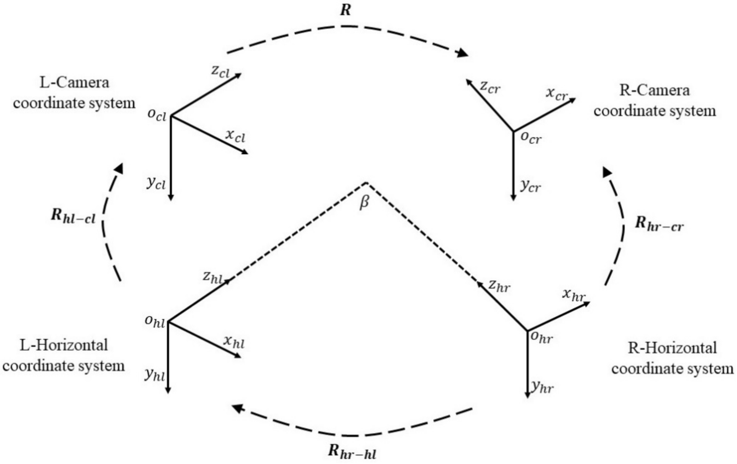
2. Methodology
3. Experiments and Results
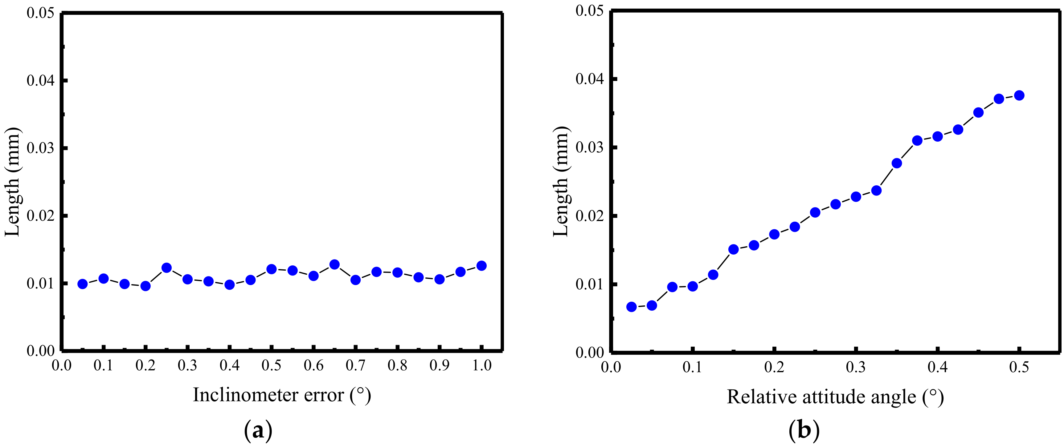
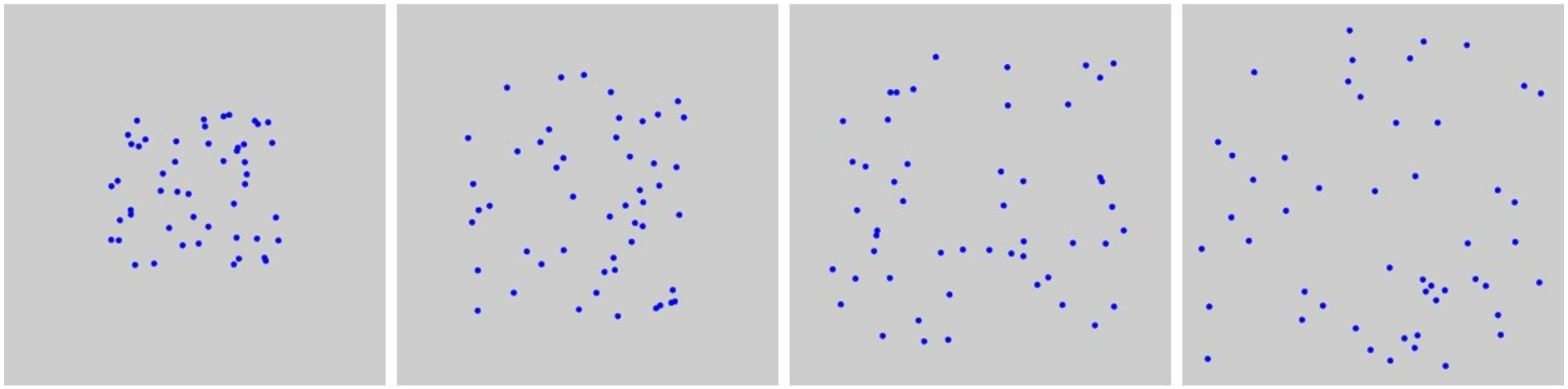
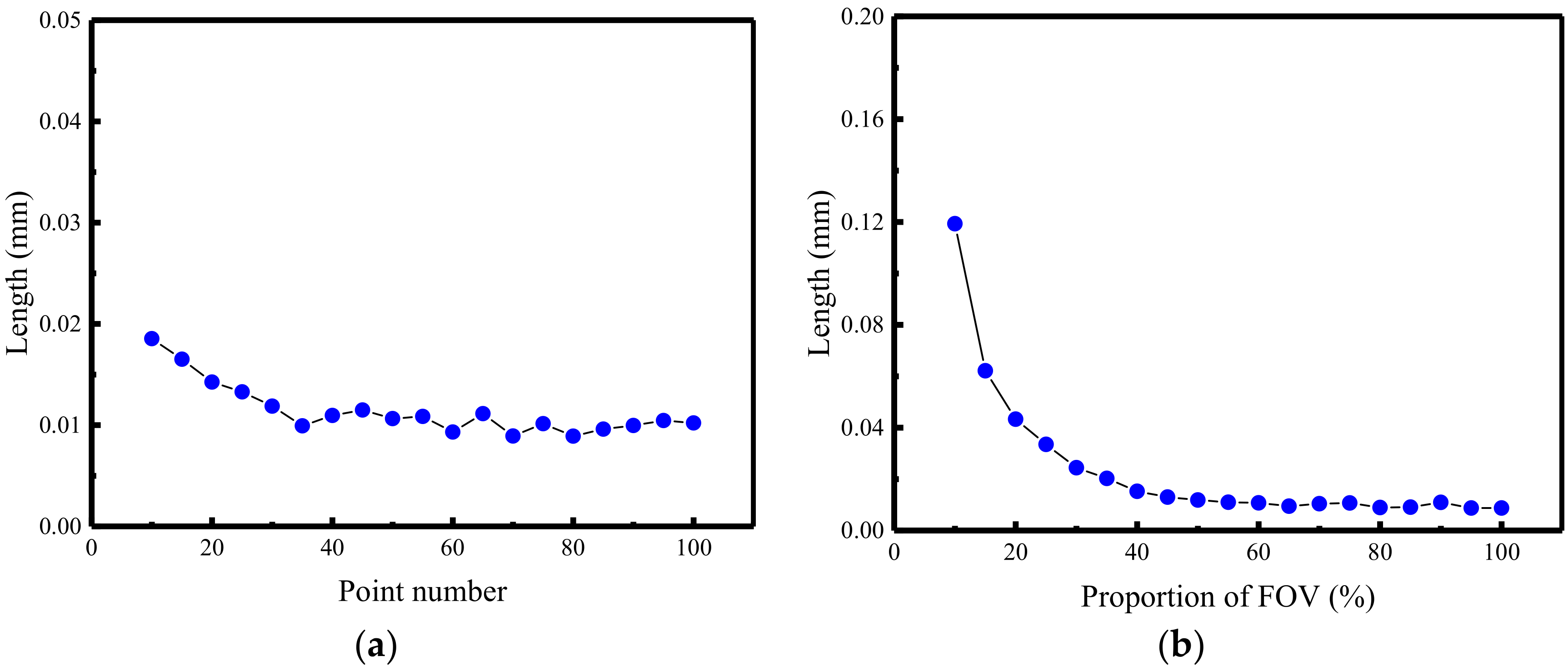
3.1. Simulation
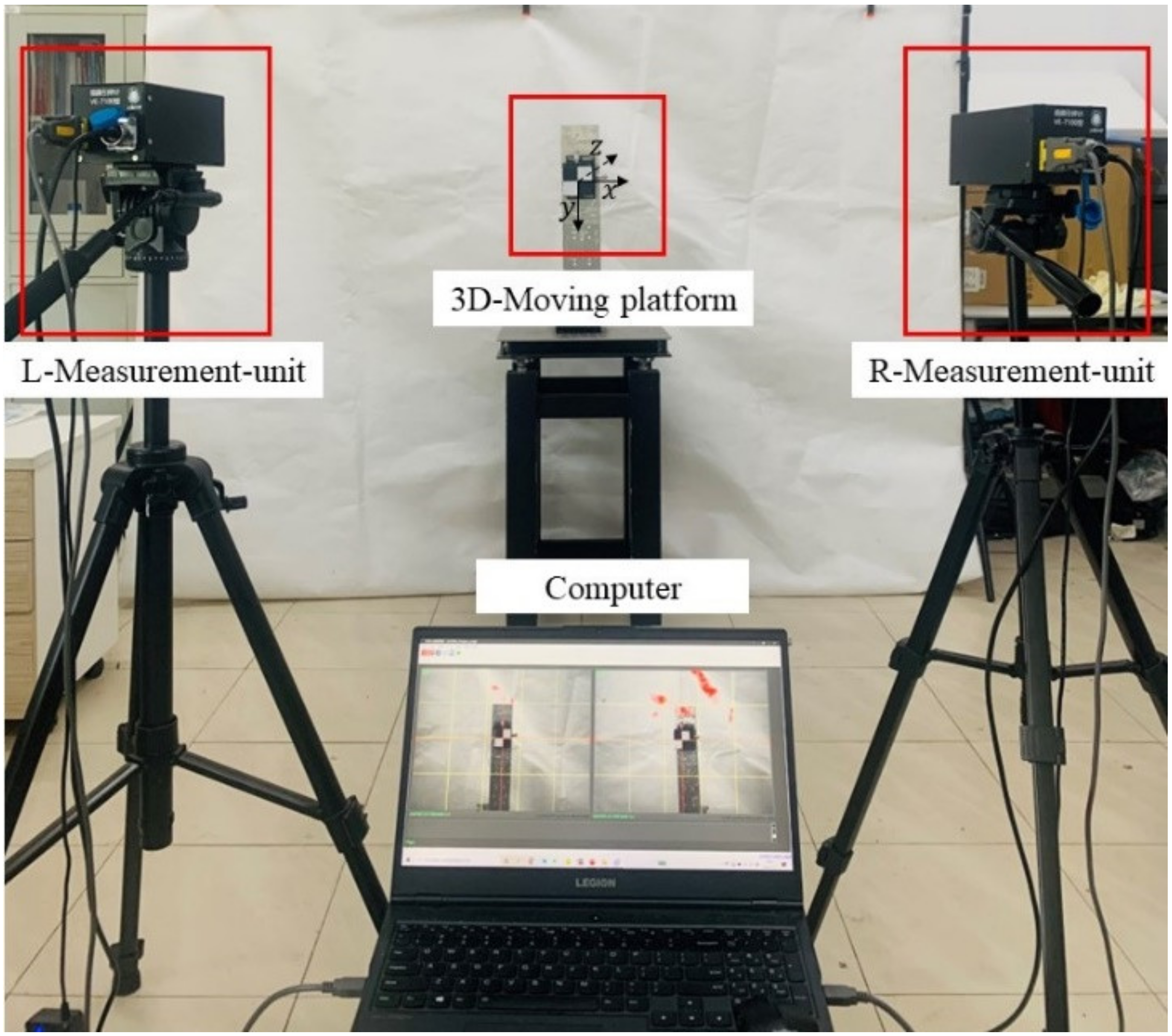
3.2. Experimental Validation
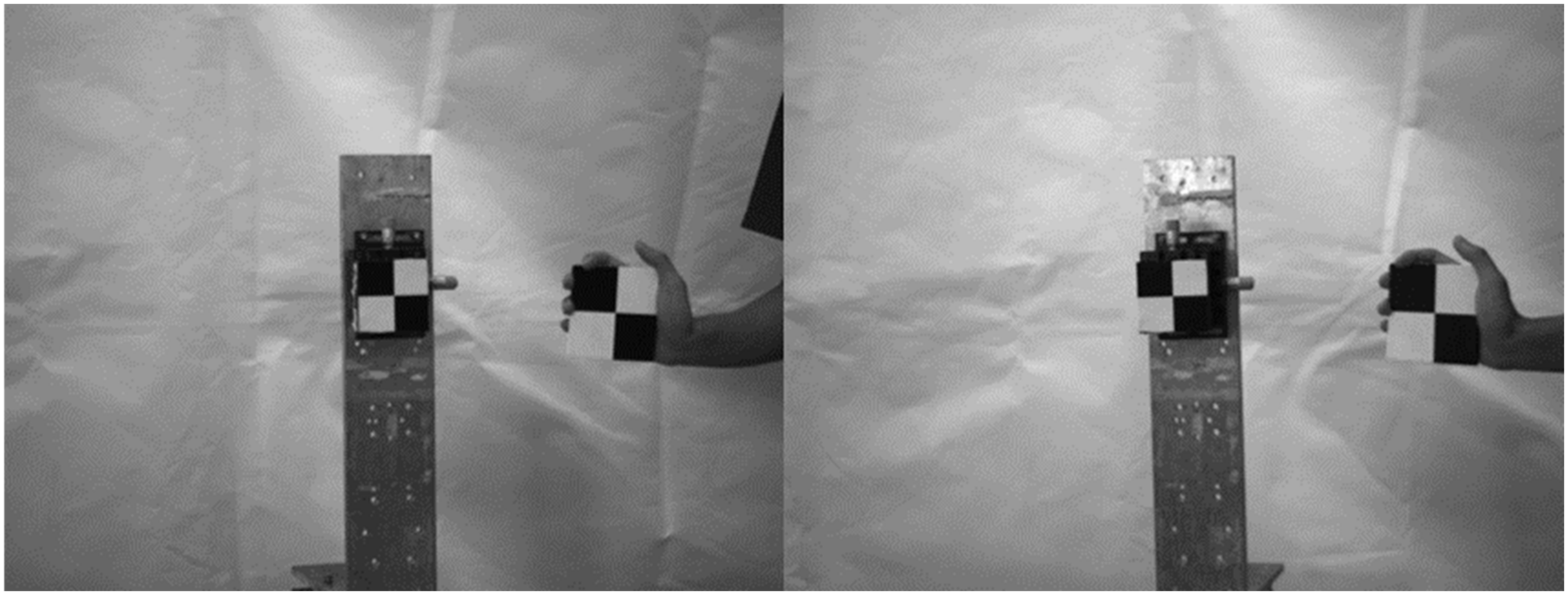
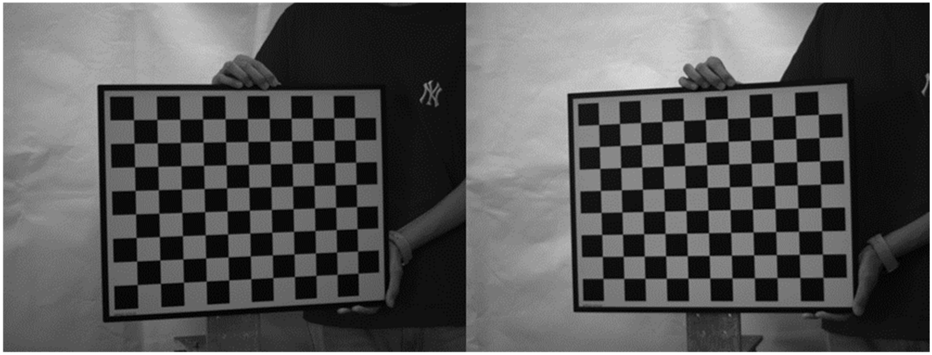
3.2.1. Experimental Procedure
3.2.2. Experimental Results
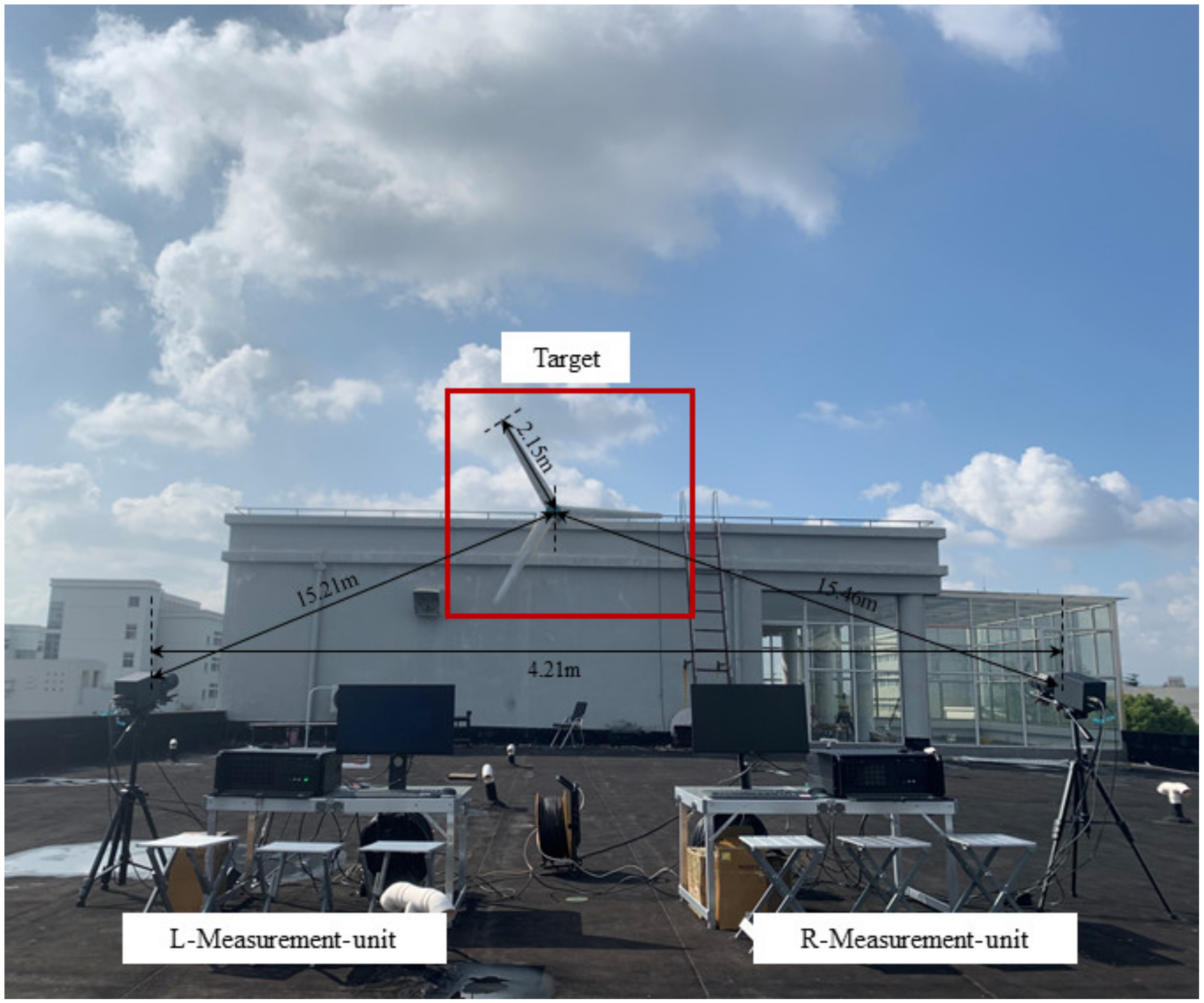
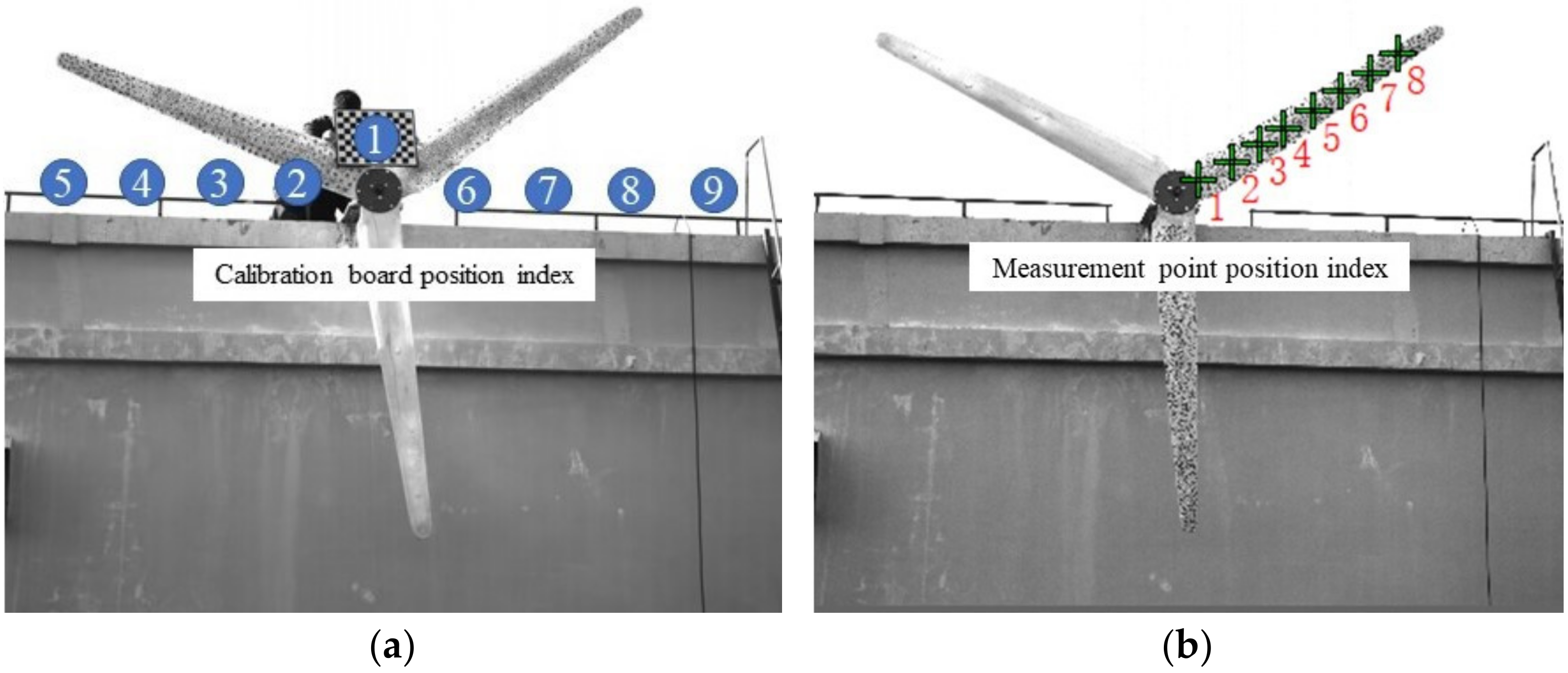
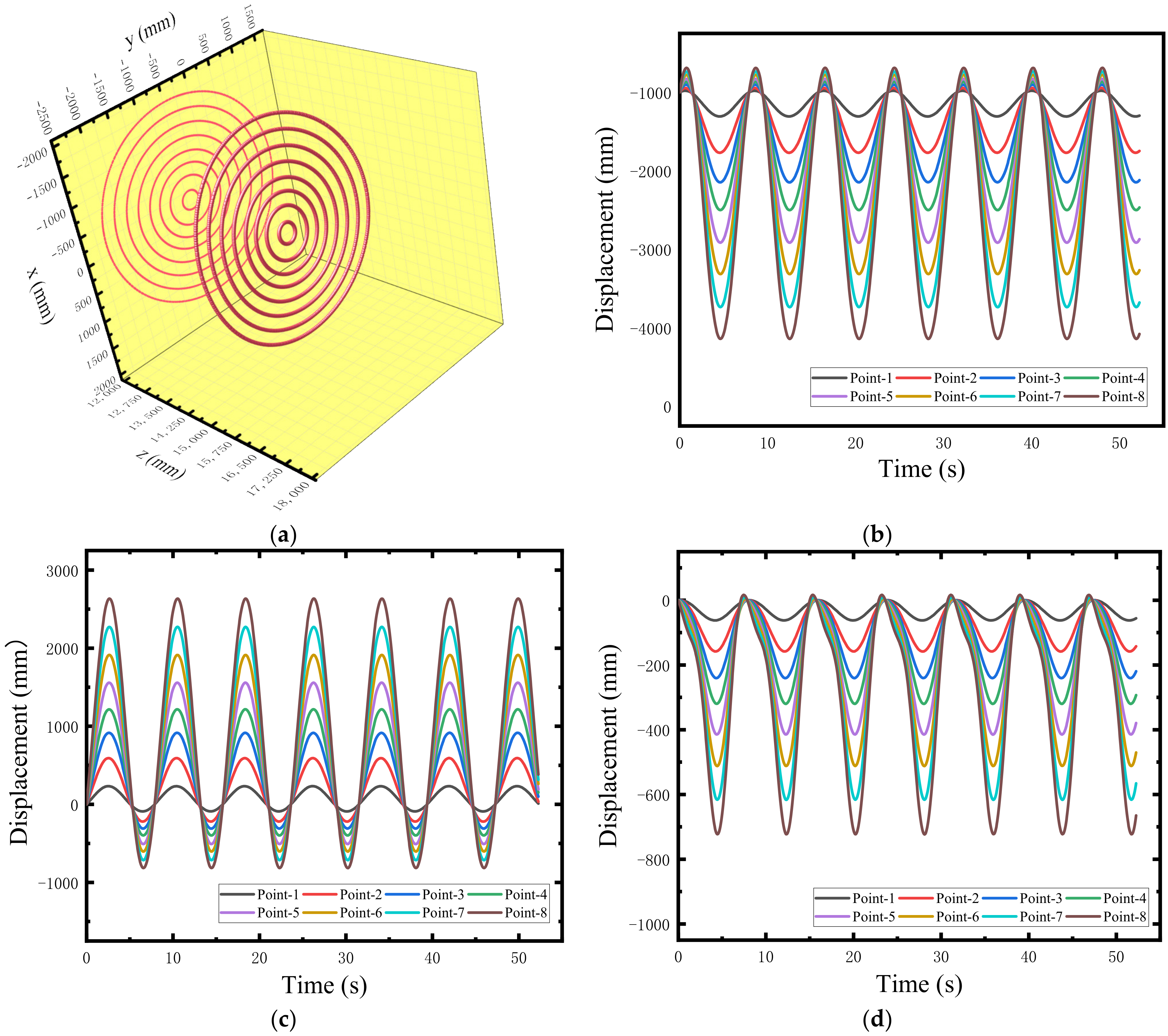
3.3. Outdoor Large FOV Experiment
3.3.1. Experimental Setup
3.3.2. Experimental Results
4. Discussion
5. Conclusions
Author Contributions
Funding
Data Availability Statement
Conflicts of Interest
References
- Zhang, S.; Mao, S.; Arola, D.; Zhang, D. Characterization of the strain-life fatigue properties of thin sheet metal using an optical extensometer. Opt. Lasers Eng. 2014, 60, 44–48. [Google Scholar] [CrossRef]
- Su, Z.; Pan, J.; Zhang, S.; Wu, S.; Yu, Q.; Zhang, D. Characterizing dynamic deformation of marine propeller blades with stroboscopic stereo digital image correlation. Mech. Syst. Signal Process. 2022, 162, 108072. [Google Scholar] [CrossRef]
- Brown, D. Close-Range Camera Calibration. Photogramm. Eng. 2002, 37, 855–866. [Google Scholar]
- Luhmann, T.; Fraser, C.; Maas, H.-G. Sensor modelling and camera calibration for close-range photogrammetry. ISPRS J. Photogramm. Remote Sens. 2016, 115, 37–46. [Google Scholar] [CrossRef]
- Tsai, R. A versatile camera calibration technique for high-accuracy 3D machine vision metrology using off-the-shelf TV cameras and lenses. IEEE J. Robot. Autom. 1987, 3, 323–344. [Google Scholar] [CrossRef]
- Zhang, Z. A flexible new technique for camera calibration. IEEE Trans. Pattern Anal. Mach. Intell. 2000, 22, 1330–1334. [Google Scholar] [CrossRef]
- Faugeras, O.D.; Luong, Q.T.; Maybank, S.J. Camera self-calibration: Theory and experiments. In Proceedings of the Computer Vision—ECCV’92, Berlin/Heidelberg, Germany, 19–22 May 1992; pp. 321–334. [Google Scholar]
- Brückner, M.; Bajramovic, F.; Denzler, J. Intrinsic and extrinsic active self-calibration of multi-camera systems. Mach. Vis. Appl. 2014, 25, 389–403. [Google Scholar] [CrossRef]
- Yamazaki, S.; Mochimaru, M.; Kanade, T. Simultaneous self-calibration of a projector and a camera using structured light. In Proceedings of the CVPR 2011 WORKSHOPS, Colorado Springs, CO, USA, 20–25 June 2011; pp. 60–67. [Google Scholar]
- Li, C.; Su, R. A Novel Stratified Self-calibration Method of Camera Based on Rotation Movement. J. Softw. 2014, 9, 1281–1287. [Google Scholar] [CrossRef]
- Miyata, S.; Saito, H.; Takahashi, K.; Mikami, D.; Isogawa, M.; Kojima, A. Extrinsic Camera Calibration Without Visible Corresponding Points Using Omnidirectional Cameras. IEEE Trans. Circuits Syst. Video Technol. 2018, 28, 2210–2219. [Google Scholar] [CrossRef]
- Gao, Z.; Gao, Y.; Su, Y.; Liu, Y.; Fang, Z.; Wang, Y.; Zhang, Q. Stereo camera calibration for large field of view digital image correlation using zoom lens. Measurement 2021, 185, 109999. [Google Scholar] [CrossRef]
- Sun, J.; Liu, Q.; Liu, Z.; Zhang, G. A calibration method for stereo vision sensor with large FOV based on 1D targets. Opt. Lasers Eng. 2011, 49, 1245–1250. [Google Scholar] [CrossRef]
- Wang, Y.; Wang, X. An improved two-point calibration method for stereo vision with rotating cameras in large FOV. J. Mod. Opt. 2019, 66, 1106–1115. [Google Scholar] [CrossRef]
- Liu, Z.; Li, F.; Li, X.; Zhang, G. A novel and accurate calibration method for cameras with large field of view using combined small targets. Measurement 2015, 64, 1–16. [Google Scholar] [CrossRef]
- Zhang, Y.; Liu, W.; Wang, F.; Lu, Y.; Wang, W.; Yang, F.; Jia, Z. Improved separated-parameter calibration method for binocular vision measurements with a large field of view. Opt. Express 2020, 28, 2956–2974. [Google Scholar] [CrossRef]
- Gorjup, D.; Slavič, J.; Boltežar, M. Frequency domain triangulation for full-field 3D operating-deflection-shape identification. Mech. Syst. Signal Process. 2019, 133, 106287. [Google Scholar] [CrossRef]
- Poozesh, P.; Sabato, A.; Sarrafi, A.; Niezrecki, C.; Avitabile, P.; Yarala, R. Multicamera measurement system to evaluate the dynamic response of utility-scale wind turbine blades. Wind Energy 2020, 23, 1619–1639. [Google Scholar] [CrossRef]
- Jiang, T.; Cui, H.; Cheng, X. A calibration strategy for vision-guided robot assembly system of large cabin. Measurement 2020, 163, 107991. [Google Scholar] [CrossRef]
- Nister, D. An efficient solution to the five-point relative pose problem. IEEE Trans. Pattern Anal. Mach. Intell. 2004, 26, 756–770. [Google Scholar] [CrossRef] [PubMed]
- Hartley, R.I. In defense of the eight-point algorithm. IEEE Trans. Pattern Anal. Mach. Intell. 1997, 19, 580–593. [Google Scholar] [CrossRef]
- Fathian, K.; Gans, N.R. A new approach for solving the Five-Point Relative Pose Problem for vision-based estimation and control. In Proceedings of the 2014 American Control Conference, Portland, OR, USA, 2014, 4–6 June 2014; pp. 103–109. [Google Scholar]
- Feng, W.; Su, Z.; Han, Y.; Liu, H.; Yu, Q.; Liu, S.; Zhang, D. Inertial measurement unit aided extrinsic parameters calibration for stereo vision systems. Opt. Lasers Eng. 2020, 134, 106252. [Google Scholar] [CrossRef]
- D’Alfonso, L.; Garone, E.; Muraca, P.; Pugliese, P. On the use of the inclinometers in the PnP problem. In Proceedings of the 2013 European Control Conference (ECC), Zurich, Switzerland, 17–19 July 2013; pp. 4112–4117. [Google Scholar]
- Zhang, D.; Yu, Z.; Xu, Y.; Ding, L.; Ding, H.; Yu, Q.; Su, Z. GNSS Aided Long-Range 3D Displacement Sensing for High-Rise Structures with Two Non-Overlapping Cameras. Remote Sens. 2022, 14, 379. [Google Scholar] [CrossRef]
- Shi, J.; Tomasi, C. Good features to track. In Proceedings of the 1994 IEEE Conference on Computer Vision and Pattern Recognition, Seattle, WA, USA, 21–23 June 1994; pp. 593–600. [Google Scholar]
- Feng, W.; Zhang, S.; Liu, H.; Yu, Q.; Wu, S.; Zhang, D. Unmanned aerial vehicle-aided stereo camera calibration for outdoor applications. Opt. Eng. 2020, 59, 014110. [Google Scholar] [CrossRef]
- Yang, D.; Su, Z.; Shuiqiang, Z.; Zhang, D. Real-time Matching Strategy for RotaryObjects using Digital Image Correlation. Appl. Opt. 2020, 59, 6648–6657. [Google Scholar] [CrossRef] [PubMed]


| Intrinsic Parameters | Left Camera | Right Camera |
|---|---|---|
| (pixels) | 8701.27 | 8715.25 |
| (pixels) | 8697.10 | 8713.49 |
| (pixels) | 2003.92 | 1970.53 |
| (pixels) | 1447.46 | 1477.75 |
| −0.091 | −0.153 | |
| −0.006 | 2.694 |
| Extrinsic Parameters | Proposed Method | Zhang’s Method |
|---|---|---|
| Rotation vector (°) | (−0.46, 29.36, −0.37) | (−0.27, 29.32, −0.56) |
| Translation vector (mm) | (−857.10, −10.63, 255.27) | (−854.80, −9.49, 259.81) |
| Translation | Proposed Method | Zhang’s Method | |||
|---|---|---|---|---|---|
| Motion | Direction | Measured | Error | Measured | Error |
| 3.500 | X | 3.509 | 0.009 | 3.514 | 0.014 |
| Y | 3.511 | 0.011 | 3.515 | 0.015 | |
| Z | 3.512 | 0.012 | 3.492 | −0.008 | |
| 7.000 | X | 6.989 | −0.011 | 7.018 | 0.018 |
| Y | 7.013 | 0.013 | 7.011 | 0.011 | |
| Z | 7.016 | 0.016 | 6.992 | −0.008 | |
| 10.500 | X | 10.508 | 0.008 | 10.507 | 0.007 |
| Y | 10.488 | −0.012 | 10.506 | 0.006 | |
| Z | 10.492 | −0.008 | 10.505 | 0.005 | |
| 14.000 | X | 14.014 | 0.014 | 14.013 | 0.013 |
| Y | 13.085 | −0.015 | 14.009 | 0.009 | |
| Z | 13.987 | −0.013 | 14.011 | 0.011 | |
| 17.500 | X | 17.509 | 0.009 | 17.013 | 0.013 |
| Y | 17.017 | 0.017 | 16.085 | −0.015 | |
| Z | 17.508 | 0.008 | 17.515 | 0.015 | |
| Mean error | 0.012 | 0.011 | |||
| Intrinsic Parameters | Left Camera | Right Camera |
|---|---|---|
| (pixels) | 15,953.42 | 16,067.16 |
| (pixels) | 15,948.73 | 16,060.78 |
| (pixels) | 2613.21 | 2471.86 |
| (pixels) | 2515.96 | 2478.96 |
| 0.042 | 0.027 | |
| −0.681 | −0.3817 |
| Extrinsic Parameters | Proposed Method | Traditional Method |
|---|---|---|
| Rotation vector (°) | (−1.31, 16.55, −1.12) | (−1.22, 16.64, −1.11) |
| Translation vector (mm) | (−4145.09, 83.75, 718.65) | (−4145.54, 106.12, 726.15) |
Disclaimer/Publisher’s Note: The statements, opinions and data contained in all publications are solely those of the individual author(s) and contributor(s) and not of MDPI and/or the editor(s). MDPI and/or the editor(s) disclaim responsibility for any injury to people or property resulting from any ideas, methods, instructions or products referred to in the content. |
© 2023 by the authors. Licensee MDPI, Basel, Switzerland. This article is an open access article distributed under the terms and conditions of the Creative Commons Attribution (CC BY) license (https://creativecommons.org/licenses/by/4.0/).
Share and Cite
Wang, J.; Guan, B.; Han, Y.; Su, Z.; Yu, Q.; Zhang, D. Sensor-Aided Calibration of Relative Extrinsic Parameters for Outdoor Stereo Vision Systems. Remote Sens. 2023, 15, 1300. https://doi.org/10.3390/rs15051300
Wang J, Guan B, Han Y, Su Z, Yu Q, Zhang D. Sensor-Aided Calibration of Relative Extrinsic Parameters for Outdoor Stereo Vision Systems. Remote Sensing. 2023; 15(5):1300. https://doi.org/10.3390/rs15051300
Chicago/Turabian StyleWang, Jing, Banglei Guan, Yongsheng Han, Zhilong Su, Qifeng Yu, and Dongsheng Zhang. 2023. "Sensor-Aided Calibration of Relative Extrinsic Parameters for Outdoor Stereo Vision Systems" Remote Sensing 15, no. 5: 1300. https://doi.org/10.3390/rs15051300
APA StyleWang, J., Guan, B., Han, Y., Su, Z., Yu, Q., & Zhang, D. (2023). Sensor-Aided Calibration of Relative Extrinsic Parameters for Outdoor Stereo Vision Systems. Remote Sensing, 15(5), 1300. https://doi.org/10.3390/rs15051300