Camouflaged Object Detection Based on Ternary Cascade Perception

Abstract

Camouflaged object detection (COD), in a broad sense, aims to detect image objects that have high degrees of similarity to the background. COD is more challenging than conventional object detection because of the high degree of “fusion” between a camouflaged object and the background. In this paper, we focused on the accurate detection of camouflaged objects, conducting an in-depth study on COD and addressing the common detection problems of high miss rates and low confidence levels. We proposed a ternary cascade perception-based method for detecting camouflaged objects and constructed a cascade perception network (CPNet). The innovation lies in the proposed ternary cascade perception module (TCPM), which focuses on extracting the relationship information between features and the spatial information of the camouflaged target and the location information of key points. In addition, a cascade aggregation pyramid (CAP) and a joint loss function have been proposed to recognize camouflaged objects accurately. We conducted comprehensive experiments on the COD10K dataset and compared our proposed approach with other seventeen-object detection models. The experimental results showed that CPNet achieves optimal results in terms of six evaluation metrics, including an average precision (AP)₅₀ that reaches 91.41, an AP₇₅ that improves to 73.04, and significantly higher detection accuracy and confidence.

1. Introduction

Camouflaged object detection (COD), in a narrow sense, aims at detecting objects hidden in image scenes [1], such as chameleons hiding in their environment via epidermal color changes [2] or armed soldiers lurking in mountains and forests. In a broader sense, COD aims at detecting any image objects with low detectability, such as component defects in the industry [3] or signs of lesions in pathology [4]. The study of COD is not only an important scientific problem in the field of computer vision but can also bring great economic and social benefits.

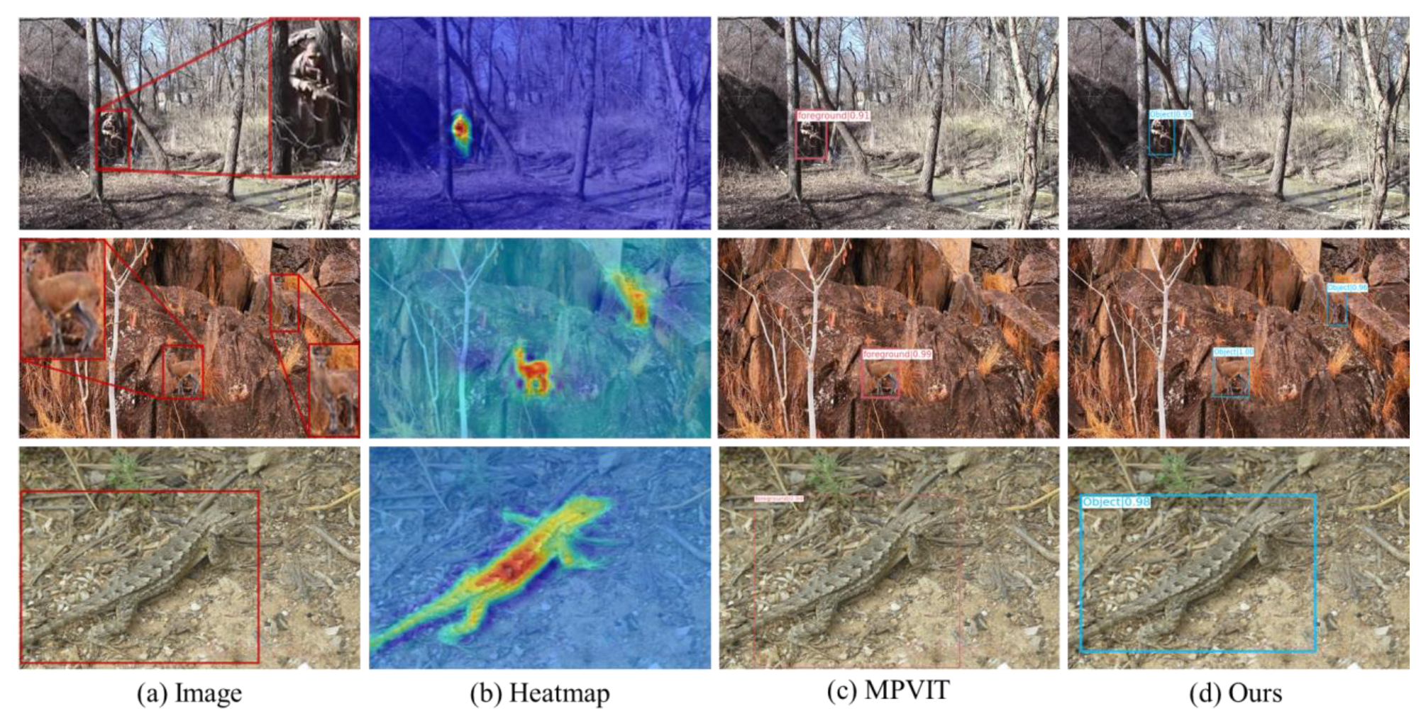
However, the colors and patterns of camouflaged objects almost blend with the environment, which greatly reduces their probability of them being detected, identified, or targeted [5]. Figure 1 shows two cases: artificial camouflage, in which soldiers wearing special camouflage clothing and who are obscured by objects can conceal themselves, and natural camouflage, where lizards and deer have evolved their bodies to resist natural enemies and hunt prey with colors similar to their environment. In both cases, they can almost perfectly achieve the effect of blending with the background.

To date, the corresponding research on camouflaged target identification has mainly focused on two aspects. The first aspect is the identification of camouflaged objects with the help of nonvisible detection techniques. Camouflaged objects can effectively hamper the detection of visible wavelengths, while the combination of detection techniques in other wavelengths, such as infrared, hyperspectral, and polarized wavelengths, can make up for the shortcomings of visible detection itself [6,7,8]; although this method is effective, it does not solve the scientific problem of detecting camouflaged targets in visible wavelengths. The second aspect is the study of COD techniques in visible wavelengths. Before the rapid development of deep learning, researchers commonly used traditional digital image processing methods, such as spectral transforms [9], sparse matrices [10], and human vision systems [11], which are not robust and have poor generalization performance. In recent years, with the development of deep learning technology, scholars have applied it to the detection of camouflaged objects, providing new ideas for the detection of camouflaged objects in visible wavelengths [12].

The current general deep learning object detection networks (e.g., the multi-path vision transformer (MPVIT) [13]) are effective for detecting salient objects in images, but as shown in Figure 1, they often produce missed detections and low confidence when detecting camouflaged objects for the following three reasons:

• The color and texture are highly similar between the camouflaged object and the background and reduce the differences in their features.
• Camouflaged objects usually have irregular shapes and varying scales, making the spatial information of these objects in images extremely complex.
• The low utilization of the highly representative key point information of the camouflaged objects results in missed detections and false alarms.

This paper proposed a ternary cascade perception-based method for detecting camouflaged objects to solve the abovementioned problems. The innovative feature is the ternary cascade perception module (TCPM), which focuses on extracting the relationship information between features, the spatial information of camouflaged targets, and the location information of key points. Second, we improved the existing feature fusion module and proposed a cascade aggregation pyramid (CAP) to achieve more efficient feature fusion. Finally, we proposed a joint loss function, which used multiple loss functions for the prediction of target classes and bounding boxes and jointly obtained the training loss values.

The main contributions of this paper are as follows:

• To overcome the deficiencies of existing COD methods, the TCPM was proposed to solve the problems of missed detections and low confidence levels.
• Combined with the TCPM, a cascade perception-based COD network (CPNet) was constructed, and a designed CAP with a joint loss function was also used in the network to make it more targeted for COD.
• The proposed CPNet demonstrated the best performance on the COD10K camouflaged object dataset, and all the metrics were better than or on par with the published methods.

The rest of this paper is structured as follows: In Section 2, we introduced the related work. In Section 3, we introduced the network structure of CPNet in detail. Section 4 gives the discussions of experimental results. Finally, we summarized the research content in Section 5.

2. Related Work

This section mainly compares the deep learning-based camouflaged object recognition methods and generic object detection methods that are relevant to this work.

2.1. Generic Object Detection Based on Deep Learning

Object detection is a subtask of object recognition that aims to detect the presence of predefined objects in an image and localizes them by bounding box annotations. Currently, two-step detection algorithms and one-step detection algorithms are available [14]. Two-step detection algorithms mainly include the fast region-based convolutional neural network (RCNN) [15], Mask RCNN [16], and DetectoRS [17], whose main aim is first to generate candidate regions and then perform classification and detection on the regions; these approaches are more accurate than other approaches. One-step detection algorithms mainly include you only look once (YOLO) [18], CenterNet [19], and EfficientDet [20]. These algorithms adopt the end-to-end idea without extracting candidate regions and employ grid partitioning to complete target detection in the given grid, which can achieve a reduction in the detection time. The two-step detection algorithms have been widely studied due to their high accuracy. Lee et al. used a Swin transformer network and multi-path parallelism to achieve efficient utilization of feature information [13]. Ke et al. further improved the accuracy of the two-step detection algorithm by searching for poor-quality regions through quadtrees [21]. The aim of this work is camouflage object detection, which is often difficult to detect due to its special characteristics. Therefore, this research followed the idea of two-step detection algorithms in order to make the network as accurate as possible. In recent years, researchers have proposed many methods to improve accuracy (e.g., contextual information aggregation [22], multi-scale detection [23], and feature information reweighting [24]). This has facilitated the use of deep learning-based target detection techniques in a wide range of applications, such as aerial detection [25,26] unmanned vehicles [27], and geological exploration [28,29].

2.2. Camouflaged Object Recognition Based on Deep Learning

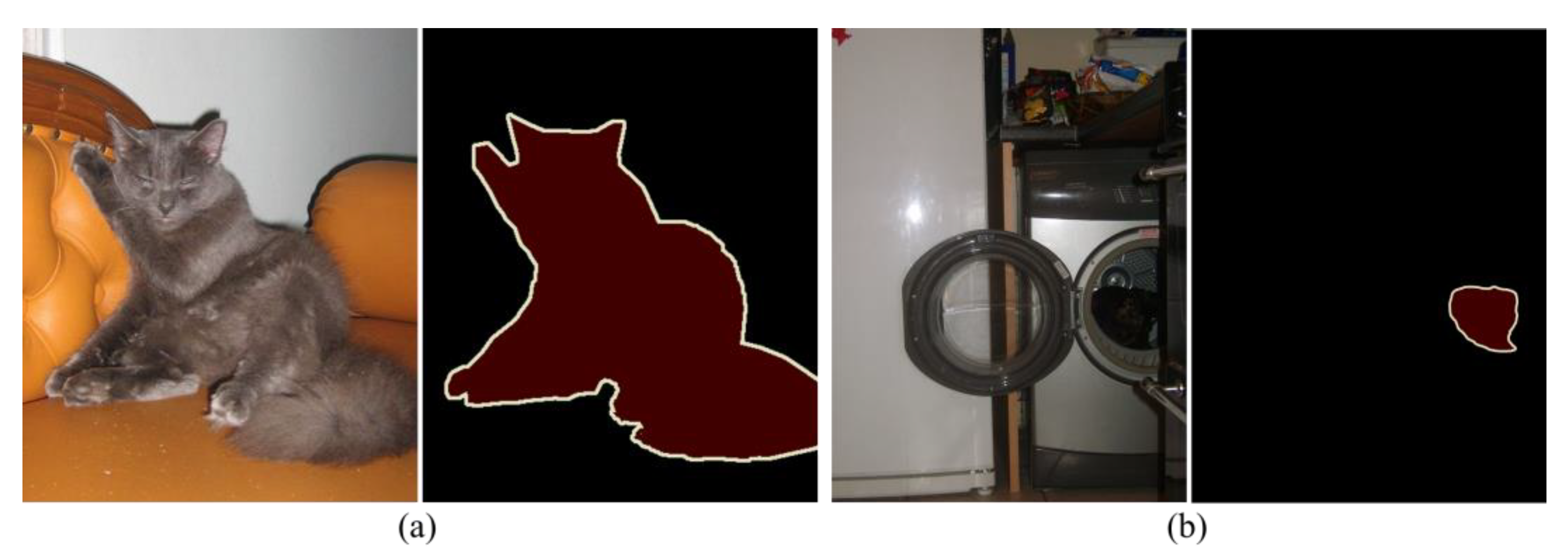
Figure 2 shows the difference between a camouflaged object and a generic object. Both pictures are marked with cats, (a) taken from the general object dataset PASCAL VOC and (b) taken from the COD dataset COD10K. As can be seen, COD is more difficult than SOD. In the introduction, we also discussed that generic object detection networks usually lack the ability to detect camouflaged objects. In recent years, deep learning techniques have advanced abruptly, and scholars have applied them to the field of camouflage object recognition. In 2020, Fan et al. established a universal camouflaged object dataset called COD10K, which has promoted the accelerated application of deep-learning-based camouflaged object recognition approaches [30]. In 2021, Mei et al. proposed a camouflaged object recognition network called the positioning and focus network (PFNet) based on the principle of distraction mining to simulate animal predation in nature [31]. Jiang et al. also proposed a camouflaged object segmentation network called the magnifier network (MAGNet) based on a simulated magnifying glass observation effect with the help of the bionic principle [32]. In the same year, Lv et al. proposed a new camouflaged object segmentation dataset called NC4K and proposed a network that can simultaneously perform localization, segmentation, and camouflage effect ranking [33]. In 2022, Pang et al. proposed a mixed-scale triadic model called the zoom-in and -out network (ZoomNet) by mimicking the human behavior of zooming in and out when observing blurred images; this is the state-of-the-art model in the field of camouflaged target segmentation [34].

As mentioned above, most of the existing research on deep learning-based camouflaged object recognition has focused on pixel-level segmentation, and the segmentation networks are often complex and time-consuming. In practice, some applications of camouflaged object detection (e.g., intrusion detection [35], military target recognition [36]) often do not require extremely accurate segmentation but only need to detect the presence of the target; therefore, this paper focused on camouflaged object detection rather than pixel-level segmentation.

3. Methods

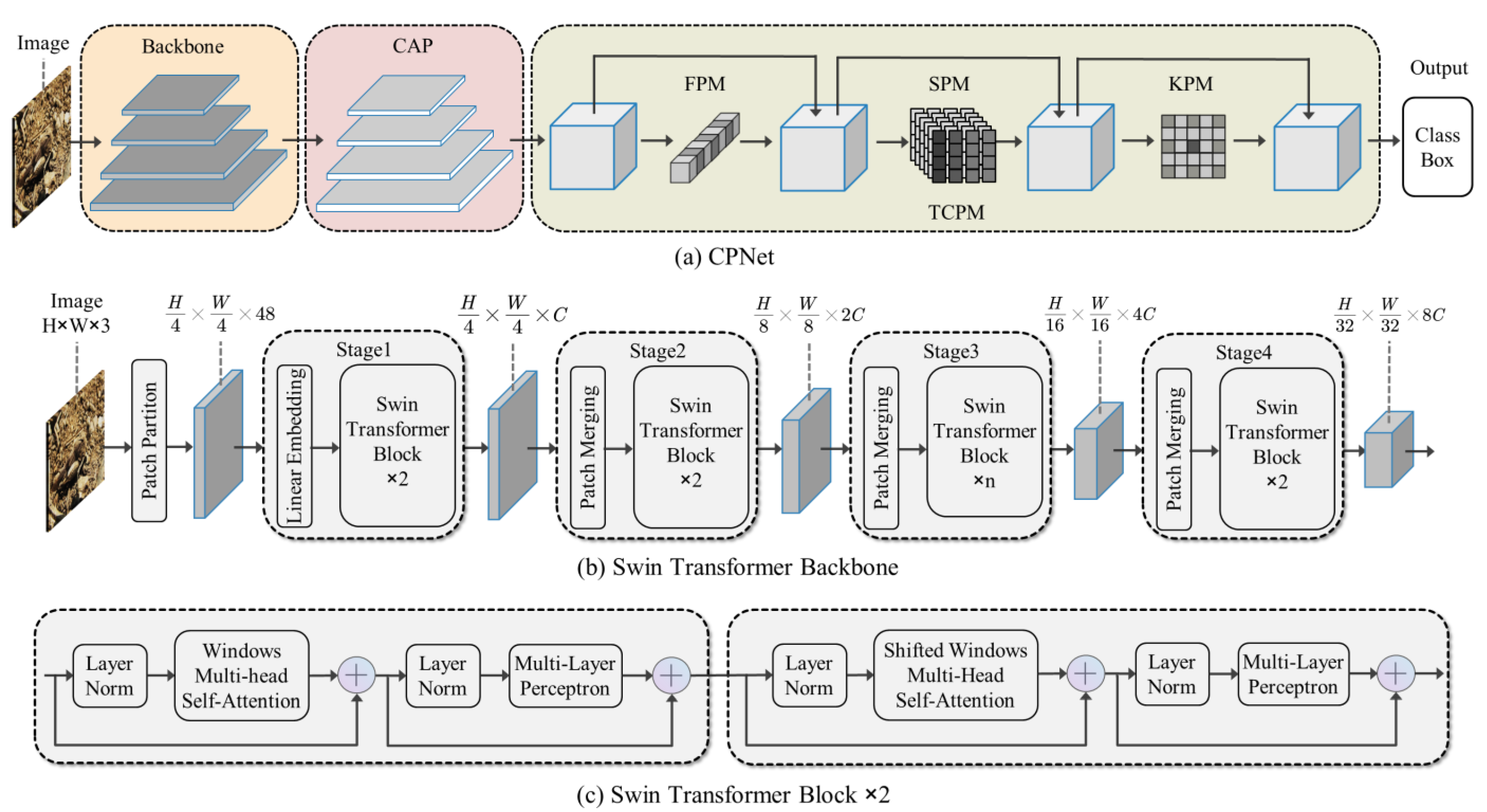
The structure of the proposed CPNet for COD is shown in Figure 3a. The CPNet sequentially cascades the feature extraction backbone, the CAP, the TCPM, and the detection output head. The feature extraction backbone downsamples the input image to 1/4, 1/8, 1/16, and 1/32 of the original size and then inputs the four sets of feature maps into the CAP for feature fusion. The CAP outputs four 3D tensors, which are then fed into the TCPM for information perception, and the object class and object bounding box information is finally output.

The design ideas and specific structures of each component will be discussed in detail below.

3.1. Feature Extraction Backbone

The feature extraction backbone (Backbone) was used to extract the feature information at each scale in the input image. For the multi-scale phenomenon of camouflaged objects, the Swin transformer feature extraction network [37] with good comprehensive performance was used, and its structure is shown in Figure 3b. The Swin transformer draws on the layered sliding window structure of traditional CNNs. First, the image to be recognized in the input network is partitioned into patches; adjacent 4 × 4 pixels constitute a patch, and each patch is mapped to superpixel points. The number of output channels is 4 × 4 × 3. The output of this step is ${\mathcal{F}}_{pp}\in {\mathcal{R}}^{\frac{W}{4}\times \frac{H}{4}\times 48}$. Then, the Swin transformer performs downsampling by merging the patches and obtaining multi-scale feature representations. Each stage extracts features through the sliding window of the Swin transformer block and detects low-level features and high-level features. The Swin transformer block is shown in Figure 3c. Finally, the generated feature maps during each stage are input into the CAP. The Swin transformer backbones with different sizes have different numbers of Swin transformer blocks n and the number of channels C. The Swin transformer models with larger n and C have better classification accuracy on the ImageNet dataset [38]. CPNet selected two models, Swin-T and Swin-S, for the experiment.

Table 1. Swin transformer backbone specifications.

Backbone	Input Size	Number of Blocks	Number of Channels	Params (M)	FLOPs (G)	Top-1 Acc (%)
Swin-T	2242	6	96	27.50	4.36	81.3
Swin-S	2242	18	96	48.79	8.52	83.0

shows the parameter settings of the Swin transformer backbone and the experimental results obtained on the standard classification dataset (ImageNet-1K).

3.2. CAP

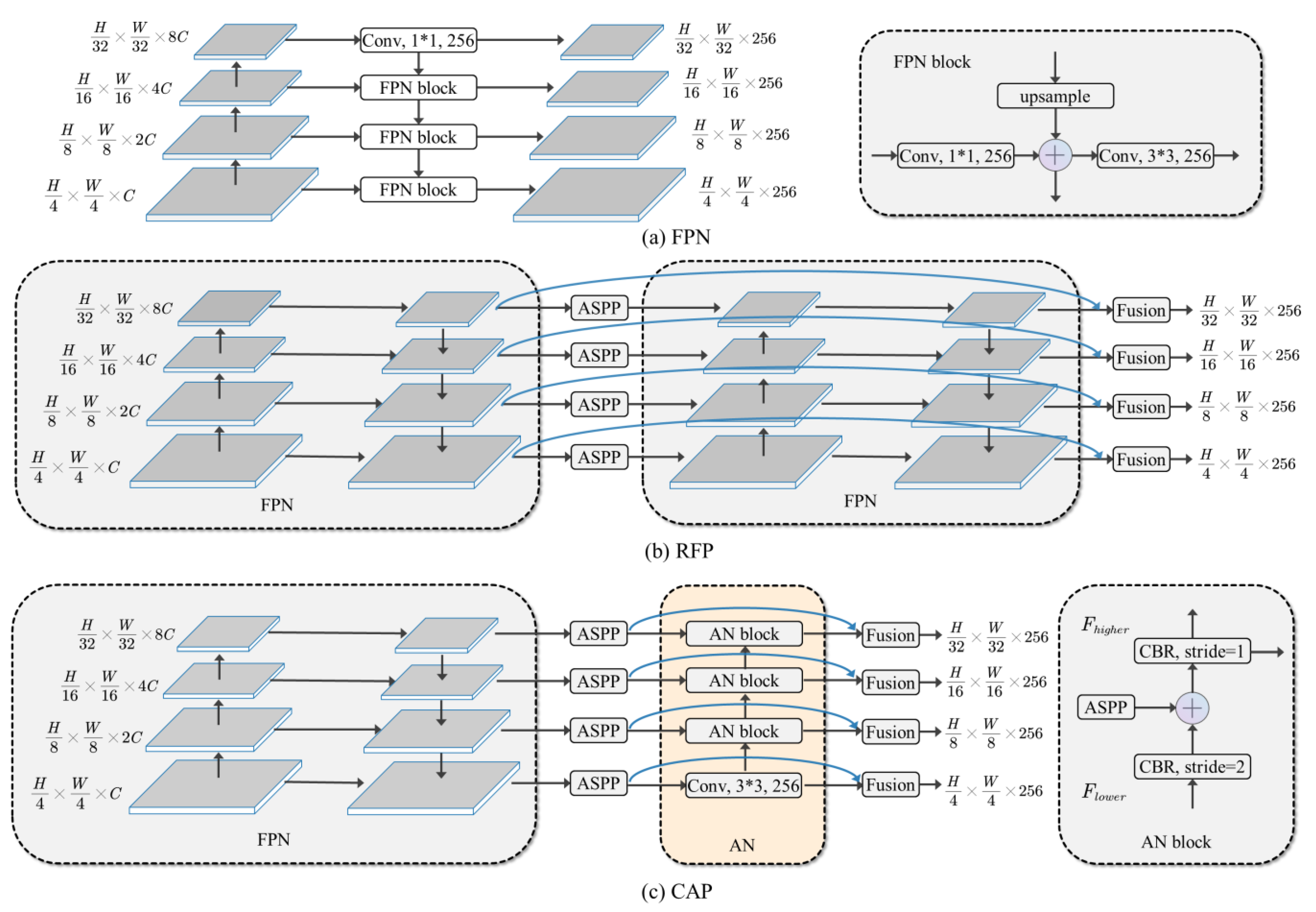
In the feature extraction network, the low-level feature map contains a large amount of location information, while the high-level feature map carries stronger semantic information after continuous feature extraction. In 2021, Qiao et al. proposed the recursive feature pyramid (RFP) [17], a module that improves upon the feature pyramid network (FPN) [39] by adopting the design idea of “looking and thinking twice” to feed the feature maps from the primary training step of the FPN into the backbone network for fusing the information between the high- and low-level features several times, while achieving enhanced semantic representation and target localization. The FPN structure is shown in Figure 4a, and the RFP structure is shown in Figure 4b. The receptive field of the first output feature map FPN in RFP was firstly enhanced by using atrous spatial pyramid pooling (ASPP) [40], and then the feature extraction and feature fusion were performed again using FPN. Finally, the two sets of feature maps were fused to achieve a stronger representation.

The RFP makes the model training time and inference time too long due to its complex structure and multiple training of the backbone. In this paper, the RFP was improved in a targeted way for efficient object detection, called the CAP, as shown in Figure 4c.

The CAP changed the secondary training part of the RFP to an aggregation network (AN). First, the lower-level feature map ${\mathcal{F}}_{lower}$ is downsampled using the convolutional layer combination of convolution + batch normalization + Relu activation function (CBR) with a step size of 2. It aggregates low-level representations and obtains higher-lever ${\mathcal{F}}_{CBR}$:

$${\mathcal{F}}_{CBR}=Conv(BN(Relu({\mathcal{F}}_{lower}))),$$

(1)

where $Conv(BN(Relu(·)))$ denotes the execution of the convolutional layer. Then, the feature maps ${\mathcal{F}}_{ASPP}$ output from the primary training part with receptive field enhancement are added together, and finally, the fusion between the feature maps is performed using the CBR with a step size of 1 to obtain higher-level features ${\mathcal{F}}_{higher}$.

$${\mathcal{F}}_{higher}=Conv(BN(Relu({\mathcal{F}}_{CBR}+{\mathcal{F}}_{ASPP}))).$$

(2)

The feature fusion from high-level representation to low-level presentation in CAP is implemented by the FPN block in FPN, and the feature aggregation from low-level presentation to high-level representation is implemented by the AN block. The AN block enhances the low-level location features by aggregating them with multiple CBR steps, which further improves the localization capability of the network. After fusing features by CAP, a multi-scale feature map containing both location and semantic information can be obtained.

3.3. TCPM

To accurately detect a camouflaged object in an image and solve the problem that the key information of the camouflaged object is difficult to obtain, the TCPM was purposely constructed. It focuses on extracting the relationship information between features, the spatial information of the camouflaged object, and the location information of key points.

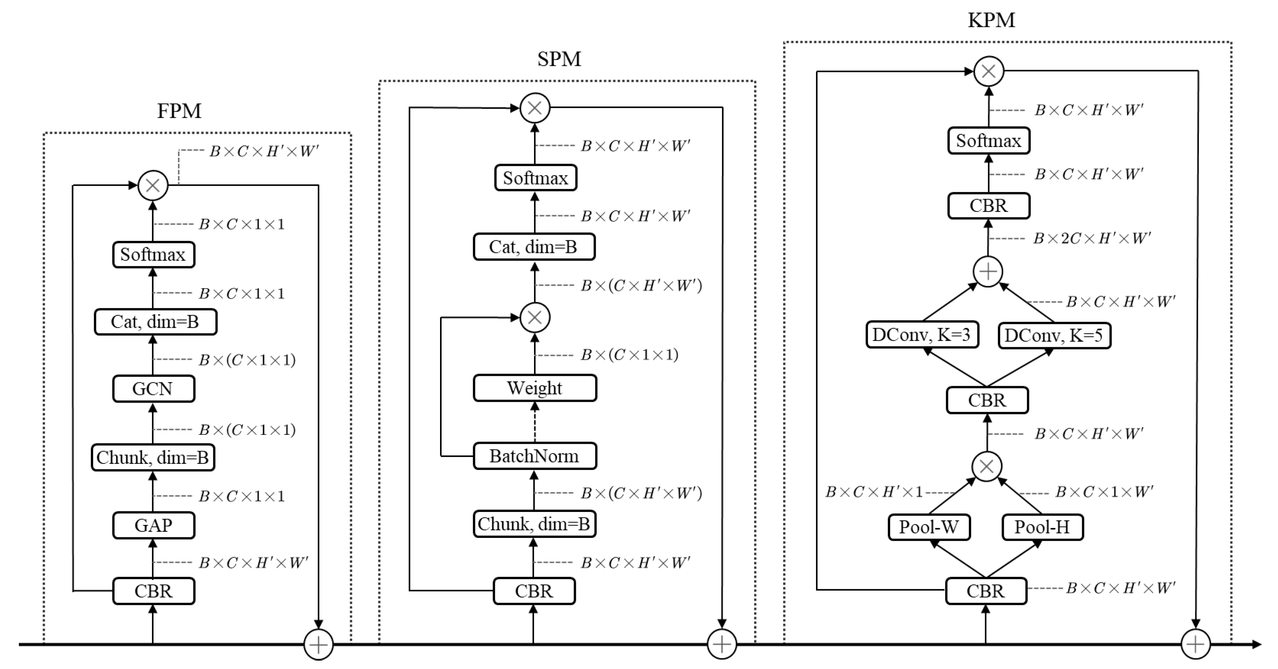
The TCPM was built based on the characteristics of camouflaged objects, and it includes a feature perception module (FPM), a spatial perception module (SPM), and a key point perception module (KPM), which are embedded into the network in a cascaded manner. The structure of the TCPM is shown in Figure 5.

3.3.1. FPM

The FPM uses a graph convolution network (GCN) [41] to obtain information regarding the relative relationships between adjacent features, thus increasing the variance of the features and making the network more capable of distinguishing mismatched content from the background.

The input tensor $\mathcal{F}\in {\mathcal{R}}^{B\times C\times H^{\prime }\times W^{\prime }}$ is preprocessed using the convolutional layer combination (CBR) to obtain the feature map ${\mathcal{F}}_{CBR}^{FPM}\in {\mathcal{R}}^{B\times C\times H^{\prime }\times W^{\prime }}$:

$${\mathcal{F}}_{CBR}^{FPM}=Conv(BN(Relu(\mathcal{F}))).$$

(3)

Second, the entire feature map is bidimensionally pooled by global average pooling (GAP) to generate a pooled feature map ${\mathcal{F}}_{GAP}\in {\mathcal{R}}^{B\times C\times 1\times 1}$:

$${\mathcal{F}}_{GAP}=GAP({\mathcal{F}}_{CBR}^{FPM},(W=1,H=1)),$$

(4)

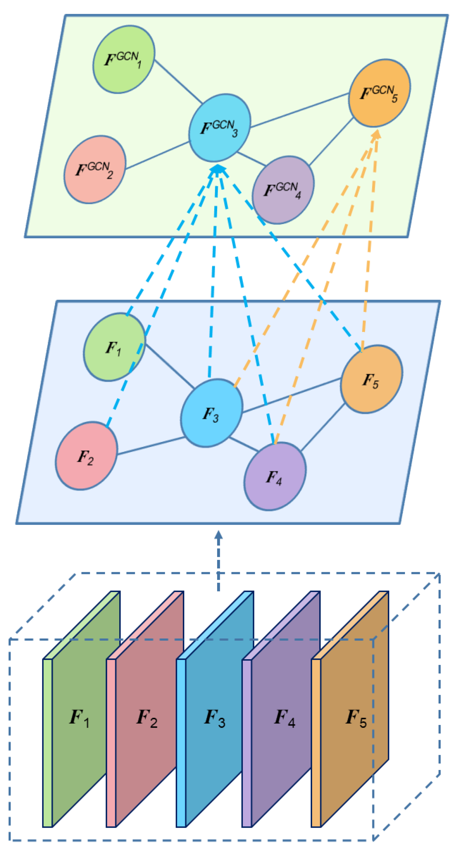
where $GAP(·,(W=1,H=1))$ represents the operation of the global average pooling the input feature map into a feature map with W = 1 and H = 1. Then, the four-dimensional tensor output of GAP is truncated into B three-dimensional tensors. In the CNN, the number of channels C represents the number of features extracted from the feature map, so the B three-dimensional tensors can be considered as a point set of C features. The GCN (a CNN that is capable of obtaining relationship information) is used to further obtain the relative relationship between the feature nodes. Its schematic is shown in Figure 6. Suppose there are five feature tensors $F_1$–$F_5$, which are regarded as five nodes, and each node carries its neighbor information by GCN (for example, $F_5$ carries the information of the 2 nodes adjacent to it to form $F^{GC{N}_5}$ after the GCN).

After obtaining the new 3D feature map tensor ${\mathcal{F}}_{GCN}\in {\mathcal{R}}^{B\times (C\times 1\times 1)}$ with node relationships, the 3D tensor is connected. Then, the softmax is performed on the channel dimension to normalize the relationship information and obtain the weight factor feature map ${\mathcal{F}}_{Weight}^{FPM}\in {\mathcal{R}}^{B\times C\times 1\times 1}$:

$$\begin{gathered} {\mathcal{F}}_{Weight}^{FPM}=Softmax(Cat(GCN({\mathcal{F}}_{GAP})),\dim =\mathrm{C}) \\ =\frac{\exp (Cat{(GCN({\mathcal{F}}_{GAP}))}_{B,i,1,1})}{{\displaystyle \sum _{0\le i<C}\exp (Cat{(GCN({\mathcal{F}}_{GAP}))}_{B,i,1,1})}} \end{gathered}$$

(5)

where $Softmax(·,\dim =\mathrm{C})$ denotes the softmax operation on the channel dimension. The weight factor feature map ${\mathcal{F}}_{Weight}^{FPM}$ is multiplied with the preprocessed feature map ${\mathcal{F}}_{CBR}^{FPM}$ channel by channel to obtain the relationship-weighted feature map ${\mathcal{F}}_{Weighted}^{FPM}\in {\mathcal{R}}^{B\times C\times H^{\prime }\times W^{\prime }}$. Finally, ${\mathcal{F}}_{Weighted}^{FPM}$ is connected with the original input for the residuals and added pixel-by-pixel to obtain the output feature tensor ${\mathcal{F}}_{Output}^{FPM}\in {\mathcal{R}}^{B\times C\times H^{\prime }\times W^{\prime }}$ of the FPM, which is reinput into the main network.

$${\mathcal{F}}_{Output}^{FPM}={\mathcal{F}}_{Weighted}^{FPM}\oplus \mathcal{F}=({\mathcal{F}}_{CBR}^{FPM}\otimes {\mathcal{F}}_{Weight}^{FPM})\oplus \mathcal{F}.$$

(6)

3.3.2. SPM

The SPM obtains critical features through spatial normalization, which mitigates the problems of missed detections and multitarget detection by using spatial information.

For the output tensor ${\mathcal{F}}_{Output}^{FPM}\in {\mathcal{R}}^{B\times C\times H^{\prime }\times W^{\prime }}$ of the FPM, preprocessing is first performed using the convolutional layer combination (CBR) to obtain the feature map ${\mathcal{F}}_{CBR}^{SPM}\in {\mathcal{R}}^{B\times C\times H^{\prime }\times W^{\prime }}$:

$${\mathcal{F}}_{CBR}^{SPM}=Conv(BN(Relu({\mathcal{F}}_{Output}^{FPM}))).$$

(7)

The SPM improves the existing batch normalization method to obtain the spatial feature weights. Batch normalization is performed for the same channel of different feature maps within each batch, and this calculation method can utilize the semantic information of different feature maps. The literature [42] experimentally demonstrated that BN generates large errors in small batches. In addition, the category and environment gaps between different images in the camouflaged object dataset are large, the semantic information of the images input within the same batch is often not rich, and a uniform weight calculation will make the results unstable and equivalent to the introduction of noisy data into a single image. Therefore, the four-dimensional tensor ${\mathcal{F}}_{CBR}^{SPM}$ is first divided into B three-dimensional tensors and then batch normalized along the dimension. Figure 7 shows the schematic diagram of the improved batch normalization method. Different feature maps within each batch are spatially normalized along the channel direction, which can ensure that the weight calculation is performed only within the individual feature map and is not affected by the rest of the feature maps within the batch. Finally, ${\mathcal{F}}_{BN}^{SPM}\in {\mathcal{R}}^{B\times (C\times H^{\prime }\times W^{\prime })}$ is obtained after normalization.

In addition, the normalization operation trains a scale factor $\gamma$ of each channel and measures the variance within a single channel. To calculate the feature weights of the spatial dimension and indicate the importance of the channel information, each channel is assigned weights $W\gamma \in {\mathcal{R}}^{B\times (C\times 1\times 1)}$:

$$W\gamma =\frac{{\gamma }_i}{{\displaystyle {\sum }_{j=0}^C{\gamma }_j}}.$$

(8)

After fusing the weights with the feature, ${\mathcal{F}}_{W\gamma }^{SPM}\in {\mathcal{R}}^{B\times C\times H^{\prime }\times W^{\prime }}$ is obtained by

$${\mathcal{F}}_{W\gamma }^{SPM}={\mathcal{F}}_{BN}^{SPM}\otimes W\gamma .$$

(9)

Then, the B three-dimensional tensors are concatenated (cat), and a softmax normalization operation is performed on the channel dimension that normalizes the spatial information to 0~1. The weight factor feature map ${\mathcal{F}}_{Weight}^{SPM}\in {\mathcal{R}}^{B\times C\times H^{\prime }\times W^{\prime }}$ is obtained by

$$\begin{gathered} {\mathcal{F}}_{Weight}^{SPM}=Softmax(Cat({\mathcal{F}}_{W\gamma }^{SPM}),\dim =\mathrm{C}) \\ =\frac{\exp (Cat{({\mathcal{F}}_{W\gamma }^{SPM})}_{B,i,H^{\prime },W^{\prime }})}{{\displaystyle \sum _{0\le i<C}\exp (Cat{({\mathcal{F}}_{W\gamma }^{SPM})}_{B,i,H^{\prime },W^{\prime }})}} \end{gathered}$$

(10)

The weight factor feature map ${\mathcal{F}}_{Weight}^{SPM}$ is multiplied with the preprocessed feature map ${\mathcal{F}}_{CBR}^{SPM}$ and yields the spatial attention-weighted feature map ${\mathcal{F}}_{Weighted}^{SPM}\in {\mathcal{R}}^{B\times C\times H^{\prime }\times W^{\prime }}$, which is finally connected with the original input. The output feature tensor ${\mathcal{F}}_{Output}^{SPM}\in {\mathcal{R}}^{B\times C\times H^{\prime }\times W^{\prime }}$ of the SPM is obtained by pixel-wise addition.

$$\begin{gathered} {\mathcal{F}}_{Output}^{SPM}={\mathcal{F}}_{Weighted}^{SPM}\oplus {\mathcal{F}}_{Output}^{FPM} \\ =({\mathcal{F}}_{CBR}^{SPM}\otimes {\mathcal{F}}_{Weight}^{SPM})\oplus {\mathcal{F}}_{Output}^{FPM} \end{gathered}$$

(11)

3.3.3. KPM

The KPM performs information perception for the key points of the camouflaged object by two-dimensional average pooling (AP) and dilated convolution (DConv). Key points refer to those points that carry key information and can significantly affect the detection results. If the key point information of the camouflaged object is determined, the confidence levels of the remaining locations can be weakened, thus reducing the false alarm rate of the network. First, we obtained the location information of the key points by conducting AP in different dimensions; then, we increased the receptive field via DConvs at different scales to obtain more multi-scale information about the area around the key points.

The output tensor ${\mathcal{F}}_{Output}^{SPM}\in {\mathcal{R}}^{B\times C\times H^{\prime }\times W^{\prime }}$ of the SPM is first preprocessed using the CBR combination to obtain a feature map:

$${\mathcal{F}}_{CBR}^{KPM}=Conv(BN(Relu({\mathcal{F}}_{Output}^{SPM}))).$$

(12)

Unlike the FPM, AP does not operate on the whole feature map. As is shown in Figure 4, it is divided into two dimensions to obtain information regarding the positions of nodes in the horizontal and vertical dimensions of the feature map. Finally, a pair of 3D tensor-pooled feature maps ${\mathcal{F}}_{Pool-W}\in {\mathcal{R}}^{B\times C\times H^{\prime }\times 1}$ and ${\mathcal{F}}_{Pool-H}\in {\mathcal{R}}^{B\times C\times 1\times W^{\prime }}$ is obtained by

$${\mathcal{F}}_{Pool-W}=AP({\mathcal{F}}_{CBR}^{KPM},(W^{\prime }=1,H^{\prime }=H^{\prime })),$$

(13)

$${\mathcal{F}}_{Pool-H}=AP({\mathcal{F}}_{CBR}^{KPM},(W^{\prime }=W^{\prime },H^{\prime }=1)).$$

(14)

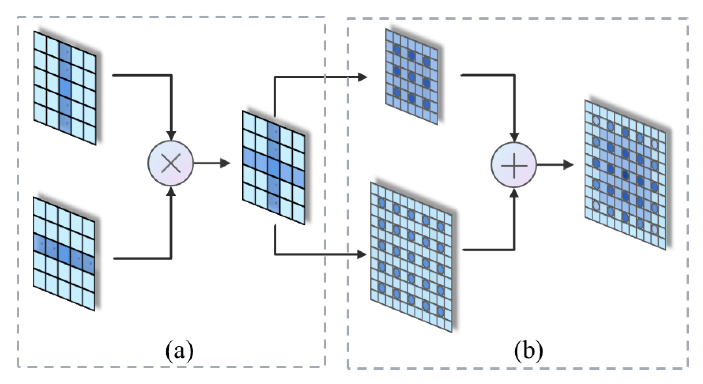
Next, the two feature maps containing the location information of the key points in different directions are multiplied (as is shown in Figure 8a) to obtain ${\mathcal{F}}_{W\times H}\in {\mathcal{R}}^{B\times C\times H^{\prime }\times W^{\prime }}$; then, the CBR combination is used to fuse the information between the channels to obtain the feature map ${\mathcal{F}}_{Location}\in {\mathcal{R}}^{B\times C\times H^{\prime }\times W^{\prime }}$ with the global location information of the embedded key points.

Local information is not enough. To accurately identify the key points of the camouflaged object, information near the key points are needed for further discrimination. For this purpose, a small feature extraction range is required for the larger location information feature map ${\mathcal{F}}_{Location}\in {\mathcal{R}}^{B\times C\times H^{\prime }\times W^{\prime }}$. Two DConv branches of different sizes are used to expand the receptive field and obtain multi-scale regional information; the schematic diagram is shown in Figure 8b with DConv kernel sizes of 3 × 3 and 5 × 5 and dilated coefficients of 2. The two sets of feature maps are superimposed to obtain a receptive field-enhanced feature map ${\mathcal{F}}_{RF}\in {\mathcal{R}}^{B\times 2C\times H^{\prime }\times W^{\prime }}$ with twice the number of channels:

$$\begin{array}{c}{\mathcal{F}}_{RF}=Add(DConv({\mathcal{F}}_{Local},K=3,D=2),\\ DConv({\mathcal{F}}_{Local},K=5,D=2))\end{array}$$

(15)

where $DConv(·,K=i,D=2)$ denotes DConv with a dilation coefficient of 2 and a convolutional kernel size of i. $Add(·,·)$ denotes the addition operation executed on the two sets of feature maps in the channel dimension. The softmax operation is performed in the channel dimension. The CBR combination is used for channel recovery and information fusion, followed by the softmax normalization operation in the channel dimension. Finally, the 3D multiscale information–weight factor feature map ${\mathcal{F}}_{Weight}^{KPM}\in {\mathcal{R}}^{B\times C\times H^{\prime }\times W^{\prime }}$ is obtained by

$$\begin{gathered} {\mathcal{F}}_{Weight}^{KPM}=Softmax(CBR({\mathcal{F}}_{RF}),\dim =\mathrm{C}) \\ =\frac{\exp ({(CBR({\mathcal{F}}_{RF}))}_{B,i,H^{\prime },W^{\prime }})}{{\displaystyle \sum _{0\le i<255}\exp ({(CBR({\mathcal{F}}_{RF}))}_{B,i,H^{\prime },W^{\prime }})}} \end{gathered}$$

(16)

The weight factor feature map ${\mathcal{F}}_{Weight}^{KPM}$ is multiplied with the preprocessed feature map ${\mathcal{F}}_{CBR}^{KPM}$ channel by channel to obtain the weighted feature map ${\mathcal{F}}_{Weighted}^{KPM}\in {\mathcal{R}}^{B\times C\times H^{\prime }\times W^{\prime }}$. Finally, the ${\mathcal{F}}_{Weighted}^{KPM}$ is connected with the module input (i.e., the output feature tensor ${\mathcal{F}}_{Output}^{SPM}\in {\mathcal{R}}^{B\times C\times H^{\prime }\times W^{\prime }}$ of the SPM) for pixel-by-pixel addition. As is shown in Figure 5, to obtain the output feature tensor ${\mathcal{F}}_{Output}^{KPM}\in {\mathcal{R}}^{B\times C\times H^{\prime }\times W^{\prime }}$ of the KPM, this tensor is reinput into the network.

$$\begin{gathered} {\mathcal{F}}_{Output}^{KPM}={\mathcal{F}}_{Weighted}^{KPM}\oplus {\mathcal{F}}_{Output}^{SPM} \\ =({\mathcal{F}}_{CBR}^{KPM}\otimes {\mathcal{F}}_{Weight}^{KPM})\oplus {\mathcal{F}}_{Output}^{SPM} \end{gathered}$$

(17)

3.4. Detection Head and Loss Function

The detection head uses the Cascade RCNN [43] to predict object classes and bounding boxes. The joint loss function is designed for the output prediction results. The focal loss function [44] is used to obtain the object class loss value $Los{s}_{cls}$, and the complete intersection-over-union (CIOU) function [45] is used to obtain the object bounding box loss value $Los{s}_{bbox}$. The total loss value is $Los{s}_{all}$:

$$Los{s}_{all}=Los{s}_{cls}+Los{s}_{bbox}.$$

(18)

The object class loss values are calculated using the focal loss function, which controls the effects of positive and negative samples on the total loss values by adjusting the focus factor.

$$Los{s}_{cls}=-\alpha {(1-Y_p)}^{\gamma }\log (Y_p),$$

(19)

$$Y_p=\left\{\begin{array}{cc}p& \mathrm{if}y=1\\ 1-p& \mathrm{otherwise}\end{array}\right.,$$

(20)

where $\alpha$ is the focus factor, and since the camouflaged objects account for a relatively small portion of the image, $\alpha$ is chosen to be 0.25 to solve the problem regarding the imbalanced number of classes. $\gamma$ denotes the modulation factor, which is chosen to be 2 to reduce the effect of a large number of high-confidence negative samples. $Y_p$ denotes the classification probabilities of different classes.

The object bounding box loss value is obtained by calculating the distance between the true object bounding box and the predicted object bounding box using the CIOU function to obtain $Los{s}_{bbox}$:

$$Los{s}_{bbox}=1-IOU+\frac{{\xi }^2(bbo{x}_{pred}^{center},bbo{x}_{true}^{center})}{{\beta }^2}+\delta \upsilon ,$$

(21)

$$IOU=\frac{\left|bbo{x}_{pred}\cap bbo{x}_{true}\right|}{\left|bbo{x}_{pred}\cup bbo{x}_{true}\right|},$$

(22)

where $IOU$ denotes the intersection over the union between the area of the predicted object bounding box $bbo{x}_{pred}$ and the area of the true object bounding box $bbo{x}_{true}$. ${\xi }^2(bbo{x}_{pred}^{center},bbo{x}_{true}^{center})$ denotes the Euclidean distance between the center point $bbo{x}_{pred}^{center}$ of the predicted object bounding box and the center point $bbo{x}_{true}^{center}$ of the true object bounding box. $\beta$ is the length of the farthest diagonal line connecting the predicted object bounding box and the true object bounding box. $\delta \upsilon$ is used to measure the consistency of the aspect ratio between the predicted object bounding box and the true object bounding box:

$$\delta =\frac{\upsilon }{(1-IOU)+\upsilon },$$

(23)

$$\upsilon =\frac{4}{{\pi }^2}{(\arctan \frac{w_{true}}{h_{true}}-\arctan \frac{w_{pred}}{h_{pred}})}^2,$$

(24)

where $w_{true}$ and $h_{true}$ represent the width and height of the true object bounding box and $w_{pred}$ $h_{pred}$ represent the width and height of the predicted bounding box, respectively.

4. Results and Discussion

4.1. Experimental Platform and Parameter Settings

The hardware platform configurations used in the experiments are shown in

Table 2. Experimental platform configuration.

Names	Related Configurations
Graphics processing unit	NVIDIA Quadro GV100
Central processing unit	Inter Xeon Silver 4210/128 G
GPU memory size	32 G
Operating system	Win 10
Computing platform	CUDA11.0
Deep learning framework	Pytorch

. The stochastic gradient descent (SGD) optimizer was used for network optimization, and the images were resized to 1333 × 800 in training and testing without test-time augmentation.

4.2. Datasets and Evaluation Metrics

The COD10K dataset [30] was selected for the experiments. COD10K had 10K images with 78 subclasses and 5066 images with camouflaged objects, which were divided into training and testing sets at a ratio of 6:4.

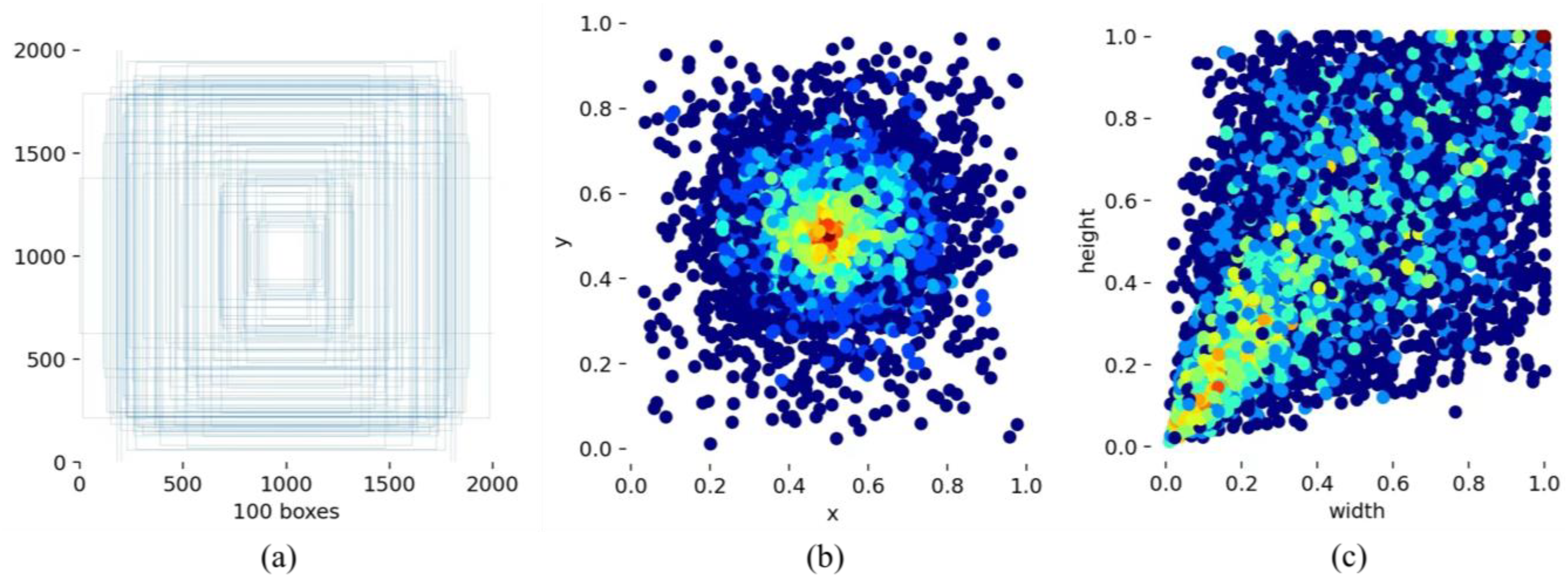
Figure 9 shows the number of object bounding boxes in each class of the COD10K dataset (COD10K dataset labels all subclasses as “foreground”), the distribution of the first 100 bounding boxes, the abscissa and ordinate of the center point of the camouflaged object, and the proportion of the bounding boxes of the camouflaged object in the image size.

We selected the commonly used average precision (AP) as the object detection evaluation index for testing, including AP_50–95 (indicating that the IOU was taken from 0.5 to 0.95 in steps of 0.05, and the APs under these IOU values were calculated separately and then averaged), AP₅₀ (AP value at an IOU of 0.5), AP₇₅ (AP value at an IOU of 0.75), AP_S (AP values for small targets with sizes less than 32²), AP_M (AP values for medium targets with sizes of 32² to 96²), and AP_L (AP values for targets with sizes greater than 96²).

4.3. Comparison Algorithms

To demonstrate the effectiveness of the CPNet proposed in this paper, we compared it with 17 classic and state-of-the-art methods. Each algorithm was trained and tested using two different backbone sizes. The proposed algorithm used the two different sizes of the Swin transformer backbone, which had a similar performance to the backbones used in the other algorithms; a comparison with the mainstream ResNet backbone can be seen in

Table 3. Comparison of the Swin transformer backbone with the ResNet backbone.

Backbone	Input Size	Params (M)	FLOPs (G)	Top-1 Acc (%)
ResNet50	224 × 224	23.28	4.12	76.1
Swin-T	224 × 224	27.50	4.36	81.3
ResNet101	224 × 224	42.28	7.85	77.4
Swin-S	224 × 224	48.79	8.52	83.0

. To fairly compare the detection performance of the algorithms, all algorithms used the experimental configuration platform described in Section 3.1, and the experimental parameters followed the default settings.

4.4. Analysis of the Comparative Experimental Results

In this paper, we first compared the CPNet with 17 algorithms quantitatively and qualitatively in a cross-sectional manner; later, to confirm the effectiveness of each module, ablation experiments were carried out.

4.4.1. Cross-Sectional Comparison Results

Quantitative comparison: The experimental results of the cross-sectional comparison between the CPNet proposed in this paper and 17 other algorithms on the COD10K camouflaged object dataset are shown in

Table 4. The experimental results obtained in cross-sectional comparison conducted on the COD10K dataset (the top three performances are highlighted in red, blue, and green, bold denotes our algorithm).

Methods	Pub. Year	Backbone	AP50–95	AP50	AP75	APS	APM	APL
Mask RCNN [16]	ICCV ‘2017	R50-FPN	39.73	71.43	39.97	6.20	24.78	44.10
		R101-FPN	43.04	73.94	43.98	7.34	25.95	47.86
Cascade RCNN [43]	TPAMI ‘2019	R50-FPN	42.91	70.78	44.61	8.87	24.63	47.94
		R101-FPN	46.32	73.56	48.44	8.40	27.99	51.48
YOLACT [46]	ICCV ‘2019	R50-FPN	33.95	67.43	30.71	7.69	17.80	38.32
		R101-FPN	36.54	69.89	34.68	6.11	19.65	41.09
Instaboost [47]	ICCV ‘2019	R50-FPN	42.99	72.02	44.52	4.46	24.81	48.12
		R101-FPN	46.97	74.18	50.02	7.28	28.25	52.36
HTC [48]	CVPR ‘2019	R50-FPN	44.22	73.30	44.85	11.42	28.23	48.86
		R101-FPN	47.28	74.98	49.16	10.62	29.18	52.37
BlendMask [49]	CVPR ‘2020	R50-FPN	41.51	69.99	42.06	4.74	25.54	46.17
		R101-FPN	43.63	68.63	45.50	7.68	25.24	48.90
ATSS [50]	CVPR ‘2020	R50-FPN	41.21	70.26	41.53	5.86	28.39	45.00
		R101-FPN	45.03	73.65	45.36	11.92	30.44	49.17
CondInst [51]	ECCV ‘2020	R50-FPN	40.38	67.72	40.84	6.63	24.56	45.03
		R101-FPN	42.86	69.45	44.61	5.88	24.74	47.95
BoxInst [52]	CVPR ‘2021	R50-FPN	37.30	65.98	36.86	9.83	21.03	41.86
		R101-FPN	40.66	68.66	40.15	7.24	25.05	45.30
SparseRCNN [53]	CVPR ‘2021	R50-FPN	41.82	72.98	40.72	13.14	32.11	45.14
		R101-FPN	46.53	74.95	47.96	12.46	34.30	50.47
VFNet [54]	CVPR ‘2021	R50-FPN	43.30	71.12	44.10	13.53	28.17	47.66
		R101-FPN	46.60	73.90	48.02	7.97	31.25	51.17
Tood [55]	ICCV ‘2021	R50-FPN	43.84	71.52	44.26	13.41	27.98	48.19
		R101-FPN	47.90	73.90	49.04	12.02	32.08	52.41
SCNet [56]	AAAI ‘2021	R50-FPN	44.30	74.39	44.67	11.78	28.63	48.70
		R101-FPN	47.10	75.55	48.24	13.80	29.01	52.02
Swin-RCNN [37]	ICCV ‘2021	Swin-T	45.11	77.08	46.85	11.13	28.25	49.63
		Swin-S	50.25	79.85	54.63	11.39	31.96	55.31
Centernet++ [57]	Arxiv ‘2022	R50-FPN	38.24	68.59	37.31	6.01	22.54	42.80
		R101-FPN	42.36	72.31	42.28	11.05	24.76	47.38
MaskTrans [21]	CVPR ‘2022	R50-FPN	40.35	68.29	42.08	5.87	23.10	45.06
		R101-FPN	46.32	70.03	48.82	3.56	27.78	51.49
MPVIT-RCNN [13]	CVPR ‘2022	MPVIT-T	50.87	79.81	54.02	13.43	33.70	55.83
		MPVIT-S	57.51	82.37	63.33	17.27	38.15	62.90
CPNet	Ours	Swin-T	52.26	86.25	57.84	15.01	45.65	55.17
		Swin-S	59.77	91.41	73.04	19.14	49.56	63.71

. The results obtained by each algorithm using the same backbone size were compared.

As can be seen from the table, the CPNet proposed in this paper had five metrics that were superior to those of the other algorithms when using a small backbone, and its AP_50–95 reached 52.26%, which was higher than MPVIT by 1.39%; its AP₅₀ was 6.44% higher, and AP₇₅ was 3.82% higher. The data showed that the AP value of the CPNet was still better when the IOU threshold was set higher. We can conclude that the CPNet had more advanced confidence compared to other approaches. When using a large backbone, the CPNet exerted its advantage of accurate camouflaged object detection, and all six indices were better than for the other algorithms, among which the AP₅₀ and AP₇₅ exceeded those of the MPVIT by approximately 10%. Again, this reflects the accuracy of the CPNet. By observing the last three columns in Table 4, CPNet had significant advantages with respect to the detection of small- and medium-sized targets, where all of the metrics were greatly improved.

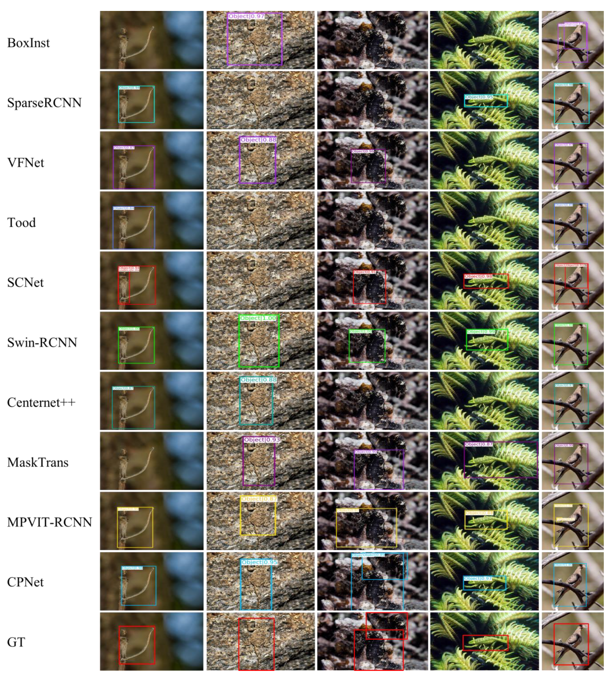
Qualitative comparison: From the quantitative analysis, it is clear that the metrics of the algorithms after 2021 gradually occupied the top three spots, so we selected the models after 2021 for visual comparison. Figure 10 shows the visualization results obtained by cross-sectional comparison experiments when using a large backbone. It can be seen that the CPNet proposed in this paper was more robust than the other methods. The FPM in the TCPM could extract the relationship information between features so that the algorithm better identified the interesting parts of the object that were difficult to identify, such as tentacles and tails (e.g., columns 1–2). The SPM in the TCPM could obtain the spatial information of the camouflaged object to improve the accuracy of the object bounding box and accurately detect multiple targets (e.g., columns 3–4). The KPM could extract the location information of the key points to locate targets precisely; thus, it reduced the false alarm and prevented bounding box selection from being repeated (e.g., column 5).

4.4.2. Ablation Experiments

To verify the effectiveness of the main CPNet modules and the three modules in the TCPM, we designed ablation experiments where the baseline network was the cascade RCNN algorithm.

Quantitative analysis:

Table 5. Longitudinal comparison results obtained in ablation experiments conducted on the COD10K dataset (the top three performances are highlighted in red, blue, and green).

Baseline	Swin	CAP	FPM	SPM	KPM	Backbone	AP50–95	AP50	AP75	APS	APM	APL
√						R50-FPN	42.91	70.78	44.61	8.87	24.63	47.94
						R101-FPN	46.32	73.56	48.44	8.40	27.99	51.48
√	√					Tiny	43.43	75.88	44.46	10.79	27.49	47.78
						Small	48.63	78.76	52.34	9.67	31.35	53.47
√	√	√				Tiny	47.24	80.20	50.20	2.38	33.86	52.57
						Small	50.73	84.13	57.30	5.50	40.76	54.39
√	√	√	√			Tiny	48.97	83.48	53.41	3.37	34.79	54.38
						Small	53.19	87.64	60.47	9.70	46.78	57.37
√	√	√	√	√		Tiny	50.07	85.45	54.54	4.36	39.39	54.17
						Small	56.81	89.95	67.23	12.12	48.62	60.69
√	√	√	√	√	√	Tiny	52.26	86.25	57.84	15.01	45.65	55.17
						Small	59.77	91.41	73.04	19.14	49.56	63.71

comprehensively shows the longitudinal comparison results of the ablation experiments conducted with the CPNet. It can be found that, compared to the baseline network, when using the Swin transformer backbone network and the cascaded aggregation network, the model outperformed or was on par with state-of-the-art models. For the TCPM, the three submodules were tested separately to verify the effectiveness of each submodule. The metrics were also significantly improved by adding the FPM to the network, but the effect of this module was mainly reflected in the feature maps (see the qualitative analysis). After adding the SPM, the comprehensive performance of the network already exceeded that of the MPVIT. The AP₇₅ improved by 6.76% when using a large backbone, which meant that the confidence in the detection results increased. Finally, after adding the KPM, the metrics were optimized, and the AP value was further improved because the KPM eliminated some of the false alarms.

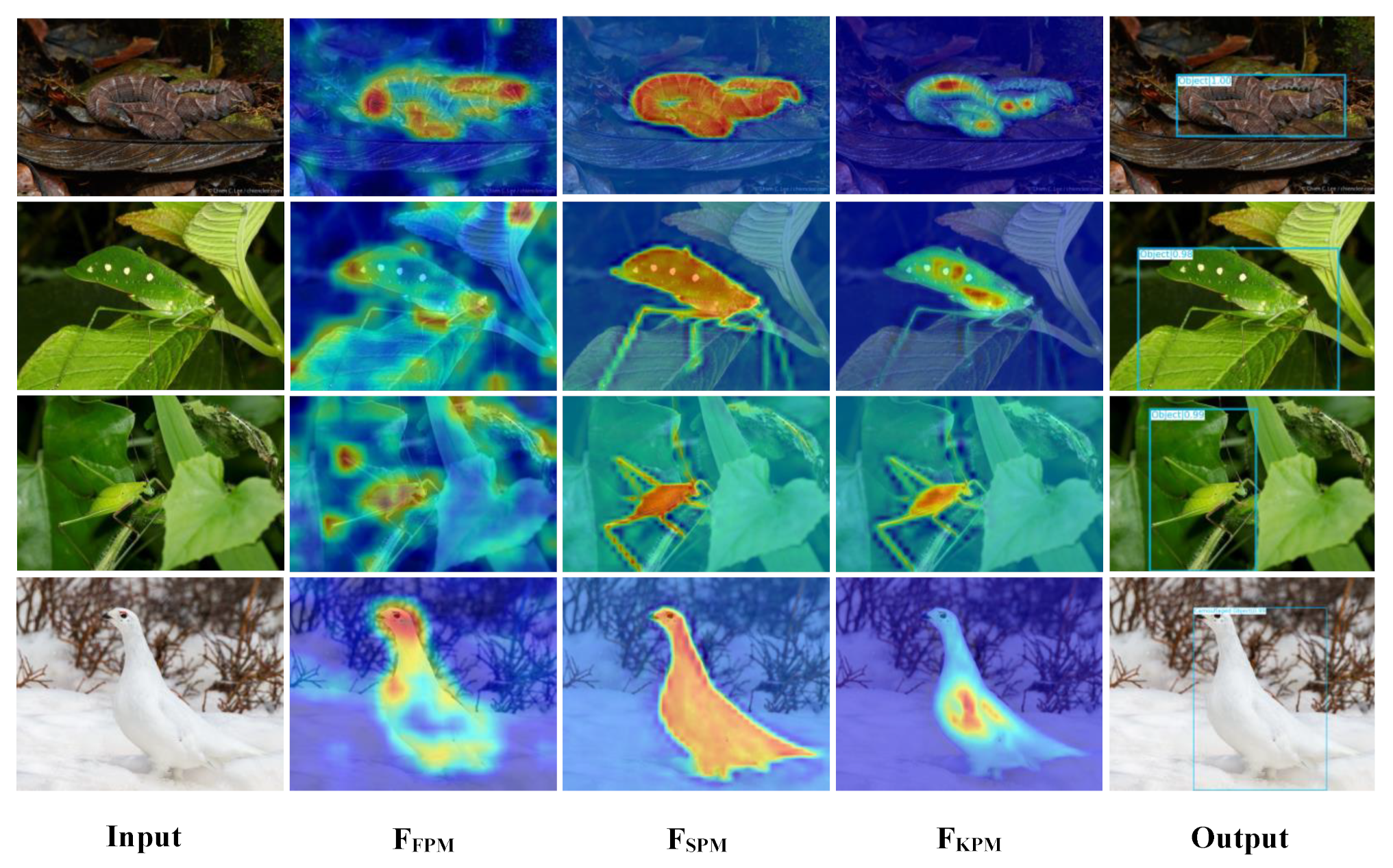
Qualitative analysis: This subsection focuses on the visual analysis of the effects of the three submodules of the TCPM. The feature maps resulting from adding the three sub-modules individually are visualized and fused with the original image, and the results are shown in Figure 11. F_FPM denotes the feature map of the FPM output, F_SPM denotes the feature map of the SPM output, and F_KPM denotes the feature map of the KPM output. After adding the FPM alone, the network could extract the relationship information between features, which enhanced the ability of the network to distinguish the key difference regions between the object and the background, such as the insect’s slender foot and tentacles in Figure 9. By adding the SPM alone, the network could learn the spatial information of the object, and all the regions where the object existed could be assigned higher weights. The CPNet extracted the key point location information and key region information of the object with the KPM module, as is shown in the figure. The weights gradually decreased from the center to the edge, thus reducing false alarms and improving the confidence of object detection.

4.5. Extended Experiments for Generalized Camouflaged Object Detection

As was mentioned in the introduction, the study of generalized COD, which refers to the detection of any object with low detectability in an image, is of great significance. Therefore, to prove that the CPNet proposed in this paper remained effective when extended to generalized COD, a series of extended experiments were conducted in this paper. Figure 12 shows the visualization results obtained when applying CPNet to the detection of small infrared targets; the dataset used was the FLIR thermal dataset [58]. Figure 13 shows the visualization results obtained when the network was applied to detection in extreme weather road conditions, and the dataset used was the foggy driving dataset [59]. Since generalized COD was not the focus of our study, in

Table 6. Experimental results on FLIR thermal dataset (the top three performances are highlighted in red, blue, and green, bold denotes our algorithm.).

Methods	Pub. Year	Backbone	AP50–95	AP50	AP75	APS	APM	APL
Centernet++ [57]	Arxiv ‘2022	R50-FPN	65.25	85.77	57.90	57.03	71.25	75.87
		R101-FPN	67.67	85.67	62.85	62.06	77.02	81.76
MaskTrans [21]	CVPR ‘2022	R50-FPN	69.58	88.92	61.98	58.47	73.07	75.06
		R101-FPN	72.62	85.83	65.59	59.69	77.64	79.98
MPVIT-RCNN [13]	CVPR ‘2022	MPVIT-T	77.93	92.64	73.28	71.88	85.96	89.88
		MPVIT-S	77.58	94.85	76.69	74.51	84.52	90.17
CPNet	Ours	Swin-T	74.67	91.70	75.44	75.03	85.26	90.24
		Swin-S	76.84	94.97	76.48	77.91	87.11	93.31

and

Table 7. Experimental results on foggy driving dataset (the top three performances are highlighted in red, blue, and green, bold denotes our algorithm.).

Methods	Pub. Year	Backbone	AP50–95	AP50	AP75	APS	APM	APL
Centernet++ [57]	Arxiv ‘2022	R50-FPN	42.24	74.10	40.41	23.53	53.04	56.72
		R101-FPN	43.34	75.43	37.92	22.65	54.57	64.90
MaskTrans [21]	CVPR ‘2022	R50-FPN	44.56	73.83	41.47	16.40	48.26	51.39
		R101-FPN	45.10	73.98	42.56	17.72	52.80	58.46
MPVIT-RCNN [13]	CVPR ‘2022	MPVIT-T	51.57	80.83	52.57	28.67	60.72	69.57
		MPVIT-S	55.48	83.32	55.38	27.90	64.53	72.93
CPNet	Ours	Swin-T	50.69	78.56	53.49	25.10	56.77	63.76
		Swin-S	53.44	81.47	57.28	29.47	59.94	67.57

, we only selected the latest published algorithms for comparison. Since the compared algorithms are excellent generalized detection algorithms, CPNet could not reach optimality in both tasks but still maintained a high detection capability. This is because, in these applications, similar to that in typical COD, the object to be detected had similar features to the background, or its boundaries were indistinguishable, so the object was difficult to identify. Moreover, it is worth noting that CPNet still has advantages in small object detection. The results showed that the CPNet can be extended to similar applications for generalized COD. The performance can be improved if the structure is improved for different tasks.

5. Conclusions

In this paper, we proposed a ternary cascade perception-based detection method and constructed a CPNet to solve the problems of missing detections and low detection confidence for the COD applications. The TCPM focuses on extracting the relationship information between features, the spatial information of the camouflaged object, and the location information of key points, and it fuses the representation in the deep networks more efficiently. For the loss function, the focal loss function was used to obtain the object class loss value, and the CIOU function was used to obtain the object bounding box loss value, as this joint training method is more robust. A cross-sectional comparison conducted on the challenging COD10K dataset demonstrated the comprehensive performance advantage of the CPNet in COD; CPNet outperformed or was on par with state-of-the-art models, and its AP₅₀ and AP₇₅ exceeded the MPVIT by 10%. The ablation experiments demonstrated the effectiveness of each proposed module. Finally, extended experiments were conducted to demonstrate the effectiveness of the CPNet when applied to generalized COD. We offer the community an initial model of generalized COD. In future work, we plan to introduce contrast learning into COD so that the network can learn parameters by comparing the feature differences between camouflaged and generic objects. In addition, the introduction of edge information to refine the detection effect can also be explored. Subsequently, we will also advance our research on generalized COD to motivate the translation of research results into practical applications.

References

1. Cuthill, I.C.; Stevens, M.; Sheppard, J.B.; Maddocks, T.; Párraga, C.A.; Troscianko, T. Disruptive coloration and background pattern matching. Nature 2005, 434, 72–74. [Google Scholar] [CrossRef]
2. Stuart-Fox, D.; Moussalli, A.; Whiting, M.J. Predator-specific camouflage in chameleons. Biol Lett. 2008, 4, 326–329. [Google Scholar] [CrossRef] [Green Version]
3. Li, C.; Sohn, K.; Yoon, J.; Pfister, T. CutPaste: Self-Supervised Learning for Anomaly Detection and Localization. In Proceedings of the 2021 IEEE/CVF Conference on Computer Vision and Pattern Recognition (CVPR), Nashville, TN, USA, 20–25 June 2021; pp. 9659–9669. [Google Scholar] [CrossRef]
4. He, Y.; Ding, Y.; Roth, H.R.; Zhao, C.; Xu, D. DiNTS: Differentiable Neural Network Topology Search for 3D Medical Image Segmentation. In Proceedings of the 2021 IEEE/CVF Conference on Computer Vision and Pattern Recognition (CVPR), Nashville, TN, USA, 20–25 June 2021; pp. 5837–5846. [Google Scholar] [CrossRef]
5. Smith, M.Q.R.P.; Ruxton, G.D. Camouflage in predators. Biol. Rev. Camb. Philos. Soc. 2020, 95, 1325–1340. [Google Scholar] [CrossRef]
6. Jiang, X.; Cai, W.; Yang, Z.; Xu, P.; Jiang, B. IARet: A lightweight multiscale infrared aerocraft recognition algorithm. Arab. J. Sci. Eng. 2022, 47, 2289–2303. [Google Scholar] [CrossRef]
7. Ding, Y.; Zhao, X.; Zhang, Z.; Cai, W.; Yang, N.; Zhan, Y. Semi-supervised locality preserving dense graph neural network with ARMA filters and context-aware learning for hyperspectral image classification. IEEE Trans Geosci. Remote Sens. 2022, 60, 1–12. [Google Scholar] [CrossRef]
8. Li, X.M.; Huang, Q.C. Target detection for infrared polarization image in the background of desert. In Proceedings of the 2017 IEEE 9th International Conference on Communication Software and Networks (ICCSN), Guangzhou, China, 6–8 May 2017; pp. 1147–1151. [Google Scholar] [CrossRef]
9. Suryanto, N.; Kim, Y.; Kang, H.; Larasati, H.; Yun, Y.; Le, T.; Yang, H.; Oh, S.; Kim, H. DTA: Physical Camouflage Attacks using Differentiable Transformation Network. arXiv 2022, arXiv:2203.09831. [Google Scholar] [CrossRef]
10. Zhang, Y.; Fan, Y.; Xu, M.; Li, W.; Zhang, G.; Liu, L.; Yu, D. An Improved Low Rank and Sparse Matrix Decomposition-Based Anomaly Target Detection Algorithm for Hyperspectral Imagery. IEEE J. Sel. Top. Appl. Earth Obs. Remote Sens. 2020, 13, 2663–2672. [Google Scholar] [CrossRef]
11. Chandesa, T.; Pridmore, T.P.; Bargiela, A. Detecting occlusion and camouflage during visual tracking. In Proceedings of the 2009 IEEE International Conference on Signal and Image Processing Applications, Kuala Lumpur, Malaysia, 18–19 November 2009; pp. 468–473. [Google Scholar] [CrossRef]
12. Mondal, A. Camouflaged Object Detection and Tracking: A Survey. Int. J. Image Graph. 2020, 20, 2050028:1–2050028:13. [Google Scholar] [CrossRef]
13. Lee, Y.; Kim, J.; Willette, J.; Hwang, S.J. MPViT: Multi-Path Vision Transformer for Dense Prediction. In Proceedings of the 2022 IEEE/CVF Conference on Computer Vision and Pattern Recognition (CVPR), New Orleans, LA, USA, 19–20 June 2022. [Google Scholar]
14. Zou, Z.; Shi, Z.; Guo, Y.; Ye, J. Object Detection in 20 Years: A Survey. arXiv 2019, arXiv:1905.05055. [Google Scholar] [CrossRef]
15. Wang, X.; Shrivastava, A.; Gupta, A.K. A-Fast-RCNN: Hard Positive Generation via Adversary for Object Detection. In Proceedings of the 2017 IEEE Conference on Computer Vision and Pattern Recognition (CVPR), Honolulu, HI, USA, 21–26 July 2017; pp. 3039–3048. [Google Scholar] [CrossRef] [Green Version]
16. He, K.; Gkioxari, G.; Dollar, P.; Girshick, R. Mask R-CNN. IEEE Trans Pattern Anal Mach Intell. 2020, 42, 386–397. [Google Scholar] [CrossRef]
17. Qiao, S.; Chen, L.; Yuille, A.L. DetectoRS: Detecting Objects with Recursive Feature Pyramid and Switchable Atrous Convolution. In Proceedings of the 2021 IEEE/CVF Conference on Computer Vision and Pattern Recognition (CVPR), Nashville, TN, USA, 20–25 June 2021; pp. 10208–10219. [Google Scholar] [CrossRef]
18. Redmon, J.; Divvala, S.K.; Girshick, R.B.; Farhadi, A. You Only Look Once: Unified.; Real-Time Object Detection. In Proceedings of the 2016 IEEE Conference on Computer Vision and Pattern Recognition (CVPR), Las Vegas, NV, USA, 27–30 June 2016; pp. 779–788. [Google Scholar] [CrossRef] [Green Version]
19. Duan, K.; Bai, S.; Xie, L.; Qi, H.; Huang, Q.; Tian, Q. CenterNet: Keypoint Triplets for Object Detection. In Proceedings of the 2019 IEEE/CVF International Conference on Computer Vision (ICCV), Seoul, Republic of Korea, 27–28 October 2019; pp. 6568–6577. [Google Scholar] [CrossRef] [Green Version]
20. Tan, M.; Pang, R.; Le, Q.V. EfficientDet: Scalable and Efficient Object Detection. In Proceedings of the 2020 IEEE/CVF Conference on Computer Vision and Pattern Recognition (CVPR), Seattle, WA, USA, 13–19 June 2020; pp. 10778–10787. [Google Scholar] [CrossRef]
21. Ke, L.; Danelljan, M.; Li, X.; Tai, Y.W.; Tang, C.K.; Yu, F. Mask Transfiner for High-Quality Instance Segmentation. In Proceedings of the 2022 IEEE/CVF Conference on Computer Vision and Pattern Recognition (CVPR), New Orleans, LA, USA, 19–20 June 2022. [Google Scholar]
22. Zhang, J.M.; Ye, Z.; Jin, X.K.; Wang, J.; Zhang, J. Real-time traffic sign detection based on multiscale attention and spatial information aggregator. J. Real-Time Image Processing. 2022, 19, 1155–1167. [Google Scholar] [CrossRef]
23. Zhang, Z.; Ding, Y.; Zhao, X.; Li, S.; Yang, N.; Cai, Y.; Zhan, Y. Multireceptive field: An adaptive path aggregation graph neural framework for hyperspectral image classification. Expert Syst. Appl. 2023, 217, 119508. [Google Scholar] [CrossRef]
24. Zhang, J.M.; Zheng, Z.F.; Xie, X.D.; Gui, Y.; Kim, G.J. ReYOLO: A traffic sign detector based on network reparameterization and features adaptive weighting. J. Ambient. Intell. Smart Environ. 2022, 14, 317–334. [Google Scholar] [CrossRef]
25. Huang, Z.; Li, W.; Xia, X.; Tao, R. A General Gaussian Heatmap Label Assignment for Arbitrary-Oriented Object Detection. IEEE Trans. Image Process. 2021, 31, 1895–1910. [Google Scholar] [CrossRef] [PubMed]
26. Huang, Z.; Li, W.; Xia, X.; Wang, H.; Tao, R. Task-wise Sampling Convolutions for Arbitrary-Oriented Object Detection in Aerial Images. arXiv 2022, arXiv:2209.02200. [Google Scholar]
27. Zhang, J.M.; Zou, X.; Kuang, L.D.; Wang, J.; Sherratt, R.S.; Yu, X.F. CCTSDB 2021: A more comprehensive traffic sign detection benchmark. Hum.-Cent. Comput. Inf. Sci. 2022, 12, 23. [Google Scholar] [CrossRef]
28. Liu, N.; Li, W.; Wang, Y.J.; Tao, R.; Du, Q.; Chanussot, J. A survey on hyperspectral image restoration: From the view of low-rank tensor approximation. Sci. China Inf. Sci. 2023, 66, 140302. [Google Scholar] [CrossRef]
29. Li, S.T.; Dian, R.W.; Liu, H.B. Learning the external and internal priors for multispectral and hyperspectral image fusion. Sci. China Inf. Sci. 2023, 66, 140303. [Google Scholar] [CrossRef]
30. Fan, D.P.; Ji, G.P.; Sun, G.; Cheng, M.M.; Shen, J.; Shao, L. Camouflaged object detection. In Proceedings of the 2020 IEEE/CVF conference on computer vision and pattern recognition (CVPR), Seattle, WA, USA, 13–19 June 2020; pp. 2774–2784. [Google Scholar] [CrossRef]
31. Mei, H.; Ji, G.P.; Wei, Z.; Yang, X.; Wei, X.; Fan, D.P. Camouflaged object segmentation with distraction mining. In Proceedings of the 2021 IEEE/CVF conference on computer vision and pattern recognition (CVPR), Nashville, TN, USA, 20–25 June 2021; pp. 8768–8777. [Google Scholar] [CrossRef]
32. Jiang, X.H.; Cai, W.; Jiang, B.; Yang, Z.Y.; Wang, X. MAGNet: A Camouflage Object Detection Network Simulating The Observation Effect of Magnifier. Entropy 2022, 24, 1804. [Google Scholar] [CrossRef]
33. Lv, Y.; Zhang, J.; Dai, Y.; Li, A.; Liu, B.; Barnes, N. Simultaneously localize; segment and rank the camouflaged objects. In Proceedings of the 2021 IEEE/CVF Conference on Computer Vision and Pattern Recognition (CVPR), Nashville, TN, USA, 20–25 June 2021; pp. 11586–11596. [Google Scholar] [CrossRef]
34. Pang, Y.; Zhao, X.; Xiang, T.; Zhang, L.; Lu, H. Zoom In and Out: A Mixed-scale Triplet Network for Camouflaged Object Detection. In Proceedings of the 2022 IEEE/CVF Conference on Computer Vision and Pattern Recognition (CVPR), New Orleans, LA, USA, 19–20 June 2022; pp. 2150–2160. [Google Scholar] [CrossRef]
35. Chu, X.; Zheng, A.; Zhang, X.; Sun, J. Detection in Crowded Scenes: One Proposal. Multiple Predictions. In Proceedings of the 2020 IEEE/CVF Conference on Computer Vision and Pattern Recognition (CVPR), Seattle, WA, USA, 13–19 June 2020; pp. 12211–12220. [Google Scholar] [CrossRef]
36. Meng, F.; Li, Y.; Shao, F.; Yuan, G.; Dai, J.Y. Visual-simulation region proposal and generative adversarial network based ground military target recognition. Def. Technol. 2021. [Google Scholar] [CrossRef]
37. Liu, Z.; Lin, Y.; Cao, Y.; Hu, H.; Wei, Y.; Zhang, Z.; Lin, S.; Guo, B. Swin Transformer: Hierarchical Vision Transformer using Shifted Windows. In Proceedings of the 2021 IEEE/CVF International Conference on Computer Vision (ICCV), Nashville, TN, USA, 20–25 June 2021; pp. 9992–10002. [Google Scholar] [CrossRef]
38. Deng, J.; Dong, W.; Socher, R.; Li, L.; Li, K.; Fei-Fei, L. ImageNet: A large-scale hierarchical image database. In Proceedings of the 2009 IEEE Conference on Computer Vision and Pattern Recognition, Miami, FL, USA, 20–25 June 2009; pp. 248–255. [Google Scholar] [CrossRef] [Green Version]
39. Lin, T.; Dollár, P.; Girshick, R.B.; He, K.; Hariharan, B.; Belongie, S.J. Feature Pyramid Networks for Object Detection. In Proceedings of the 2017 IEEE Conference on Computer Vision and Pattern Recognition (CVPR), Nashville, TN, USA, 20–25 June 2021; pp. 936–944. [Google Scholar] [CrossRef] [Green Version]
40. Chen, L.; Papandreou, G.; Kokkinos, I.; Murphy, K.P.; Yuille, A.L. DeepLab: Semantic Image Segmentation with Deep Convolutional Nets.; Atrous Convolution.; and Fully Connected CRFs. IEEE Trans. Pattern Anal. Mach. Intell. 2018, 40, 834–848. [Google Scholar] [CrossRef] [PubMed] [Green Version]
41. Kipf, T.; Welling, M. Semi-Supervised Classification with Graph Convolutional Networks. arXiv 2017, arXiv:1609.02907. [Google Scholar]
42. Wu, Y.; He, K. Group Normalization. Int. J. Comput. Vis. 2020, 128, 742–755. [Google Scholar] [CrossRef]
43. Cai, Z.; Vasconcelos, N. Cascade R-CNN: Delving Into High Quality Object Detection. In Proceedings of the 2018 IEEE/CVF Conference on Computer Vision and Pattern Recognition, Salt Lake City, UT, USA, 18–23 June 2018; pp. 6154–6162. [Google Scholar] [CrossRef] [Green Version]
44. Lin, T.; Goyal, P.; Girshick, R.B.; He, K.; Dollár, P. Focal Loss for Dense Object Detection. IEEE Trans. Pattern Anal. Mach. Intell. 2020, 42, 318–327. [Google Scholar] [CrossRef] [PubMed] [Green Version]
45. Zheng, Z.; Wang, P.; Liu, W.; Li, J.; Ye, R.; Ren, D. Distance-IoU Loss: Faster and Better Learning for Bounding Box Regression. AAAI 2020, 34, 12993–13000. [Google Scholar] [CrossRef]
46. Bolya, D.; Zhou, C.; Xiao, F.; Lee, Y.J. YOLACT: Real-Time Instance Segmentation. In Proceedings of the 2019 IEEE/CVF International Conference on Computer Vision (ICCV), Seoul, Republic of Korea, 27–28 October 2019; pp. 9156–9165. [Google Scholar] [CrossRef] [Green Version]
47. Fang, H.; Sun, J.; Wang, R.; Gou, M.; Li, Y.; Lu, C. InstaBoost: Boosting Instance Segmentation via Probability Map Guided Copy-Pasting. In Proceedings of the 2019 IEEE/CVF International Conference on Computer Vision (ICCV), Seoul, Republic of Korea, 27–28 October 2019; pp. 682–691. [Google Scholar] [CrossRef] [Green Version]
48. Chen, K.; Pang, J.; Wang, J.; Xiong, Y.; Li, X.; Sun, S.; Feng, W.; Liu, Z.; Shi, J.; Ouyang, W.; et al. Hybrid Task Cascade for Instance Segmentation. In Proceedings of the 2019 IEEE/CVF Conference on Computer Vision and Pattern Recognition (CVPR), Seoul, Republic of Korea, 27–28 October 2019; pp. 4969–4978. [Google Scholar] [CrossRef] [Green Version]
49. Chen, H.; Sun, K.; Tian, Z.; Shen, C.; Huang, Y.; Yan, Y. BlendMask: Top-Down Meets Bottom-Up for Instance Segmentation. In Proceedings of the 2020 IEEE/CVF Conference on Computer Vision and Pattern Recognition (CVPR), Seattle, WA, USA, 13–19 June 2020; pp. 8570–8578. [Google Scholar] [CrossRef]
50. Zhang, S.; Chi, C.; Yao, Y.; Lei, Z.; Li, S. Bridging the Gap Between Anchor-Based and Anchor-Free Detection via Adaptive Training Sample Selection. In Proceedings of the 2020 IEEE/CVF Conference on Computer Vision and Pattern Recognition (CVPR), Seattle, WA, USA, 13–19 June 2020; pp. 9756–9765. [Google Scholar] [CrossRef]
51. Tian, Z.; Shen, C.; Chen, H. Conditional Convolutions for Instance Segmentation. ECCV 2020, 2020, 282–298. [Google Scholar] [CrossRef]
52. Tian, Z.; Shen, C.; Wang, X.; Chen, H. BoxInst: High-Performance Instance Segmentation with Box Annotations. In Proceedings of the 2021 IEEE/CVF Conference on Computer Vision and Pattern Recognition (CVPR), Nashville, TN, USA, 20–25 June 2021; pp. 5439–5448. [Google Scholar] [CrossRef]
53. Sun, P.; Zhang, R.; Jiang, Y.; Kong, T.; Xu, C.; Zhan, W.; Tomizuka, M.; Li, L.; Yuan, Z.; Wang, C.; et al. Sparse R-CNN: End-to-End Object Detection with Learnable Proposals. In Proceedings of the 2021 IEEE/CVF Conference on Computer Vision and Pattern Recognition (CVPR), Nashville, TN, USA, 20–25 June 2021; pp. 14449–14458. [Google Scholar] [CrossRef]
54. Zhang, H.; Wang, Y.; Dayoub, F.; Sunderhauf, N. VarifocalNet: An IoU-aware Dense Object Detector. In Proceedings of the 2021 IEEE/CVF Conference on Computer Vision and Pattern Recognition (CVPR), Nashville, TN, USA, 20–25 June 2021; pp. 8510–8519. [Google Scholar] [CrossRef]
55. Feng, C.; Zhong, Y.; Gao, Y.; Scott, M.R.; Huang, W. TOOD: Task-aligned One-stage Object Detection. In Proceedings of the 2021 IEEE/CVF International Conference on Computer Vision (ICCV), Virtual, 11–17 October 2021; pp. 3490–3499. [Google Scholar] [CrossRef]
56. Vu, T.; Kang, H.; Yoo, C.D. SCNet: Training Inference Sample Consistency for Instance Segmentation. AAAI 2021, 35, 2701–2709. [Google Scholar] [CrossRef]
57. Duan, K.; Bai, S.; Xie, L.; Qi, H.; Huang, Q.; Tian, Q. CenterNet++ for Object Detection. arXiv 2022, arXiv:2204.08394. [Google Scholar]
58. FLIR Systems, Inc. FLIR Thermal Dataseted. [DB/OL]. 2019. Available online: https://www.flir.cn/oem/adas/adas-dataset-form/ (accessed on 29 December 2022).
59. Sakaridis, C.; Dai, D.; Gool, L.V. Semantic Foggy Scene Understanding with Synthetic Data. Int. J. Comput. Vis. 2018, 126, 973–992. [Google Scholar] [CrossRef] [Green Version]
Figure 1. Examples of camouflaged object detection (COD).
Remotesensing 15 01188 g001
Figure 2. The difference between generic object and camouflaged object. (a) Generic object; (b) Camouflaged object.
Remotesensing 15 01188 g002
Figure 3. Cascade perception network (CPNet) structure.
Remotesensing 15 01188 g003
Figure 4. Comparison among feature fusion networks.
Remotesensing 15 01188 g004
Figure 5. Ternary cascade perception module (TCPM) structure.
Remotesensing 15 01188 g005
Figure 6. Graph convolution network (GCN) schematic diagram.
Remotesensing 15 01188 g006
Figure 7. Improved batch normalization schematic diagram. (a) BatchNorm; (b) Improved BatchNorm.
Remotesensing 15 01188 g007
Figure 8. Key point perception module (KPM) schematic diagram. (a) key point location information perception. (b) receptive field enhancement.
Remotesensing 15 01188 g008
Figure 9. Overview of COD10K dataset. (a) The distribution of the first 100 bounding boxes; (b) The abscissa and ordinate of the center point of the camouflaged object; (c) The proportion of the bounding boxes of the camouflaged object in the image size.
Remotesensing 15 01188 g009
Figure 10. The visualization results obtained by all algorithms in the cross-sectional comparison experiments. (GT represents ground truth).
Remotesensing 15 01188 g010
Figure 11. Visual comparison results of the ablation experiment.
Remotesensing 15 01188 g011
Figure 12. Visualization of the detection results obtained on the FLIR thermal dataset.
Remotesensing 15 01188 g012
Figure 13. Visualization of detection results on the foggy driving dataset.
Remotesensing 15 01188 g013