Article

Bi-Kernel Graph Neural Network with Adaptive Propagation Mechanism for Hyperspectral Image Classification

Xi’an Research Institute of High Technology, Xi’an 710025, China
*
Author to whom correspondence should be addressed.
Remote Sens. 2022, 14(24), 6224; https://doi.org/10.3390/rs14246224
Submission received: 24 October 2022 / Revised: 29 November 2022 / Accepted: 6 December 2022 / Published: 8 December 2022

Abstract

:
Graph neural networks (GNNs) have been widely applied for hyperspectral image (HSI) classification, due to their impressive representation ability. It is well-known that typical GNNs and their variants work under the assumption of homophily, while most existing GNN-based HSI classification methods neglect the heterophily that is widely present in the constructed graph structure. To deal with this problem, a homophily-guided Bi-Kernel Graph Neural Network (BKGNN) is developed for HSI classification. In the proposed BKGNN, we estimate the homophily between node pairs according to a learnable homophily degree matrix, which is then applied to change the propagation mechanism by adaptively selecting two different kernels to capture homophily and heterophily information. Meanwhile, the learning process of the homophily degree matrix and the bi-kernel feature propagation process are trained jointly to enhance each other in an end-to-end fashion. Extensive experiments on three public data sets demonstrate the effectiveness of the proposed method.

1. Introduction

Hyperspectral images captured by hyperspectral sensors can provide a wealth of spectral information to uniquely identify various land-covers according to their reflective spectra. Hence, they have been extensively employed in numerous remote sensing fields, including clustering [1], classification [2], unmixing [3], change detection [4], and target or anomaly detection [5,6,7]. Among these areas, hyperspectral image classification (HSIC) is a common task and a crucial procedure, referring to categorizing each image pixel into a certain meaningful class, according to the image contents [8].
To date, various approaches have been proposed for HSI classification. Early research primarily relied on traditional pattern recognition techniques, such as the k-nearest neighbor classifier [9], support vector machines (SVM) [10,11], and sparse representation [12]. However, these classifiers ignore the sensitivity to spectral fluctuation in raw HSI and solely take into account the original spectral information of pixels in the HSI. In this case, many works have focused on extracting additional discriminative spectral features or investigating spatial–spectral properties of HSI for classification. For example, principal component analysis (PCA) and linear discriminant analysis (LDA) have been applied to reduce redundancy and extract low-dimensional spectral information from HSIs [13,14]. Furthermore, spatial information is often exploited by morphological profiles (EMPs) [15], morphological attribute profiles (APs) [16], Gabor filters [17], and so on. Due to the enhanced spectral and spatial characteristics, the classification performance can be somewhat improved [18].
However, the aforementioned methods are all based on handcrafted characteristics, which heavily rely on professional experience and are quite empirical [19]. To mitigate the limitations of hand-crafted feature design, deep learning techniques have been extensively employed in the area of HSIC, through the use of various advanced deep networks. For instance, deep belief networks (DBNs) [20] and recurrent neural networks (RNNs) [21] have been adopted to extract deep features. To further exploit the original spatial structure of the HSI, convolutional neural networks (CNNs) with 2D and 3D convolutions have been extensively used for HSIC. For example, Hong et al. [22] have applied a 2-D CNN to capture spectral–spatial information from various modalities to improve the effectiveness of HSI classification. Hamida et al. [23] have designed a joint spectral and spatial information process through the use of a 3D CNN architecture. A spectral–spatial 3D–2D CNN classification model has been introduced [24], which demonstrated the excellent potential of hybrid networks mixing two- and three-dimensional convolution for the deep extraction of spectral–spatial features. Furthermore, deeper models with advanced networks have been proposed, including capsule networks [25], recursive autoencoders [26], and transformers [27].
Although current CNN-based methods have demonstrated significant effectiveness in the HSIC task, the limitations of the convolutional operation itself hinder further improvement of their performance. First, CNNs commonly possess a large number of training parameters and are prone to over-fitting due to a lack of training data as, unfortunately, there is a widespread problem with small training samples in the remote sensing field. Second, CNNs generally obfuscate the classification boundary as they use a kernel of fixed shape around the central pixel [28]. For these reasons, precise categorization of HSIs is still difficult. Finally, CNNs commonly apply patch-based neighborhoods of samples with fixed sizes as input; however, this approach cannot determine the homophily between pixels within and outside of the patch [29].
Considering the difficulties mentioned above, one possible solution is to design graph-based semi-supervised models that exploit the latent relationships between labeled and unlabeled data. Many GNN-based HSIC methods have recently been proposed for the extraction of features by considering the whole HSI as graph structure data. Normally, the success of GNN-based HSI classification algorithms relies on the propagation capability and the efficiency of the adjacency matrix. The propagation capability is usually achieved using a classical graph neural network model, such as GCN [30], GAT [31], EdgeConv [32], or GraphSage [33]. Typical works that apply these models in HSIC include [34,35,36,37,38]. Meanwhile, the adjacency matrix describes the similarity between two nearby pixels or superpixels. Early GNN-based approaches constructed pixel-level graphs by treating each pixel as a node in the graph [22,34], which can directly propagate information between nearby and distant regions; however, this will result in a vast amount of computation and limits its applicability, due to hundreds of thousands of pixels in an HSI. Fortunately, superpixel, which can effectively characterize the spatial semantic information of surface objects, provides a reasonable way to solve this problem [39,40,41]. In addition, as the number of labels is implicitly expanded in superpixels, the problem of small samples can be mitigated, to some extent [35]. Therefore, we focus on superpixel-based GNN models in our research.
Although GNNs have revealed remarkable advantages in the task of HSI classification, it has been neglected that GNN-based methods are widely believed to work well when dealing with homophily graphs, and fail to generalize to heterophily graphs when dissimilar nodes are connected [42,43]. Due to the diverse transformations in the graph construction of hyperspectral images, how can we ensure the high homophily of the graph data? As far as we know, previous GNN-based HSIC methods have not considered this problem. Noting that the homophily property can be quantitatively measured by the Homophily Ratio (HR) [44], we were inspired to determine different feature transformations through a learnable kernel, according to the homophily calculation among different local regions in a graph. However, in the HSI classification scenario, a high homophily level cannot easily determine better performance. We know that homophily is only related to the number of superpixels when the way of constructing the graph is determined. As shown on the left of Figure 1, we can see that the homophily level increases as the number of superpixels increases in both data sets, while the classification performance does not always increase with an increasing number of superpixels. As can be seen from the right of Figure 1, the overall accuracy (OA) suffers a slight decline with a large number of superpixels for both data sets. This is because most previous methods only use the same kernel to transform the features of neighbors; in this way, a large number of superpixels may lose the power to explore local spatial information of the HSI, even if the homophily level is improved. Therefore, we cannot infinitely improve the homophily level of the graph by increasing the number of superpixels. As a result, the heterophily information that exists in the constructed graph cannot be neglected.
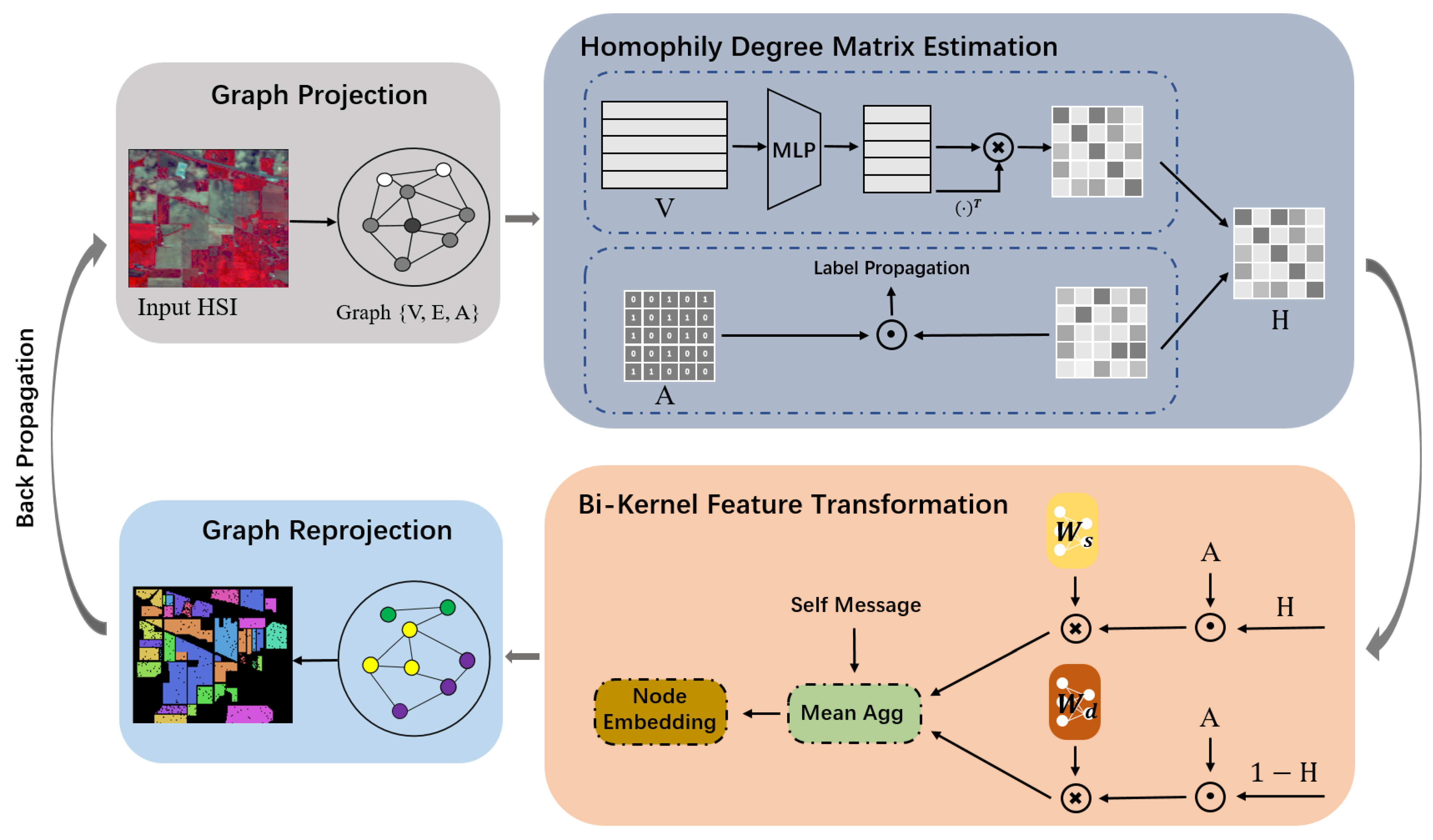
In this paper, we propose a bi-kernel graph neural network with adaptive propagation mechanism (BKGNN) for HSI classification. In particular, a homophily degree matrix learned from the attribute and topological information is applied to model the homophily and heterophily of the graph, and is further used to adaptively change the propagation process. To avoid smoothing distinguishable features, we use bi-kernels to propagate information on the graph, with one for homophily node pairs and the other for heterophily node pairs. To make the proposed approach more easy to understand, a schematic of BKGNN is displayed in Figure 2. Compared with traditional GNN-based HSI classification algorithms, the main contributions of this paper are as follows:
1.
We introduce a novel homophily degree matrix to estimate the homophily and heterophily that widely exist in the constructed graph for HSI. In the process of homophily degree matrix estimation, topological features and attribute features are learned by label propagation (LP) and Multilayer Perception (MLP) through extracting class-aware information. Thus, we can incorporate the homophily and heterophily information into the graph convolution framework.
2.
We propose a homophily-guided bi-kernel propagation mechanism, through which we can automatically change the feature propagation process by utilizing both homophily and heterophily information from the graph. To the best of our knowledge, this is the first time that a homophily-guided GNN technique has been applied to the HSI classification task.
3.
Extensive experiments on three real-world data sets, i.e., Indian Pines, Pavia University, and Kennedy Space Center, are conducted to validate the performance of the proposed BKGNN both qualitatively and quantitatively. The experimental results demonstrate a significant improvement over previous methods.

2. Methodology

In this section, we first provide some preliminaries of our method by reviewing some basic definitions and notation, including calculation of the homophily ratio, and an introduction to GNN and LP. Then the proposed BKGNN is illustrated in detail. The main notation adopted in our manuscript and relevant descriptions are provided in Table 1. All symbols in the article are explained in detail in the corresponding place.

2.1. Preliminaries

2.1.1. Graph Neural Network (GNN)

Graph neural networks, which operate on graph data, have demonstrated their effectiveness in various graph tasks. Let G = ( V , E ) represent the graph obtained from the original HSI data, where V = { v 1 , v 2 , , v n } is the set of vertices and E is the set of edges, representing the connectivity between vertices in V . Generally, a GNN follows a message-passing mechanism, which commonly consists of a message aggregation phase and an update phase. During the message passing phase [45], the representation z v of node v i is iteratively updated based on message m v , according to
m v l + 1 = w N ( v ) M ( z v l , z w l , e v w ) ,
z v l + 1 = U ( z v l , m v l + 1 ) ,
where M is a node feature aggregation function, which is a differential permutation-invariant operation; and U is the vertex message update function; N ( v ) denotes the nodes neighboring v in G ; and z v l and z v l + 1 are the representation vectors of node v at the l th and ( l + 1 ) th layers, respectively.
These two functions (i.e., M and U) can take a variety of forms [46]. Concretely, the aggregation function can be a mean aggregator, a max-pooling aggregator, an attention aggregator, or an LSTM aggregator. Meanwhile, the update function is usually achieved by a multi-layer perceptron or a gated network. For example, the GCN model [30] uses a message function M ( z v l , z w l ) = c v w z w l , where c v w = ( d e g ( v ) d e g ( w ) ) 1 / 2 A v w . The vertex update function is U ( z v l , m v l + 1 ) = R e L U ( W l m v l + 1 ) . The GNN-based HSIC approach is essentially a semi-supervised node classification task. Let Y { 0 , 1 } N × C denote the labels of nodes, where C is the number of classes, while only the first m nodes ( 0 < m n ) have labels Y L . The objective is to learn a predictive function to infer the missing labels Y U for the remaining n m nodes.

2.1.2. Homophily in Graphs

As we need to improve the graph convolution operation based on the homophily of the graph, we first need to determine how to measure the degree of homophily in graphs. We use the homophily ratio to measure the overall homophily level in a graph, which counts the fraction of edges connecting nodes that have the same labels. Formally, the homophily ratio is defined as:
h = 1 | E | ( v i , v j ) E 1 y i = y j ,
where | E | denotes the number of edges in the graph, and  1 is the indicator function. In accordance with the definition, we have h [ 0 , 1 ] . A graph with high homophily ratio is considered to be highly homophilous. Correspondingly, the node-level homophily is defined as
h i = 1 | N ( v i ) | v j N ( v i ) 1 y i = y j ,
where | N ( v i ) | is the size of the neighbor set N ( v i ) . Compared with the homophily ratio which is regarded as a global property in the whole graph, the node-level homophily focus on the local regions in a graph, and there may be different levels of homophily among different local regions in a homophily graph.
It is difficult to estimate the homophily level directly from node labels, as there are only a scarce number of nodes with labels in a semi-supervised task. We introduce a matrix H R n × n with its i j th element defined as the possibility that the corresponding two points (i.e., v i and v j ) belong to the same category. Note that H i j = 1 if v i and v j have the same label, and  H i j = 0 if v i and v j have no edge connection. The matrix H is called the homophily degree matrix in our algorithm, which will be discussed in detail in Section 2.4.

2.1.3. Label Propagation (LP) Algorithm

In the process of calculating the homophily degree matrix, we use LP to estimate the homophily degree between node pairs from the topological space. Let Y 0 represent the initial label matrix Y . The rows of Y 0 corresponding the labeled nodes are one-hot indicator vectors, and the unlabeled nodes are zero vectors. Label propagation is often applied to infer pseudo-labels for unlabeled nodes based on Y 0 . Assuming that neighboring nodes are more likely to have the same label, LP propagates labels along the edges iteratively. It is feasible to specify the formulation of the LP algorithm in iteration l as follows:
Y ( l ) = D 1 A Y ( l 1 ) ,
where A R N × N denotes the adjacency matrix, whose elements a i j denote the non-negative pairwise similarity between v i and v j ; D is the diagonal matrix of A , with entries d i i = j a i j ; and Y ( l ) is the pseudo-label matrix in iteration l. As the adjacency matrix A is a sparse matrix with non-zero elements on nearest neighbors, the true label information will propagate from each labeled example to its neighbors in each iteration.

2.2. Overall Framework

As shown in Figure 2, the proposed BKGNN consists of four main modules: graph projection, homophily degree matrix estimation, bi-kernel feature transformation, and graph re-projection. The first module maps the original pixel-level HSI data X R H × W × B to a superpixel-level graph structure G = ( V , E ) , where V denotes the group of obtained superpixels, which can be represented by an attribute matrix V R N × B , while E can be represented by a spatial adjacency matrix A R N × N . We apply a multi-layer perceptron (MLP) and the label propagation (LP) technique to extract the homophily information from the attribute space and topological space, respectively, and define the whole homophily degree matrix H R N × N based on these two types of information. After that, the bi-kernel feature transformation trains W s and W d to capture the similarity between nodes and the dissimilarity between nodes. The homophily degree matrix obtained from the former module is utilized to combine these two processes of message passing, producing the superpixel-level node embedding. Furthermore, self-messages are added into the procedure of computing the node embedding, in order to reduce over-smoothing. The enhanced superpixel features are then projected to pixel features by the last module, which is used to perform pixel-wise classification. In the proposed BKGNN, the cross-entropy loss function is utilized to minimize the differences between the predicted labels and the ground-truth of training samples. The details of these modules are described in the following.

2.3. Graph Projection and Re-Projection

To reduce the computational complexity while maintaining the local structure of the HSI, GNN-based HSI classification models frequently operate on superpixel-based nodes, rather than pixel-based nodes. Therefore, we establish the relationship between pixel-level HSI data and the superpixel-level graph structure. For this purpose, we pre-process the entire image into a number of spatially linked superpixels using the simple linear iterative clustering (SLIC) method. Considering each superpixel as a graph node, each superpixel’s average spectral signature serves as the node feature, and edge connections are established between neighboring nodes. Consequently, the superpixel-level graph structure G = ( V , E ) can be obtained.
Specifically, the graph projection assigns the original HSI data I to a set of nodes V and determines the corresponding feature matrix V through matrix multiplication, as follows:
V = Q ^ T Flatten ( X ) ,
where Q ^ is the normalized Q by column (i.e., Q ^ i , j = Q i , j / m Q m , j ), and Flatten ( · ) represents flattening the HSI data by the spatial dimension. The association matrix Q R H W × N is introduced by SLIC, which is defined as
Q i , j = 1 , i f x i S j , 0 , otherwise ,
where S i is the i th superpixel that consists of several homogeneous pixels.
As for the edge set E , two superpixels that share a common boundary are considered to have an edge connection. Thus, the adjacency matrix A related to E can be defined as
A i , j = 1 , i f if S i and S j are adjacent 0 , otherwise ,
where S i and S j denote the i th and j th superpixels, respectively.
We use graph re-projection to convert the generated features back to the original coordinate space for pixel-wise classification. The transformed node features V ˜ R N × C and the assignment matrix Q are used as inputs for the graph re-projection process, which outputs the appropriate 3D feature map. This operation is defined as
X ˜ = Reshape ( Q V ˜ ) ,
where Reshape(·) denotes restoring the spatial dimension of the flattened data.

2.4. Homophily Degree Matrix Calculation

Conventional GNN models have fundamental homophily assumptions and, as such, are not suited for heterophily graphs [42]. As shown in Figure 1, even if we can reduce the degree of heterogeneity of the graph to some extent by setting an appropriate superpixel size, the heterogeneity of the graph cannot be ignored. To solve this problem, we introduce a homophily degree matrix H R N × N , with its ( i , j ) th element defining the extent to which the i th and j th nodes belong to the same class. However, it is difficult to calculate the homophily degree directly from node labels, as only a small number of labels are known in the context of the semi-supervised task. In order to fill this gap, we estimate the soft labels for unlabeled nodes from the attribute space and topological space.
To utilize the attribute space of the graph, we apply a graph-agnostic multi-layer perceptron (MLP) to generate soft labels from the original node attributes. The l th layer of the MLP is defined as:
Z ( l ) = σ ( Z ( l 1 ) W ( l ) ) ,
where W ( l ) is the learnable weight matrix, and  σ ( · ) is an activation function. Denoting by Z the output of MLP for several iterations, the soft assignment matrix B R N × C can be obtained, using a softmax operation, as follows:
B = softmax ( Z ) .
Let Θ m denote all the parameters of the MLP. Then, the optimal Θ m * can be obtained by minimizing the loss function:
Θ m * = argmin Θ L m l p = argmin Θ m v i T V J ( b i , y i ) ,
where b i is the predicted soft label of node v i , y i is the ground-truth label of v i , T V denotes the nodes in the training set, and  J ( · ) is the cross-entropy.
In terms of the topological space, we further apply the label propagation (LP) technique to estimate the soft labels. We generalize classic LP with a learnable weight matrix T R N × N . Similar to Equation (5), the resulting generalized LP in the l th iteration is defined as:
Y ( l ) = D ^ 1 ( A T ) Y ( l 1 ) ,
where D ^ is the diagonal matrix for matrix A T . Similar to MLP optimization, the optimal weight matrix T is learned by
T * = argmin T L l p = argmin T v i T V J ( y i l p , y i ) .
Finally, the homophily degree matrix H is estimated from the attribute space and topological space with learnable parameters, as follows:
H = α S + β T ,
where α and β are hyper-parameters, and  S is defined as B B T . Note that the obtained H is a dense matrix, as  S calculates the homophily degree between any node pair. We filter the homophily degree that is not involved in the propagation process.

2.5. Bi-Kernel Feature Transformation

In this subsection, we first present the motivation for bi-kernel feature transformation, in terms of generalization ability. Specifically, we chose the complexity measure of Consistency of Representations (champion of the NIPS 2020 Competition on generalization measure) to estimate the generalization ability, defined as
Γ = 1 | C | i = 1 | C | max i j O i + O j M i , j ,
where C is the set of classes, C i , C j C are two different classes, O i = E v k C i z k μ C i p 1 p is the intra-class variance of class C i , and  M i j = μ C i μ C j p is the inter-class variance between C i and C j . A higher value of Γ indicates lower generalization ability. For simplicity, we ignore non-linear activation in the GNN and only consider the binary classification problem. Let P i denote, for a center node belonging to the i th class, the probability of its neighbors belonging to the same category. Then, the Consistency of Representations has an important property, as follows [47]:
Γ c P 0 + P 1 1 W μ C 0 μ C 1 ,
where c R + is a constant. If | P 0 + P 1 1 | 0 , the lower bound of Γ and, hence, the model will lose its generalization ability. This indicates that, if there are a similar number of homophily neighbors and heterophily neighbors for graph nodes, then GNN will smooth the outputs from different classes and lose discrimination ability.
In reality, the heterophily information is widely distributed in the constructed graph structure for HSI, and we cannot extract homophily and heterophily information using only one kernel of GNN; this is because using only a single kernel in the GNN will result in smoothing of the distinguishable features of different labels. To tackle this problem, we apply two kernels in our model; in particular, we use one kernel for homophily node pairs and another for heterophily pairs. Thus, the lower bound of Γ will be changed to c P 1 W s + P 0 1 W d μ C 0 μ C 1 + P 0 P 1 W s W d μ C 0 , where W s is the kernel for homophily nodes and W d is the kernel for heterophily nodes. It can be seen that W s and W d can adjust the relation between P 1 and P 0 1 , thus avoiding the | P 1 + P 0 1 | term. Meanwhile, extra distinguishability is provided, even if the original features lack discrimination (i.e., μ C 0 μ C 1 0 ). Inspired by the work [47], we apply a bi-kernel feature transformation to tackle this problem. Specifically, we use one kernel for homophily node pairs and the other for heterophily pairs. During the propagation process, we adaptively adjust the weights between the kernels, according to the homophily degree matrix. The formal form of the feature propagation process in iteration l is given by
Z ( l ) = σ Z ( l 1 ) W e + D 1 A H Z ( l 1 ) W s + D 1 A ( 1 H ) Z ( l 1 ) W d ,
where W e , W s , and  W d are learnable parameters for exploiting information from the ego-representation, homophily node pairs, and heterophily node pairs, respectively; Z 0 = V denotes the original node attributes; and σ is the activation function.

2.6. Optimization Objective

The cross-entropy loss function is a frequently used optimization objective for the HSI classification problem, in order to minimize the discrepancy between the predicted labels and the actual labels of the training samples. After graph re-projection, we map the superpixel-level graph features into pixel-level feature space. The final output of our network is defined as
Y ^ = softmax ( Reprojection ( Z ) ) .
Then, the cross-entropy loss function can be written as
L c e = s Y l a b e l e d f = 1 C Y s f l n Y ^ s f ,
where the label matrix is represented by Y , the number of object classes is C, and the probability that the s th pixel belongs to the f th class is indicated by Y ^ s f .
Noting that the homophily degree matrix is learned from MLP and LP, we combine the estimates of the homophily degree matrix in an end-to-end fashion. Let Θ g denote all the parameters of the bi-kernel feature transformation. The final optimization objective can be given by
Θ g * , Θ m * , T * = argmin Θ g , Θ m , T L c e + λ L m l p + γ L l p ,
where λ and γ are regularization parameters. It is also worth noting that the homophily degree matrix is learned from attribute and topological information by minimizing both L m l p and L L P , which is further used to conduct bi-kernel feature transformation by minimizing L c e . In turn, the feature transformation process can help to learn a better homophily degree matrix. Therefore, these two processes are trained jointly to enhance each other. The implementation details of BKGNN are summarized in Algorithm 1.
Algorithm 1: BKGNN.
Input: Original HSI data X ; training labels Y ; number of superpixels N; number of iterations T; learning rate η ; hyper-parameters α , β , λ , and   γ .
2: Calculate the attribute matrix V and the adjacency matrix A according to Equations (6) and (8), respectively.
for t = 1 to T do
  3: Perform MLP and LP according to Equations (10) and (13).
  4: Calculate the homophily degree matrix H according to Equation (15).
  5: Update the outputs after two layers of bi-kernel feature transformation according to Equation (16).
  6: Graph reprojection according to Equation (9).
  7: Calculate the overall error over all labeled instances according to Equation (21), and update the weight matrices using Adam gradient decent.
end for
8: Conduct label prediction based on the trained network.
Output: Predicted label for each pixel.

2.7. Computational Complexity

In this subsection, we discuss the computational complexity of our method. Suppose the embedding of each node is an F-dimensional feature vector, and A 0 denotes the number of non-zero entries of the adjacency matrix A . For layer-wise MLP and LP, the computational complexity is O ( N F 2 ) and O ( A 0 C ) , respectively. As for the module of bi-kernel feature transformation, the time cost is O ( N F 2 + A 0 F ) for feature propagation, and O ( H W N F ) for graph re-projection. Therefore, the overall time complexity of BKGNN is O ( ( N F 2 + A 0 C + A 0 F + H W N F ) T ) , where T represents the number of iterations. Note that, as the number of superpixels N is much smaller that the number of pixels in HSI (i.e., H W ), the time cost of our method can be greatly reduced through the use of superpixel segmentation.

3. Experiments

3.1. Data Set Description

Three widely used HSI data sets were adopted to evaluate the performance of our proposed algorithm. The details of each data set are provided in the following.

3.1.1. Indian Pines (IP)

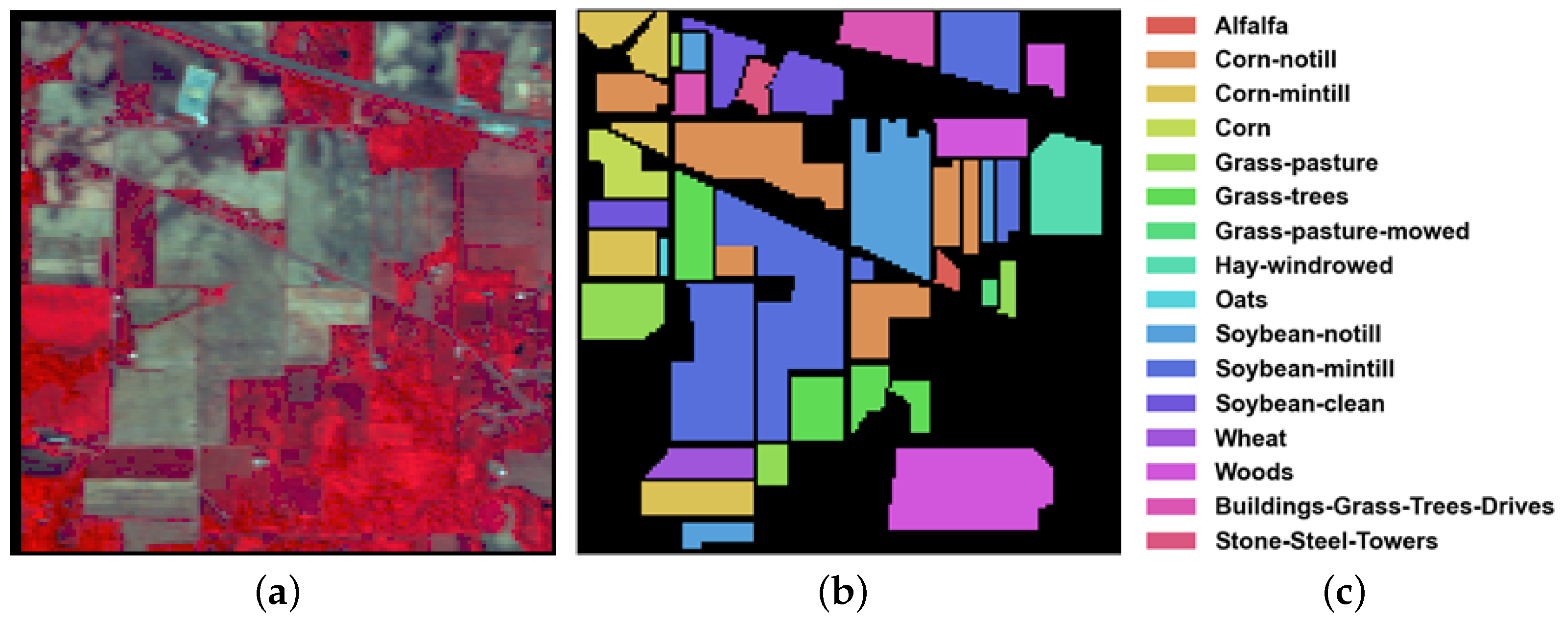
This data set was gathered by the Airborne Visible/Infrared Imaging Spectrometer (AVIRIS) sensor at a test site in northwest Indiana. It consists of 224 spectral reflectance bands in the wavelength range of 400–2500 nm. A total of 200 bands were reserved, after removing 24 invalid and corrupted bands. The image has a spatial size of 145 × 145 pixels and includes 16 mutually exclusive vegetation classes. The spatial resolution is 20 m per pixel. A false color composite, as well as detailed category descriptions and ground-truth map, are shown in Figure 3.

3.1.2. Pavia University (PU)

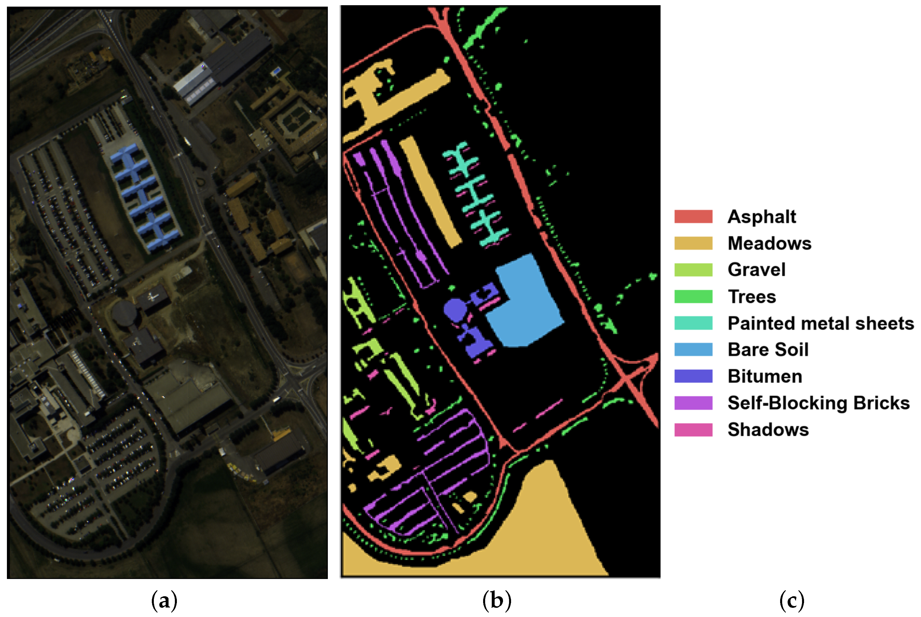
This data set was acquired by the Reflection Optical System Imaging Spectrometer (ROSIS) sensor during a flight campaign over the University of Pavia campus in northern Italy. Pavia University is a 610 × 340 pixels image with 103 spectral bands in the wavelength range of 430–860 nm. The geometric resolution is 1.3 m. This data set includes nine urban land-cover categories. A false color composite, as well as detailed category descriptions and ground truth map are shown in Figure 4.

3.1.3. Kennedy Space Center

This data set was also acquired by AVIRIS in 1996, and has a wavelength range of 400–2500 nm. The image has size of 512 × 614 pixels, and 176 bands remained after removing some low signal-to-noise ratio bands. The KSC data set includes 5202 labeled samples, with 13 upland and wetland categories. The spatial resolution is 18 m per pixel. The false color composite, with detailed category descriptions and ground truth map are shown in Figure 5.

3.2. Experimental Settings

3.2.1. Implementation Details

In order to quantify the performance of different HSIC methods, four widely used metrics were calculated, including overall accuracy (OA), Per-Class Accuracy (PA), average accuracy (AA), and Kappa coefficient. Specifically, OA is computed as the fraction of samples that are differentiated correctly, PA is the accuracy for each class, AA is calculated as the average of all per-class accuracies, and kappa coefficient is a robustness measurement considering the degree of agreement.
Regarding training details, all data sets were trained with 30 labeled pixels in each class, or 15 labeled pixels if there were less than 30 samples in the corresponding class. Network optimization was carried out using the Nesterov Adam algorithm. In addition, the learning rate and the number of training epochs were set to 0.001 and 1000, respectively. The number of superpixels N was set to 500 for the IP data set, and 1000 for the other two data sets. As for the hardware environment, our experiments were implemented in PyTorch and run on a Windows 10 machine equipped with a 3.80 GHz i7-10700K CPU, 32 GB of main memory, and an RTX 3090 GPU.

3.2.2. Compared Methods

For comparison, a number of state-of-the-art baseline methods were selected, including two conventional methods (SVM-RBF [48] and MBCTU [49]), three CNN-based methods (1D CNN [50], 2D CNN [51], and 3D CNN [52]), and three GNN-based methods (NLGCN [53], GSAGE [19], and DARMA [18]). The parameter settings for these competitors are given in the following.
1.
SVM-RBF: The value of γ (the spread of the RBF kernel) and C (controlling the magnitude of penalization) is searched in the range of γ = 2 3 , 2 3 , , 2 4 and C = 2 2 , 2 1 , , 2 4 .
2.
MBCTU: MBCTU is actually a random forest classifier that performs color-texture feature extraction based on the selected spectral bands. The bands are selected according to their feature importance computed by another random forest classifier.
3.
1D CNN: This architecture is constructed by one convolutional layer with 20 kernels, one max pooling layer, a ReLU activation layer, and two full connection layers.
4.
2D CNN: A semi-supervised classification model, consisting of one convolutional layer with a 3 × 3 filter, one max pooling layer, and followed by three decoding layers. Each decoding layer is made up of one full connection layer and one normalization layer.
5.
3D CNN: The 3D CNN model contains two convolution layers and a fully connected layer. Each convolutional layer is followed by ReLU activation layer and their kernel sizes are 3 × 3 × 7 and 3 × 3 × 3 .
6.
NLGCN: This network applies two graph convolutional layers by incorporating a graph learning procedure.
7.
GSAGE: Graph convolution is achieved by graph sampling and aggregation, and the second-order nearest neighbor of the target node is taken into account.
8.
DARMA: A superpixel-level GNN model which is composed of three convolutional blocks. Each block consists of an ARMA graph convolutional layer, a ReLU activation layer, and a normalization layer.

3.3. Experimental Results

Table 2, Table 3 and Table 4 provide information about per-class accuracies, OAs, AAs, and kappa coefficients obtained by various classification methods on the three data sets. All of the reported results were based on an average of 10 training sessions, in order to avoid bias caused by random sampling, and the top results are bolded. As is shown in the results, the two traditional methods (SVM-RBF and MBCTU) obtained similar classification results on IP and PU data sets. Due to the powerful learning ability of DL techniques, the 1D CNN, 2D CNN, and 3D CNN models outperformed the traditional classifiers. Unlike 1D CNN and 2D CNN, the 3D CNN was able to extract both spatial and spectral information at the same time, thus achieving higher classification accuracies. The Superpixel-level GNN approaches (DARMA and BKGNN), outperformed the classical machine learning, deep learning, and pixel-level GNN models. One probable explanation is that superpixel-level GNN methods exploit the latent relationship between different areas by constructing graph structures in HSI to boost classification performance, and meanwhile preserving the local spectral–spatial information through superpixel segmentation. Moreover, our method exceeded DARMA by a substantial margin on the first two data sets. This observation revealed that, compared to previous superpixel-level GNN methods, the proposed model can achieve better performance by performing adaptive feature propagation under the guidance of the homophily degree matrix. This analysis indicates the superiority of BKGNN.
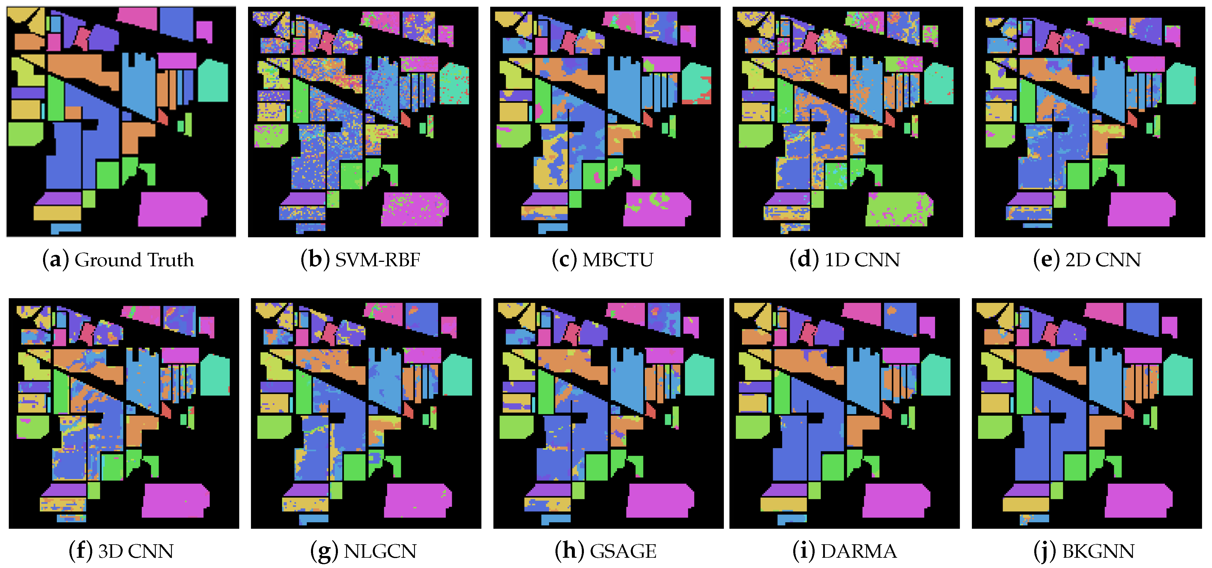
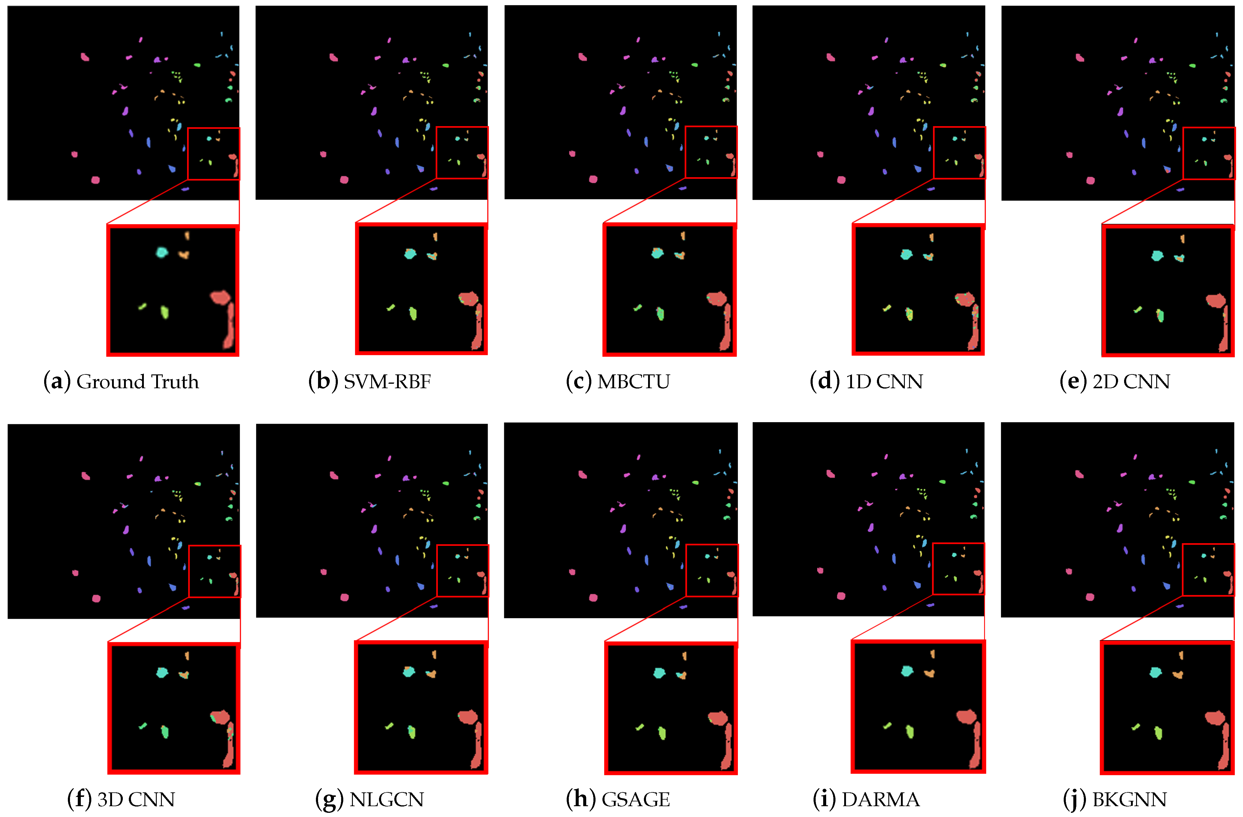
Moreover, the classification maps for the comparative methods are displayed in Figure 6, Figure 7 and Figure 8. In general, SVM-RBF and 1D CNN suffered from serious salt and pepper noise in the classification maps, while 2D CNN and 3D CNN alleviated this problem by automatically extracting spatial features. Compared with traditional classifiers and CNN-based approaches, the GNN models were able to preserve more edge details, mainly due to their ability to learn the relationships between various land-cover classes and model their spatial topologies on graphs. Compared with other methods, the visual maps of the proposed BKGNN were significantly more similar to the ground truth. This further demonstrates that the proposed model can significantly improved the discriminative ability of features to satisfy the classification performance.

4. Discussion

In this section, we analyze the influence of the number of superpixels on the effectiveness and efficiency of the proposed method, and further conduct hyper-parameter sensitivity experiments.

4.1. Analysis of the Number of Superpixels

In our proposed method, the number of superpixels N plays an important part in constructing the homophily degree matrix. We varied N from 200 to 5000, and the classification results and time costs are reported in Table 5. OM means “out of memory”. It can be seen that the OAs first grew and gradually decreased as N increased. Note that, with small N (e.g., 200), the classification accuracy was greatly reduced. This is because the superpixels might incorporate pixels with many different labels when performing superpixel segmentation. Similarly, the performance decreased with a large N, proving the importance of selecting a suitable number of superpixel for our algorithm. The number of superpixels has a significant impact on the time consumption, and a large N may even lead to out-of-memory errors. Empirically, we chose N = 500 for the IP data set, and N = 1000 for the other two data sets.

4.2. Analysis of Weights α and β

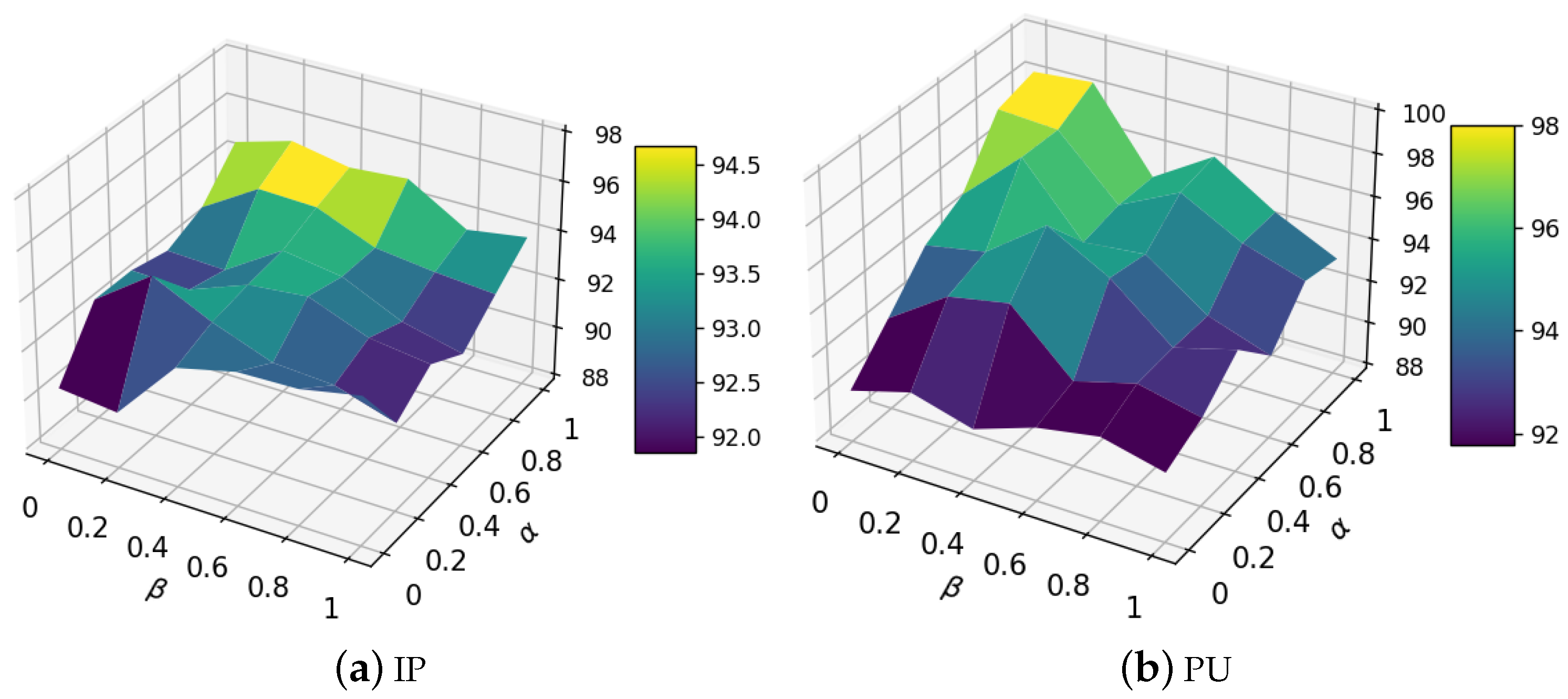
As the performance of our method highly depends on the quality of the homophily degree matrix (i.e., H ), we investigated the performance gains obtained by adjusting the two parameters α and β , which represent the weights estimated from the attribute space and topology, respectively. We show the classification performance change trend in Figure 9, obtained by varying α and β from 0 to 1. As can be seen from the figure, the performance was relatively poor when α = 0 and β = 0 , which reveals that it is necessary to estimate the homophily degree matrix by combining node attributes and network topology. Furthermore, our method performed best when α = 1 and β = 0.2 , demonstrating that the attribute information is more important than topology information on these two data sets.

4.3. Analysis of Trade-Off Parameters λ and γ

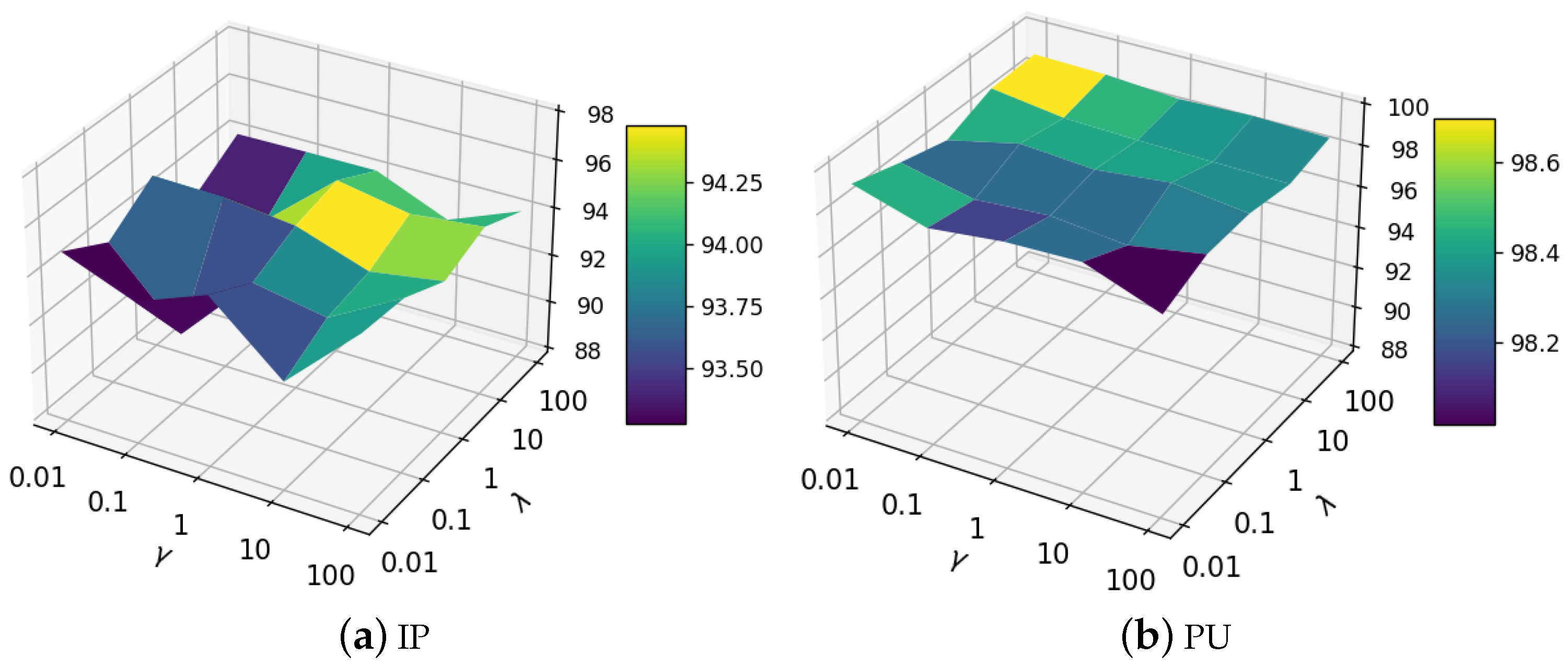
We validate our approach’s sensitivity to λ and γ which trade-off between MLP and LP loss. The value ranges of λ and γ are { 0.01 , 0.1 , 1 , 10 , 100 } . It can be seen from Figure 10a that the proposed method with parameters λ and γ in the range of 1 to 100 achieved suboptimal classification performance on the Indian Pines data set. It is interesting to observe from Figure 10b that the performance is fairly stable on the Pavia University data set. This phenomenon illustrates that the proposed BKGNN can achieve satisfactory results on a wide range of trade-off parameters, demonstrating the practicability of the algorithm.

5. Conclusions

In this paper, by analyzing the homophily levels in HSI, we find that the heterophily information that exists in the constructed graph cannot be neglected. Therefore, we propose a novel bi-kernel GNN model, which learns two kernels to model homophily and heterophily, respectively, and the kernel is adaptively selected according to a learnable homophily degree matrix. In order to better model the homophily and heterophily in graph structure, the homophily degree matrix is calculated by exploiting the topological features and attribute features through LP and MLP, respectively. The estimation of the homophily degree matrix and the process of bi-kernel feature transformation are jointly trained with supervised loss, thus they can be enhanced by each other. The experimental results on three real-world data sets demonstrated the effectiveness of our method.

Author Contributions

Conceptualization, H.H. and Y.D.; methodology, H.H.; software, H.H. and Y.D.; validation, H.H., Y.D. and F.H.; formal analysis, F.Z.; writing—original draft preparation, H.H.; writing—review and editing, Y.D., F.H. and J.Z.; visualization, F.H.; supervision, M.Y.; funding acquisition, F.Z. All authors have read and agreed to the published version of the manuscript.

Funding

This research received no external funding.

Data Availability Statement

Publicly available data sets were analyzed in this study, which can be found here: http://www.ehu.eus/ccwintco/index.php?title=Hyperspectral_Remote_Sensing_Scenes (accessed on 1 April 2022).

Acknowledgments

The authors would like to thank the authors of all the references used in the paper, the editors, and the anonymous reviewers for their detailed comments and suggestions.

Conflicts of Interest

The authors declare no conflict of interest.

References

  1. Wang, R.; Nie, F.; Yu, W. Fast spectral clustering with anchor graph for large hyperspectral images. IEEE Geosci. Remote Sens. Lett. 2017, 14, 2003–2007. [Google Scholar] [CrossRef]
  2. Chen, Y.; Lin, Z.; Zhao, X.; Wang, G.; Gu, Y. Deep learning-based classification of hyperspectral data. IEEE J. Sel. Top. Appl. Earth Obs. Remote Sens. 2014, 7, 2094–2107. [Google Scholar] [CrossRef]
  3. Bioucas-Dias, J.M.; Plaza, A.; Dobigeon, N.; Parente, M.; Du, Q.; Gader, P.; Chanussot, J. Hyperspectral unmixing overview: Geometrical, statistical, and sparse regression-based approaches. IEEE J. Sel. Top. Appl. Earth Obs. Remote Sens. 2012, 5, 354–379. [Google Scholar] [CrossRef] [Green Version]
  4. Liu, S.; Marinelli, D.; Bruzzone, L.; Bovolo, F. A review of change detection in multitemporal hyperspectral images: Current techniques, applications, and challenges. IEEE Geosci. Remote Sens. Mag. 2019, 7, 140–158. [Google Scholar] [CrossRef]
  5. Nasrabadi, N.M. Hyperspectral target detection: An overview of current and future challenges. IEEE Signal Process. Mag. 2013, 31, 34–44. [Google Scholar] [CrossRef]
  6. Li, W.; Du, Q. Collaborative representation for hyperspectral anomaly detection. IEEE Trans. Geosci. Remote Sens. 2014, 53, 1463–1474. [Google Scholar] [CrossRef]
  7. Hu, H.; Yao, M.; He, F.; Zhang, F.; Zhao, J.; Yan, S. Nonnegative collaborative representation for hyperspectral anomaly detection. Remote Sens. Lett. 2022, 13, 352–361. [Google Scholar] [CrossRef]
  8. Hu, H.; He, F.; Zhang, F.; Ding, Y.; Wu, X.; Zhao, J.; Yao, M. Unifying Label Propagation and Graph Sparsification for Hyperspectral Image Classification. IEEE Geosci. Remote Sens. Lett. 2022, 19, 1–5. [Google Scholar] [CrossRef]
  9. Blanzieri, E.; Melgani, F. Nearest Neighbor Classification of Remote Sensing Images With the Maximal Margin Principle. IEEE Trans. Geosci. Remote Sens. 2008, 46, 1804–1811. [Google Scholar] [CrossRef]
  10. Tarabalka, Y.; Fauvel, M.; Chanussot, J.; Benediktsson, J.A. SVM- and MRF-Based Method for Accurate Classification of Hyperspectral Images. IEEE Geosci. Remote Sens. Lett. 2010, 7, 736–740. [Google Scholar] [CrossRef]
  11. Fauvel, M.; Benediktsson, J.A.; Chanussot, J.; Sveinsson, J.R. Spectral and Spatial Classification of Hyperspectral Data Using SVMs and Morphological Profiles. IEEE Trans. Geosci. Remote Sens. 2008, 46, 3804–3814. [Google Scholar] [CrossRef] [Green Version]
  12. Sun, X.; Qu, Q.; Nasrabadi, N.M.; Tran, T.D. Structured Priors for Sparse-Representation-Based Hyperspectral Image Classification. IEEE Geosci. Remote Sens. Lett. 2014, 11, 1235–1239. [Google Scholar] [CrossRef] [Green Version]
  13. Uddin, M.P.; Mamun, M.A.; Hossain, M.A. Effective feature extraction through segmentation-based folded-PCA for hyperspectral image classification. Int. J. Remote Sens. 2019, 40, 7190–7220. [Google Scholar] [CrossRef]
  14. Bandos, T.V.; Bruzzone, L.; Camps-Valls, G. Classification of Hyperspectral Images With Regularized Linear Discriminant Analysis. IEEE Trans. Geosci. Remote Sens. 2009, 47, 862–873. [Google Scholar] [CrossRef]
  15. Gu, Y.; Liu, T.; Jia, X.; Benediktsson, J.A.; Chanussot, J. Nonlinear multiple kernel learning with multiple-structure-element extended morphological profiles for hyperspectral image classification. IEEE Trans. Geosci. Remote Sens. 2016, 54, 3235–3247. [Google Scholar] [CrossRef]
  16. Xia, J.; Dalla Mura, M.; Chanussot, J.; Du, P.; He, X. Random subspace ensembles for hyperspectral image classification with extended morphological attribute profiles. IEEE Trans. Geosci. Remote Sens. 2015, 53, 4768–4786. [Google Scholar] [CrossRef]
  17. Jia, S.; Hu, J.; Xie, Y.; Shen, L.; Jia, X.; Li, Q. Gabor cube selection based multitask joint sparse representation for hyperspectral image classification. IEEE Trans. Geosci. Remote Sens. 2016, 54, 3174–3187. [Google Scholar] [CrossRef]
  18. Ding, Y.; Zhao, X.; Zhang, Z.; Cai, W.; Yang, N.; Zhan, Y. Semi-Supervised Locality Preserving Dense Graph Neural Network With ARMA Filters and Context-Aware Learning for Hyperspectral Image Classification. IEEE Trans. Geosci. Remote Sens. 2021. [Google Scholar] [CrossRef]
  19. Yang, P.; Tong, L.; Qian, B.; Gao, Z.; Yu, J.; Xiao, C. Hyperspectral Image Classification With Spectral and Spatial Graph Using Inductive Representation Learning Network. IEEE J. Sel. Top. Appl. Earth Obs. Remote Sens. 2021, 14, 791–800. [Google Scholar] [CrossRef]
  20. Chen, Y.; Zhao, X.; Jia, X. Spectral–spatial classification of hyperspectral data based on deep belief network. IEEE J. Sel. Top. Appl. Earth Obs. Remote Sens. 2015, 8, 2381–2392. [Google Scholar] [CrossRef]
  21. Mou, L.; Ghamisi, P.; Zhu, X.X. Deep recurrent neural networks for hyperspectral image classification. IEEE Trans. Geosci. Remote Sens. 2017, 55, 3639–3655. [Google Scholar] [CrossRef] [Green Version]
  22. Hong, D.; Gao, L.; Yokoya, N.; Yao, J.; Chanussot, J.; Du, Q.; Zhang, B. More Diverse Means Better: Multimodal Deep Learning Meets Remote-Sensing Imagery Classification. IEEE Trans. Geosci. Remote Sens. 2021, 59, 4340–4354. [Google Scholar] [CrossRef]
  23. Hamida, A.B.; Benoit, A.; Lambert, P.; Amar, C.B. 3-D deep learning approach for remote sensing image classification. IEEE Trans. Geosci. Remote Sens. 2018, 56, 4420–4434. [Google Scholar] [CrossRef] [Green Version]
  24. Roy, S.K.; Krishna, G.; Dubey, S.R.; Chaudhuri, B.B. HybridSN: Exploring 3-D–2-D CNN feature hierarchy for hyperspectral image classification. IEEE Geosci. Remote Sens. Lett. 2019, 17, 277–281. [Google Scholar] [CrossRef] [Green Version]
  25. Zhu, K.; Chen, Y.; Ghamisi, P.; Jia, X.; Benediktsson, J.A. Deep convolutional capsule network for hyperspectral image spectral and spectral-spatial classification. Remote Sens. 2019, 11, 223. [Google Scholar] [CrossRef] [Green Version]
  26. Zhang, X.; Liang, Y.; Li, C.; Huyan, N.; Jiao, L.; Zhou, H. Recursive autoencoders-based unsupervised feature learning for hyperspectral image classification. IEEE Geosci. Remote Sens. Lett. 2017, 14, 1928–1932. [Google Scholar] [CrossRef] [Green Version]
  27. Hong, D.; Han, Z.; Yao, J.; Gao, L.; Zhang, B.; Plaza, A.; Chanussot, J. SpectralFormer: Rethinking hyperspectral image classification with transformers. IEEE Trans. Geosci. Remote Sens. 2021, 60, 1–15. [Google Scholar] [CrossRef]
  28. Bai, J.; Ding, B.; Xiao, Z.; Jiao, L.; Chen, H.; Regan, A.C. Hyperspectral Image Classification Based on Deep Attention Graph Convolutional Network. IEEE Trans. Geosci. Remote Sens. 2021. [Google Scholar] [CrossRef]
  29. Mu, C.; Dong, Z.; Liu, Y. A Two-Branch Convolutional Neural Network Based on Multi-Spectral Entropy Rate Superpixel Segmentation for Hyperspectral Image Classification. Remote Sens. 2022, 14, 1569. [Google Scholar] [CrossRef]
  30. Kipf, T.N.; Welling, M. Semi-supervised classification with graph convolutional networks. arXiv 2016, arXiv:1609.02907. [Google Scholar]
  31. Veličković, P.; Cucurull, G.; Casanova, A.; Romero, A.; Lio, P.; Bengio, Y. Graph attention networks. arXiv 2017, arXiv:1710.10903. [Google Scholar]
  32. Wang, Y.; Sun, Y.; Liu, Z.; Sarma, S.E.; Bronstein, M.M.; Solomon, J.M. Dynamic Graph CNN for Learning on Point Clouds. ACM Trans. Graph. 2019, 38, 1–12. [Google Scholar] [CrossRef]
  33. Hamilton, W.; Ying, Z.; Leskovec, J. Inductive representation learning on large graphs. Adv. Neural Inf. Process. Syst. 2017, 30, 1025–1035. [Google Scholar]
  34. Qin, A.; Shang, Z.; Tian, J.; Wang, Y.; Zhang, T.; Tang, Y.Y. Spectral Spatial Graph Convolutional Networks for Semisupervised Hyperspectral Image Classification. IEEE Geosci. Remote Sens. Lett. 2019, 16, 241–245. [Google Scholar] [CrossRef]
  35. Dong, Y.; Liu, Q.; Du, B.; Zhang, L. Weighted feature fusion of convolutional neural network and graph attention network for hyperspectral image classification. IEEE Trans. Image Process. 2022, 31, 1559–1572. [Google Scholar] [CrossRef] [PubMed]
  36. Hu, H.; Yao, M.; He, F.; Zhang, F. Graph neural network via edge convolution for hyperspectral image classification. IEEE Geosci. Remote Sens. Lett. 2021, 19, 1–5. [Google Scholar] [CrossRef]
  37. Ding, Y.; Zhao, X.; Zhang, Z.; Cai, W.; Yang, N. Graph Sample and Aggregate-Attention Network for Hyperspectral Image Classification. IEEE Geosci. Remote. Sens. Lett. 2021, 19, 5504205. [Google Scholar] [CrossRef]
  38. Ding, Y.; Zhao, X.; Zhang, Z.; Cai, W.; Yang, N. Multiscale Graph Sample and Aggregate Network With Context-Aware Learning for Hyperspectral Image Classification. IEEE J. Sel. Top. Appl. Earth Obs. Remote Sens. 2021, 14, 4561–4572. [Google Scholar] [CrossRef]
  39. Jia, S.; Deng, X.; Xu, M.; Zhou, J.; Jia, X. Superpixel-level weighted label propagation for hyperspectral image classification. IEEE Trans. Geosci. Remote Sens. 2020, 58, 5077–5091. [Google Scholar] [CrossRef]
  40. Zhang, H.; Zou, J.; Zhang, L. EMS-GCN: An End-to-End Mixhop Superpixel-Based Graph Convolutional Network for Hyperspectral Image Classification. IEEE Trans. Geosci. Remote Sens. 2022, 60, 5526116. [Google Scholar] [CrossRef]
  41. Bai, J.; Shi, W.; Xiao, Z.; Regan, A.C.; Ali, T.A.A.; Zhu, Y.; Zhang, R.; Jiao, L. Hyperspectral Image Classification Based on Superpixel Feature Subdivision and Adaptive Graph Structure. IEEE Trans. Geosci. Remote Sens. 2022, 60, 5524415. [Google Scholar] [CrossRef]
  42. Ma, Y.; Liu, X.; Shah, N.; Tang, J. Is homophily a necessity for graph neural networks? arXiv 2021, arXiv:2106.06134. [Google Scholar]
  43. Wang, T.; Jin, D.; Wang, R.; He, D.; Huang, Y. Powerful graph convolutional networks with adaptive propagation mechanism for homophily and heterophily. In Proceedings of the AAAI Conference on Artificial Intelligence, Virtual, 22 February– 1 March 2022; Volume 36, pp. 4210–4218. [Google Scholar]
  44. Zhu, J.; Yan, Y.; Zhao, L.; Heimann, M.; Akoglu, L.; Koutra, D. Beyond homophily in graph neural networks: Current limitations and effective designs. Adv. Neural Inf. Process. Syst. 2020, 33, 7793–7804. [Google Scholar]
  45. Gilmer, J.; Schoenholz, S.S.; Riley, P.F.; Vinyals, O.; Dahl, G.E. Neural message passing for quantum chemistry. In Proceedings of the International Conference on Machine Learning, PMLR, Sydney, Australia, 6–11 August 2017; pp. 1263–1272. [Google Scholar]
  46. Li, G.; Mueller, M.; Qian, G.; Delgadillo Perez, I.C.; Abualshour, A.; Thabet, A.K.; Ghanem, B. DeepGCNs: Making GCNs Go as Deep as CNNs. IEEE Trans. Pattern Anal. Mach. Intell. 2021. [Google Scholar] [CrossRef] [PubMed]
  47. Du, L.; Shi, X.; Fu, Q.; Ma, X.; Liu, H.; Han, S.; Zhang, D. GBK-GNN: Gated Bi-Kernel Graph Neural Networks for Modeling Both Homophily and Heterophily. In Proceedings of the ACM Web Conference 2022, Virtual Event, 25–29 April 2022; pp. 1550–1558. [Google Scholar]
  48. Kuo, B.C.; Ho, H.H.; Li, C.H.; Hung, C.C.; Taur, J.S. A kernel-based feature selection method for SVM with RBF kernel for hyperspectral image classification. IEEE J. Sel. Top. Appl. Earth Obs. Remote Sens. 2013, 7, 317–326. [Google Scholar] [CrossRef]
  49. Djerriri, K.; Safia, A.; Adjoudj, R.; Karoui, M.S. Improving hyperspectral image classification by combining spectral and multiband compact texture features. In Proceedings of the IGARSS 2019—2019 IEEE International Geoscience and Remote Sensing Symposium, Yokohama, Japan, 28 July–2 August 2019; pp. 465–468. [Google Scholar]
  50. Hu, W.; Huang, Y.; Wei, L.; Zhang, F.; Li, H. Deep convolutional neural networks for hyperspectral image classification. J. Sens. 2015, 2015, 258619. [Google Scholar] [CrossRef] [Green Version]
  51. Liu, B.; Yu, X.; Zhang, P.; Tan, X.; Yu, A.; Xue, Z. A semi-supervised convolutional neural network for hyperspectral image classification. Remote Sens. Lett. 2017, 8, 839–848. [Google Scholar] [CrossRef]
  52. Li, Y.; Zhang, H.; Shen, Q. Spectral–spatial classification of hyperspectral imagery with 3D convolutional neural network. Remote Sens. 2017, 9, 67. [Google Scholar] [CrossRef] [Green Version]
  53. Mou, L.; Lu, X.; Li, X.; Zhu, X.X. Nonlocal Graph Convolutional Networks for Hyperspectral Image Classification. IEEE Trans. Geosci. Remote Sens. 2020, 58, 8246–8257. [Google Scholar] [CrossRef]
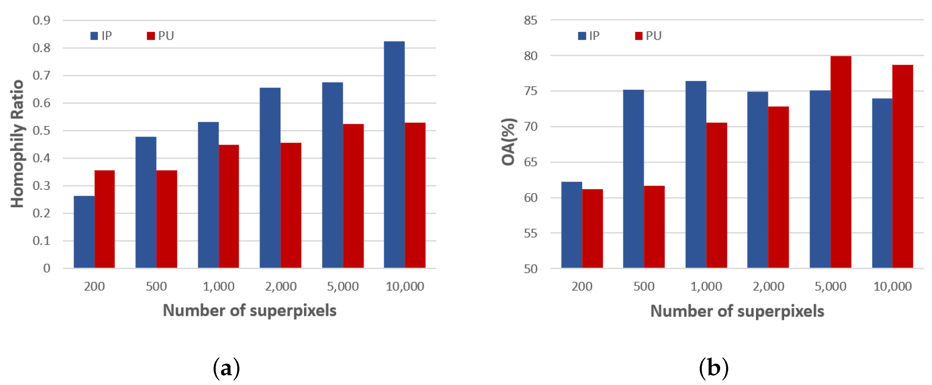
Figure 1. (a) Homophily Ratio and (b) overall accuracy (OA) with different number of superpixels on Indian Pines (IP) and Pavia University (PU) data sets.
Remotesensing 14 06224 g001
Figure 2. Overview of BKGNN. BKGNN has four main modules: Graph projection, homophily degree matrix estimation, bi-kernel feature transformation, and graph re-projection. The first module maps the original pixel-level HSI data to a superpixel-level graph structure, after which the homophily degree matrix is learned from the attribute and topological information, which is further used to conduct the bi-kernel feature transformation for capturing the similarity between nodes and the dissimilarity between nodes. After graph re-projection, the pixel-level result is obtained.
Remotesensing 14 06224 g002
Figure 3. IP data set: (a) False color image; (b) Ground truth map; and (c) Color bar.
Remotesensing 14 06224 g003
Figure 4. PU data set: (a) False color image; (b) Ground truth map; and (c) Color bar.
Remotesensing 14 06224 g004
Figure 5. KSC data set: (a) False color image; (b) Ground truth map; and (c) Color bar.
Remotesensing 14 06224 g005
Figure 6. Ground truth and classification maps obtained by different methods on the Indian Pines data set.
Remotesensing 14 06224 g006
Figure 7. Ground truth and classification maps obtained by different methods on the Pavia University data set.
Remotesensing 14 06224 g007
Figure 8. Ground truth and classification maps obtained by different methods on the Kennedy Space Center data set.
Remotesensing 14 06224 g008
Figure 9. Analysis results for varying weights α and β .
Remotesensing 14 06224 g009
Figure 10. Analysis results of trade-off parameters λ and γ .
Remotesensing 14 06224 g010
Table 1. Main notation and descriptions.
NotationDefinitionTypeSize
X Original HSI data.3D matrix H × W × B
H, W and BHeight, width, and number of bands in HSI, respectively.Scalar 1 × 1
CNumber of classes in HSI.Scalar 1 × 1
NNumber of nodes contained in the graph (equal to the number of superpixels).Scalar 1 × 1
G = ( V , E ) Graph G with node set V and edge set E .--
A Adjacency matrix.Matrix N × N
V Attribute matrix.Matrix N × B
D Degree matrix of A .Matrix N × N
Q , Q ^ Projection matrix and its normalized version.Matrix H W × B
H Homophily degree matrixMatrix N × N
Z Node embeddingsMatrix N × F
S i The set of pixels in the i th superpixel.--
N ( · ) Neighborhood of ·.--
T V Nodes in the training set.--
Table 2. Accuracy comparison for the IP data set. Bold numbers indicate the best performance.
Class
No.
Conventional ClassifiersCNN-Based MethodsGNN-Based Methods
SVM-RBFMBCTU1D CNN2D CNN3D CNNNLGCNGSAGEDARMABKGNN
187.50 ± 5.1095.83 ± 2.9596.25 ± 4.1597.50 ± 4.1599.38 ± 1.8798.75 ± 2.50100.00 ± 0.00100.00 ± 0.00100.00 ± 0.00
255.74 ± 3.9947.76 ± 0.6563.21 ± 6.7858.06 ± 9.1366.82 ± 7.5874.93 ± 8.2276.02 ± 6.5380.07 ± 6.1588.54 ± 2.34
358.66 ± 4.3268.17 ± 4.2569.05 ± 7.3749.59 ± 6.1658.53 ± 5.0478.56 ± 3.5970.30 ± 9.8694.07 ± 3.3294.68 ± 3.18
470.53 ± 8.1598.87 ± 0.9186.04 ± 6.7683.14 ± 5.0284.69 ± 4.5092.08 ± 3.7397.49 ± 1.6199.61 ± 0.36100.00 ± 0.00
584.32 ± 4.6771.52 ± 7.1973.95 ± 16.5877.15 ± 6.7887.24 ± 3.6793.11 ± 2.1791.30 ± 9.1095.01 ± 2.1296.25 ± 2.60
690.61 ± 2.1386.68 ± 0.5391.27 ± 3.6295.61 ± 2.4891.87 ± 3.1996.96 ± 2.3397.71 ± 2.6096.51 ± 0.7198.83 ± 1.21
790.74 ± 6.92100.00 ± 0.0086.92 ± 7.7396.15 ± 7.0998.46 ± 3.0897.69 ± 4.9398.46 ± 4.6296.92 ± 3.77100.00 ± 0.00
889.58 ± 3.0186.53 ± 5.5594.58 ± 1.7898.57 ± 0.8097.05 ± 1.3599.67 ± 0.3097.90 ± 4.6399.51 ± 0.78100.00 ± 0.00
996.66 ± 4.7193.33 ± 9.4398.00 ± 6.00100.00 ± 0.00100.00 ± 0.00100.00 ± 0.0082.00 ± 32.80100.00 ± 0.00100.00 ± 0.00
1070.24 ± 2.8686.13 ± 6.0770.91 ± 7.6875.34 ± 5.2372.46 ± 8.0287.58 ± 3.4286.28 ± 8.7789.07 ± 2.9793.48 ± 3.00
1150.59 ± 3.7260.89 ± 9.6463.65 ± 7.9163.56 ± 7.2566.19 ± 5.1571.95 ± 4.1067.46 ± 6.2586.95 ± 4.3692.17 ± 3.74
1262.87 ± 6.5252.46 ± 13.0870.55 ± 8.7567.41 ± 9.4572.02 ± 6.5989.17 ± 2.6486.77 ± 7.5589.66 ± 4.4196.45 ± 1.00
1396.57 ± 0.9399.43 ± 0.2596.63 ± 1.9099.89 ± 0.3499.20 ± 0.7899.49 ± 0.4099.83 ± 0.2699.89 ± 0.23100.00 ± 0.00
1482.37 ± 3.9786.23 ± 1.0383.28 ± 11.1390.95 ± 5.5690.87 ± 3.5191.07 ± 2.8295.51 ± 3.1097.51 ± 2.6798.17 ± 1.99
1564.04 ± 2.9874.44 ± 4.2558.62 ± 12.5061.74 ± 6.2267.42 ± 9.7588.01 ± 5.9593.12 ± 3.1298.43 ± 1.6199.72 ± 0.36
1689.41 ± 8.3399.47 ± 0.7594.29 ± 4.0399.68 ± 0.9598.41 ± 2.56100.00 ± 0.00100.00 ± 0.00100.00 ± 0.00100.00 ± 0.00
OA66.93 ± 1.5070.62 ± 2.9472.64 ± 2.4172.31 ± 1.0775.27 ± 1.1183.62 ± 1.7282.48 ± 2.2290.91 ± 2.4294.66 ± 0.91
AA77.53 ± 1.4681.75 ± 2.1781.07 ± 1.1882.15 ± 1.3884.41 ± 1.1491.19 ± 0.9790.01 ± 2.5695.20 ± 1.3597.39 ± 0.31
Kappa62.81 ± 1.6666.83 ± 3.2869.04 ± 2.6468.76 ± 1.1271.98 ± 1.2681.44 ± 1.9380.16 ± 2.4889.62 ± 2.7693.90 ± 1.03
Table 3. Accuracy comparison for the PU data set. Bold numbers indicate the best performance.
Class
No.
Conventional ClassifiersCNN-Based MethodsGNN-Based Methods
SVM-RBFMBCTU1D CNN2D CNN3D CNNNLGCNGSAGEDARMABKGNN
165.14 ± 5.4575.89 ± 4.6469.58 ± 4.0066.94 ± 8.5075.56 ± 11.8588.30 ± 2.6090.54 ± 3.0194.03 ± 1.3596.76 ± 0.72
259.19 ± 4.4555.52 ± 14.5665.41 ± 13.7061.68 ± 4.4974.15 ± 11.4175.17 ± 7.5481.87 ± 6.9590.75 ± 5.5398.62 ± 1.21
327.69 ± 2.4666.30 ± 7.3568.27 ± 23.9262.24 ± 15.6181.08 ± 8.3489.70 ± 1.8288.09 ± 8.4895.90 ± 5.0999.40 ± 0.77
495.25 ± 2.1492.23 ± 1.7593.84 ± 4.3291.80 ± 2.0591.14 ± 3.9694.18 ± 1.7894.74 ± 2.6088.49 ± 3.0196.86 ± 1.13
599.18 ± 0.14100.00 ± 0.0099.41 ± 0.2099.38 ± 0.4198.82 ± 0.5999.69 ± 0.22100.00 ± 0.0097.83 ± 0.8499.68 ± 0.42
670.42 ± 9.4970.01 ± 20.6359.33 ± 17.9882.68 ± 5.2367.06 ± 18.2780.53 ± 6.4289.98 ± 5.6294.94 ± 4.7299.82 ± 0.17
790.10 ± 1.4595.82 ± 1.5391.74 ± 1.4785.19 ± 7.8890.48 ± 2.9296.15 ± 0.6296.95 ± 2.6099.91 ± 0.06100.00 ± 0.00
887.03 ± 2.8177.99 ± 11.5071.60 ± 17.1272.50 ± 12.9692.27 ± 4.7792.83 ± 2.7386.19 ± 9.4895.35 ± 1.6898.96 ± 0.51
999.92 ± 0.0598.80 ± 0.2799.95 ± 0.0599.13 ± 0.5198.52 ± 0.7799.97 ± 0.0599.96 ± 0.0596.53 ± 1.9397.71 ± 2.05
OA67.93 ± 0.5569.01 ± 4.2070.65 ± 4.8270.77 ± 2.5078.43 ± 3.1183.36 ± 3.2287.17 ± 3.1692.86 ± 2.6298.47 ± 0.58
AA77.11 ± 0.1681.40 ± 1.1779.90 ± 1.4780.17 ± 1.7485.45 ± 1.6790.72 ± 1.0192.03 ± 1.0694.86 ± 1.3798.65 ± 0.27
Kappa60.27 ± 0.2561.86 ± 3.9763.18 ± 4.9463.96 ± 2.7472.59 ± 3.2878.80 ± 3.8383.58 ± 3.8190.69 ± 3.3197.98 ± 0.76
Table 4. Accuracy comparison for the KSC data set. Bold numbers indicate the best performance.
Class
No.
Conventional ClassifiersCNN-Based MethodsGNN-Based Methods
SVM-RBFMBCTU1D CNN2D CNN3D CNNNLGCNGSAGEDARMABKGNN
189.78 ± 1.8997.84 ± 0.1079.78 ± 17.2979.49 ± 5.5593.57 ± 6.1697.13 ± 1.2696.79 ± 2.0099.64 ± 0.2499.97 ± 0.05
284.66 ± 0.5892.49 ± 2.2683.90 ± 4.0880.85 ± 11.1474.65 ± 7.8690.94 ± 2.4691.92 ± 2.1297.28 ± 3.15100.00 ± 0.00
356.78 ± 22.2194.87 ± 2.1450.44 ± 34.2469.03 ± 17.8685.40 ± 12.6794.65 ± 5.3297.92 ± 5.6697.26 ± 2.3099.82 ± 0.22
426.42 ± 19.2314.14 ± 4.6332.93 ± 23.1646.08 ± 14.7522.52 ± 13.8059.46 ± 9.5454.23 ± 23.7499.01 ± 1.4198.65 ± 1.61
538.42 ± 2.0044.43 ± 5.6638.93 ± 13.5666.26 ± 13.7584.73 ± 5.6785.65 ± 8.6184.89 ± 18.6387.79 ± 0.8496.34 ± 2.95
641.37 ± 2.4777.69 ± 1.2938.89 ± 11.6680.65 ± 15.1179.90 ± 9.2475.58 ± 8.8587.04 ± 6.5997.59 ± 4.11100.00 ± 0.00
789.33 ± 2.1795.47 ± 4.2784.67 ± 16.4495.33 ± 8.5698.00 ± 1.5495.20 ± 6.0998.27 ± 3.16100.00 ± 0.0099.47 ± 1.07
844.80 ± 8.0365.34 ± 4.1483.44 ± 6.9567.88 ± 5.0569.58 ± 4.1793.17 ± 2.9397.33 ± 2.50100.00 ± 0.00100.00 ± 0.00
975.98 ± 6.6783.43 ± 1.1371.94 ± 16.7184.02 ± 5.7781.63 ± 8.7496.88 ± 4.4997.14 ± 2.66100.00 ± 0.00100.00 ± 0.00
1065.95 ± 1.8193.64 ± 2.6778.66 ± 8.9996.47 ± 2.6194.92 ± 3.7697.99 ± 1.6196.39 ± 5.7999.79 ± 0.1199.89 ± 0.13
1189.88 ± 1.15100.00 ± 0.0093.42 ± 1.3999.54 ± 0.5299.74 ± 1.6598.92 ± 0.94100.00 ± 0.00100.00 ± 0.00100.00 ± 0.00
1283.72 ± 2.1089.81 ± 0.8480.13 ± 4.9594.28 ± 4.8782.47 ± 1.8192.79 ± 3.2195.03 ± 3.2899.37 ± 1.2799.20 ± 1.50
1399.85 ± 0.14100.00 ± 0.00100.00 ± 0.0099.99 ± 0.03100.00 ± 0.0099.79 ± 0.46100.00 ± 0.00100.00 ± 0.00100.00 ± 0.00
OA75.98 ± 0.3186.58 ± 0.3478.03 ± 4.3384.18 ± 1.9385.87 ± 1.6493.70 ± 0.7394.70 ± 1.3199.14 ± 0.4199.73 ± 0.14
AA68.23 ± 0.1580.70 ± 0.5570.55 ± 4.2179.86 ± 2.9782.24 ± 2.8090.63 ± 1.1192.07 ± 1.6098.29 ± 0.5899.49 ± 0.26
Kappa73.14 ± 0.3484.99 ± 0.3875.53 ± 4.7482.38 ± 2.1584.22 ± 1.9492.95 ± 0.8194.08 ± 1.4799.04 ± 0.4599.70 ± 0.16
Table 5. Classification performance (OA) and time cost (s) with varying N on three data sets.
Datasets20050010002000300040005000
IPOA89.6594.6694.5992.7091.9491.5590.25
time18.721.224.870.476.71339.1342.8
PUOA90.2597.6698.4795.7897.6996.1094.68
time45.050.866.2104.1185.4301.1OM
KSCOA95.5798.7499.7399.6098.1898.3798.47
time69.974.789.5125.9216.5285.5OM
Publisher’s Note: MDPI stays neutral with regard to jurisdictional claims in published maps and institutional affiliations.