


Semantic Segmentation for Digital Archives of Borobudur Reliefs Based on Soft-Edge Enhanced Deep Learning
 ,
,
Abstract
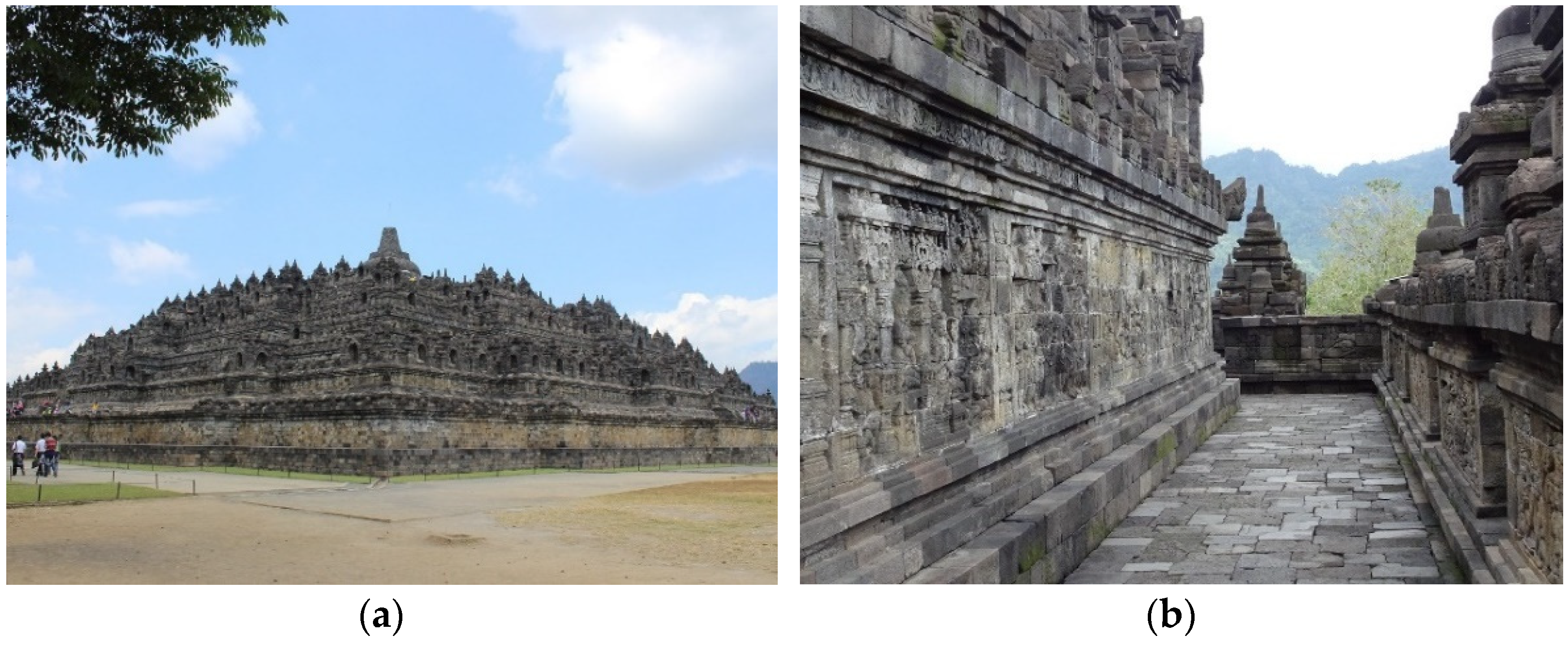
1. Introduction
2. Related Work
3. Method
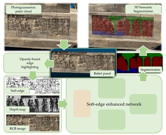
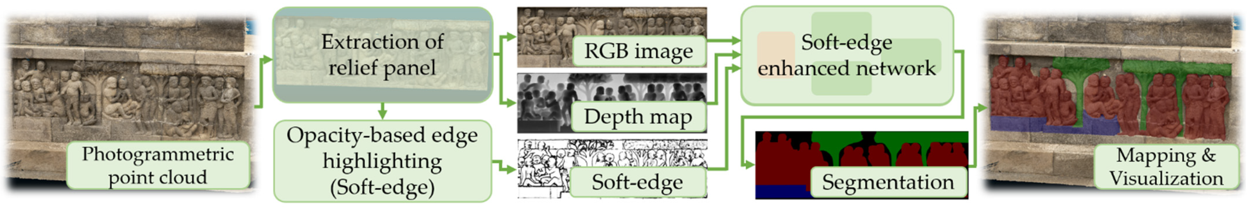
3.1. Overview
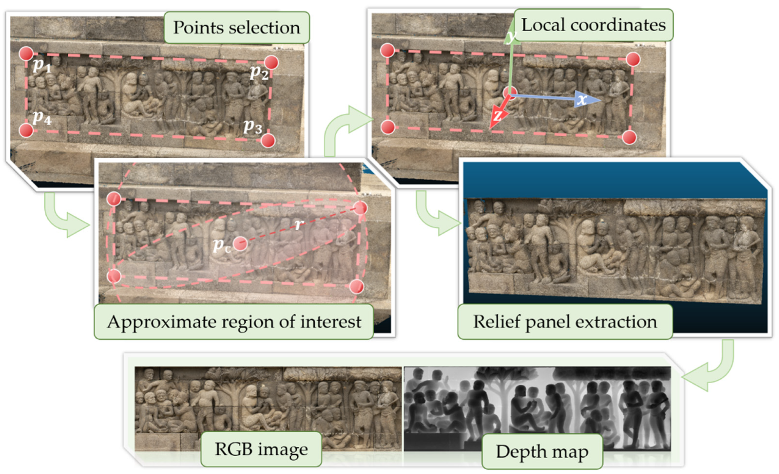
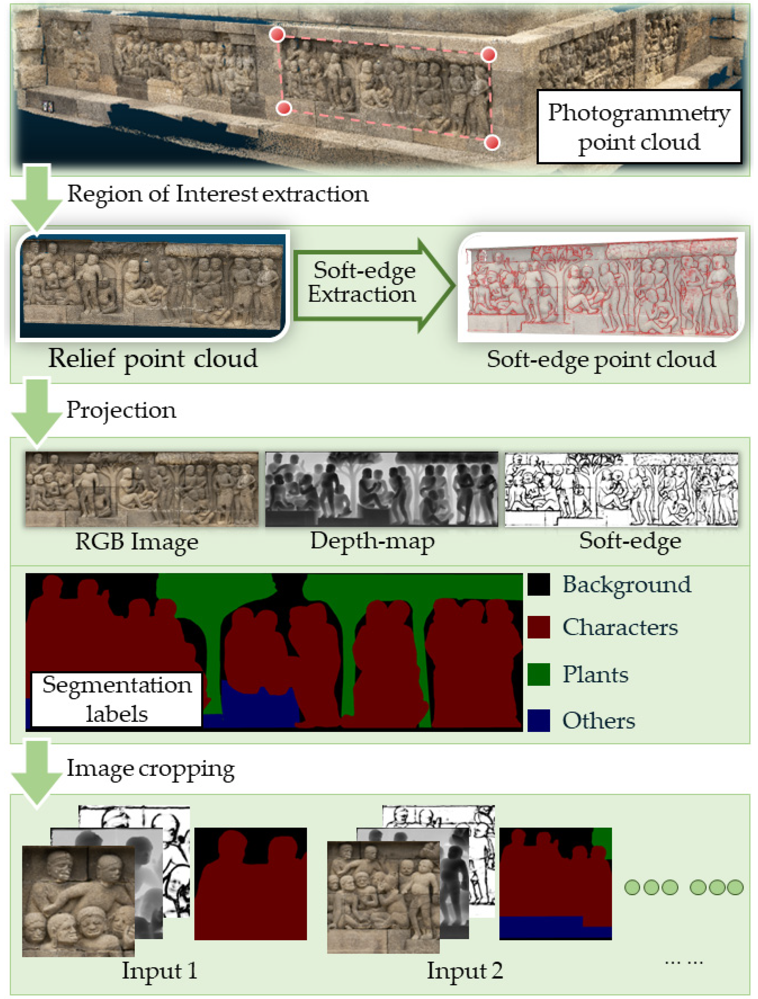
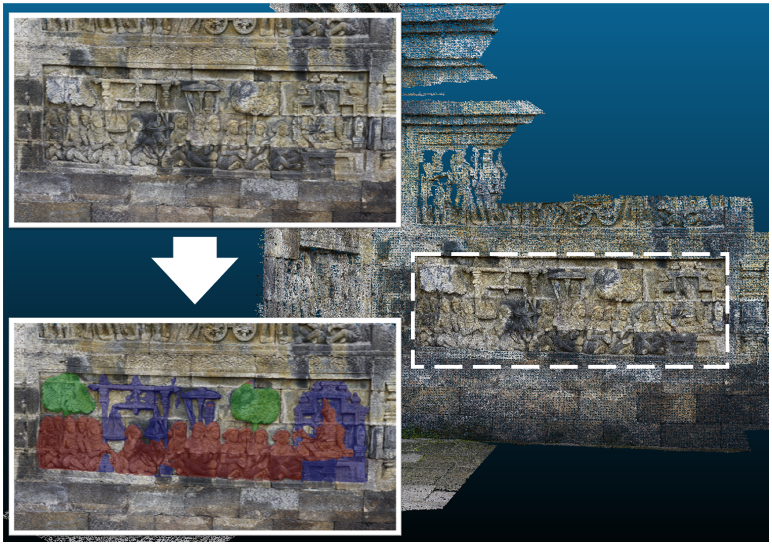
3.2. Relief Panel Extraction and RGB-D Image Projection
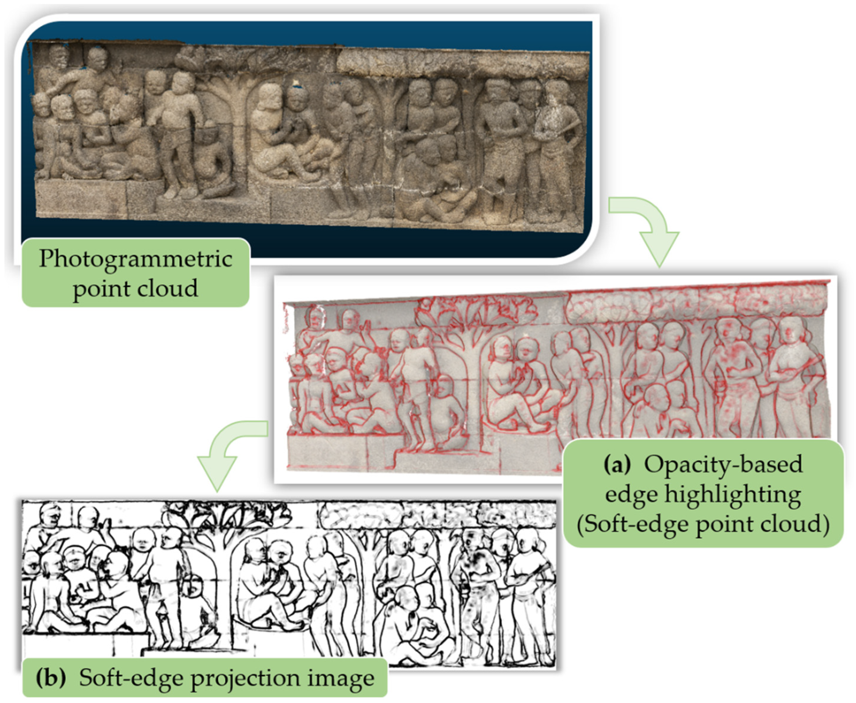
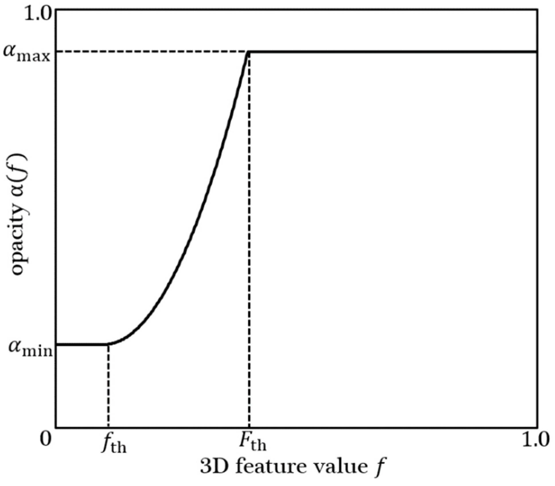
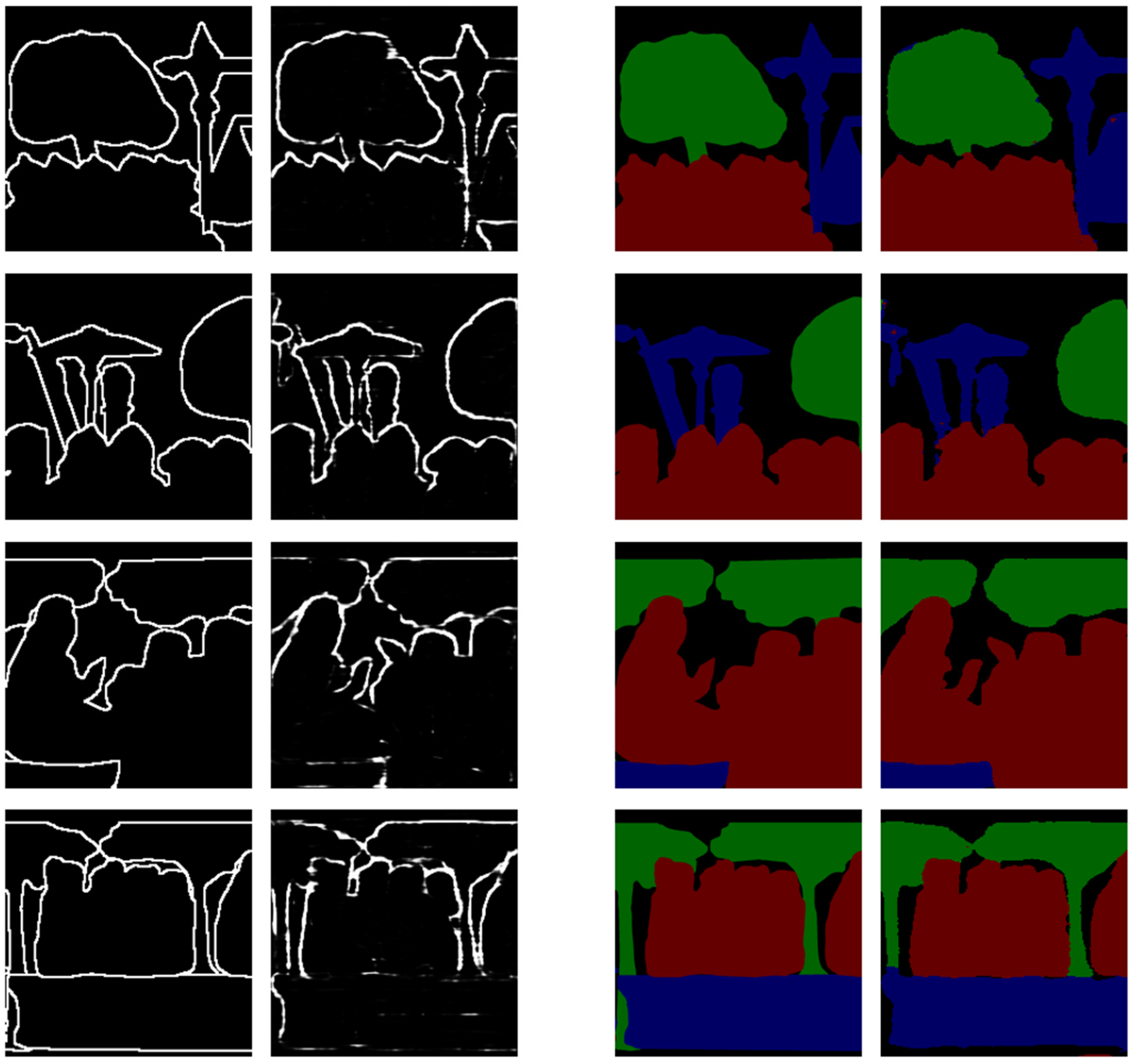
3.3. Opacity-Based Edge Highlighting
3.4. Soft-Edge Enhanced Network for Semantic Segmentation
3.4.1. Soft-Edge Enhanced Utilization
3.4.2. Network Structure
3.4.3. Training Loss
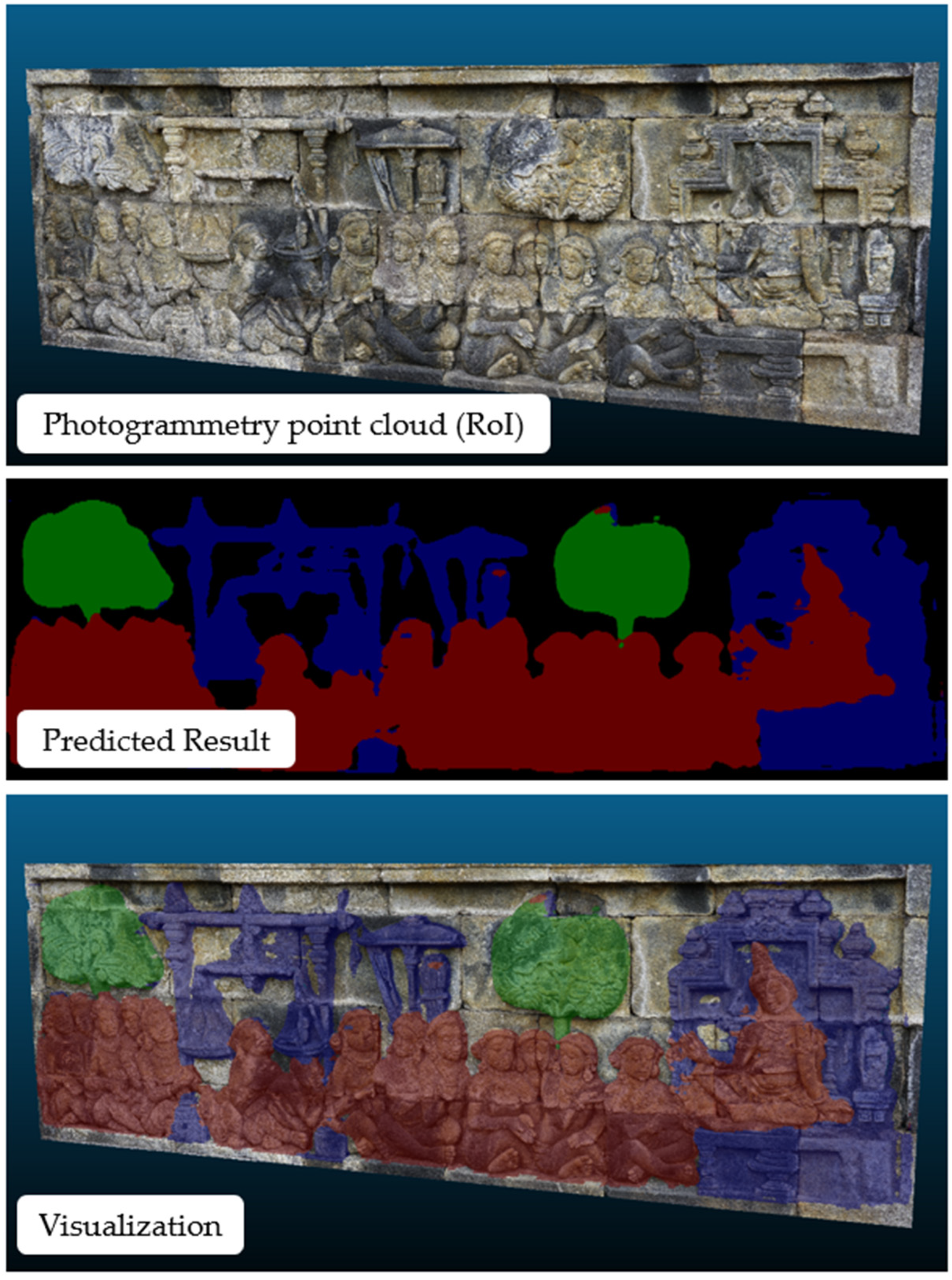
3.5. Mapping and Visualization
4. Experimental Results
4.1. Dataset Creation
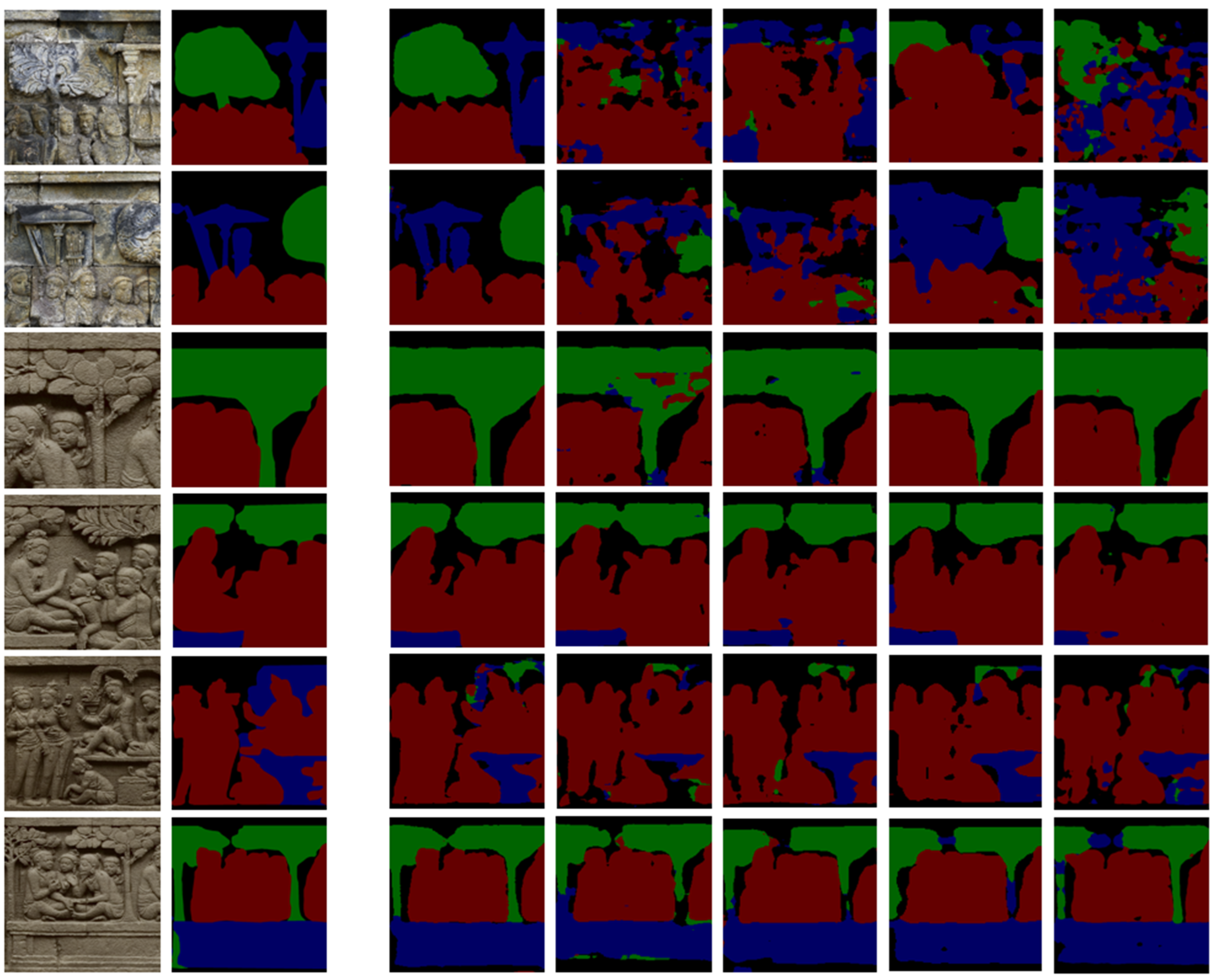
4.2. Network Evaluation
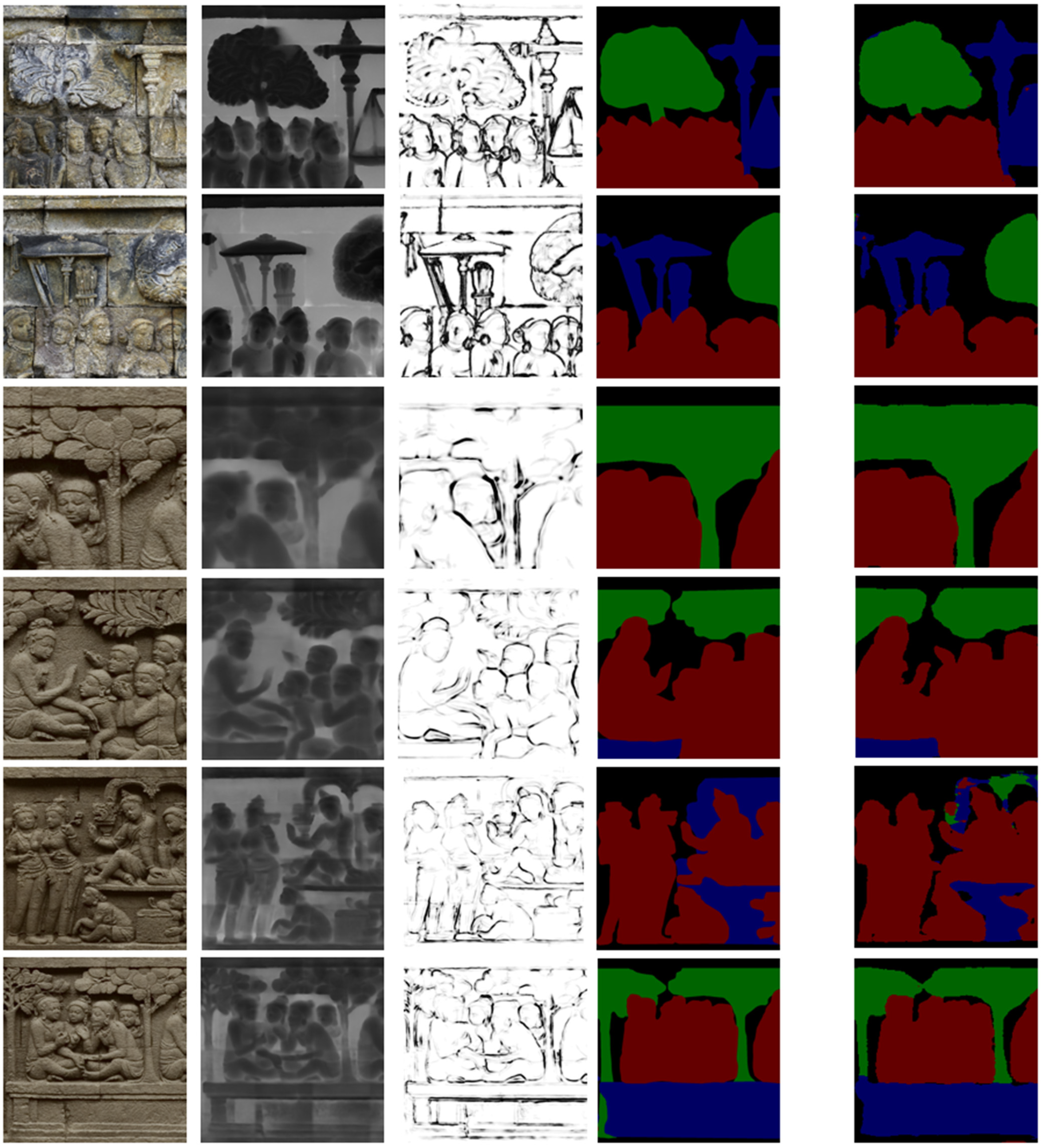
4.3. Visualization Results
5. Discussion
6. Conclusions
Author Contributions
Funding
Data Availability Statement
Acknowledgments
Conflicts of Interest
References
- Pavlidis, G.; Koutsoudis, A.; Arnaoutoglou, F.; Tsioukas, V.; Chamzas, C. Methods for 3D Digitization of Cultural Heritage. J. Cult. Herit. 2007, 8, 93–98. [Google Scholar]
- Pieraccini, M.; Guidi, G.; Atzeni, C. 3D Digitizing of Cultural Heritage. J. Cult. Herit. 2001, 2, 63–70. [Google Scholar]
- Li, R.; Luo, T.; Zha, H. 3D Digitization and Its Applications in Cultural Heritage. In Proceedings of the Euro-Mediterranean Conference, Lemesos, Cyprus, 8–13 November 2010; pp. 381–388. [Google Scholar]
- Barsanti, G.; Remondino, F.; Palacios, J.F. Critical Factors and Guidelines for 3D Surveying and Modelling in Cultural Heritage. Int. J. Herit. Digit. Era 2014, 3, 141–158. [Google Scholar]
- Kingsland, K. Comparative Analysis of Digital Photogrammetry Software for Cultural Heritage. Digit. Appl. Archaeol. Cult. Herit. 2020, 18, e00157. [Google Scholar] [CrossRef]
- Barsanti, S.G.; Guidi, G. A New Methodology for the Structural Analysis of 3D Digitized Cultural Heritage through FEA. IOP Conf. Ser. Mater. Sci. Eng. 2018, 364, 12005. [Google Scholar] [CrossRef]
- Doulamis, N.; Doulamis, A.; Ioannidis, C.; Klein, M.; Ioannides, M. Modelling of Static and Moving Objects: Digitizing Tangible and Intangible Cultural Heritage. In Mixed Reality and Gamification for Cultural Heritage; Springer: Berlin/Heidelberg, Germany, 2017; pp. 567–589. [Google Scholar]
- Wu, B.; Wan, A.; Yue, X.; Keutzer, K. Squeezeseg: Convolutional Neural Nets with Recurrent Crf for Real-Time Road-Object Segmentation from 3d Lidar Point Cloud. In Proceedings of the 2018 IEEE International Conference on Robotics and Automation (ICRA), Brisbane, Australia, 21–25 May 2018; pp. 1887–1893. [Google Scholar]
- Zhou, D.; Fang, J.; Song, X.; Liu, L.; Yin, J.; Dai, Y.; Li, H.; Yang, R. Joint 3D Instance Segmentation and Object Detection for Autonomous Driving. In Proceedings of the IEEE/CVF Conference on Computer Vision and Pattern Recognition, Seattle, WA, USA, 13–19 June 2020; pp. 1839–1849. [Google Scholar]
- el Madawi, K.; Rashed, H.; el Sallab, A.; Nasr, O.; Kamel, H.; Yogamani, S. Rgb and Lidar Fusion Based 3d Semantic Segmentation for Autonomous Driving. In Proceedings of the 2019 IEEE Intelligent Transportation Systems Conference (ITSC), Auckland, NZ, USA, 27–30 October 2019; pp. 7–12. [Google Scholar]
- Biasutti, P.; Lepetit, V.; Aujol, J.-F.; Brédif, M.; Bugeau, A. Lu-Net: An Efficient Network for 3d Lidar Point Cloud Semantic Segmentation Based on End-to-End-Learned 3d Features and u-Net. In Proceedings of the IEEE/CVF International Conference on Computer Vision Workshops, Seoul, Republic of Korea, 27–28 October 2019; pp. 942–950. [Google Scholar]
- Bogoslavskyi, I.; Stachniss, C. Fast Range Image-Based Segmentation of Sparse 3D Laser Scans for Online Operation. In Proceedings of the 2016 IEEE/RSJ International Conference on Intelligent Robots and Systems (IROS), Daejeon, Republic of Korea, 9–14 October 2016; pp. 163–169. [Google Scholar]
- Penza, V.; Ortiz, J.; Mattos, L.S.; Forgione, A.; de Momi, E. Dense Soft Tissue 3D Reconstruction Refined with Super-Pixel Segmentation for Robotic Abdominal Surgery. Int. J. Comput. Assist. Radiol. Surg. 2016, 11, 197–206. [Google Scholar] [PubMed]
- Su, Y.-H.; Huang, I.; Huang, K.; Hannaford, B. Comparison of 3d Surgical Tool Segmentation Procedures with Robot Kinematics Prior. In Proceedings of the 2018 IEEE/RSJ International Conference on Intelligent Robots and Systems (IROS), Madrid, Spain, 1–5 October 2018; pp. 4411–4418. [Google Scholar]
- Pierdicca, R.; Paolanti, M.; Matrone, F.; Martini, M.; Morbidoni, C.; Malinverni, E.S.; Frontoni, E.; Lingua, A.M. Point Cloud Semantic Segmentation Using a Deep Learning Framework for Cultural Heritage. Remote Sens. 2020, 12, 1005. [Google Scholar]
- Grilli, E.; Remondino, F. Classification of 3D Digital Heritage. Remote Sens. 2019, 11, 847. [Google Scholar]
- Matrone, F.; Grilli, E.; Martini, M.; Paolanti, M.; Pierdicca, R.; Remondino, F. Comparing Machine and Deep Learning Methods for Large 3D Heritage Semantic Segmentation. ISPRS Int. J. Geoinf. 2020, 9, 535. [Google Scholar]
- Mathias, M.; Martinovic, A.; Weissenberg, J.; Haegler, S.; van Gool, L. Automatic Architectural Style Recognition. ISPRS-Int. Arch. Photogramm. Remote Sens. Spat. Inf. Sci. 2011, 3816, 171–176. [Google Scholar] [CrossRef]
- Oses, N.; Dornaika, F.; Moujahid, A. Image-Based Delineation and Classification of Built Heritage Masonry. Remote Sens. 2014, 6, 1863–1889. [Google Scholar] [CrossRef]
- Shalunts, G.; Haxhimusa, Y.; Sablatnig, R. Architectural Style Classification of Building Facade Windows. In Proceedings of the International Symposium on Visual Computing, Las Vegas, NV, USA, 26–28 September 2011; pp. 280–289. [Google Scholar]
- Zhang, L.; Song, M.; Liu, X.; Sun, L.; Chen, C.; Bu, J. Recognizing Architecture Styles by Hierarchical Sparse Coding of Blocklets. Inf. Sci. 2014, 254, 141–154. [Google Scholar] [CrossRef]
- Llamas, J.; Lerones, P.M.; Medina, R.; Zalama, E.; Gómez-García-Bermejo, J. Classification of Architectural Heritage Images Using Deep Learning Techniques. Appl. Sci. 2017, 7, 992. [Google Scholar]
- Qi, C.R.; Su, H.; Mo, K.; Guibas, L.J. Pointnet: Deep Learning on Point Sets for 3d Classification and Segmentation. In Proceedings of the IEEE Conference on Computer Vision and Pattern Recognition, Honolulu, HI, USA, 21–26 July 2017; pp. 652–660. [Google Scholar]
- Qi, C.R.; Yi, L.; Su, H.; Guibas, L.J. Pointnet++: Deep Hierarchical Feature Learning on Point Sets in a Metric Space. Adv. Neural. Inf. Process. Syst. 2017, 30, 5105–5114. [Google Scholar]
- Wu, W.; Qi, Z.; Fuxin, L. Pointconv: Deep Convolutional Networks on 3d Point Clouds. In Proceedings of the IEEE/CVF Conference on Computer Vision and Pattern Recognition, Long Beach, CA, USA, 15–20 June 2019; pp. 9621–9630. [Google Scholar]
- Wang, Y.; Sun, Y.; Liu, Z.; Sarma, S.E.; Bronstein, M.M.; Solomon, J.M. Dynamic Graph Cnn for Learning on Point Clouds. ACM Trans. Graph. 2019, 38, 1–12. [Google Scholar] [CrossRef]
- Thomas, H.; Qi, C.R.; Deschaud, J.-E.; Marcotegui, B.; Goulette, F.; Guibas, L.J. Kpconv: Flexible and Deformable Convolution for Point Clouds. In Proceedings of the IEEE/CVF International Conference on Computer Vision, Seoul, Republic of Korea, 27 October–2 November 2019; pp. 6411–6420. [Google Scholar]
- Hua, B.-S.; Tran, M.-K.; Yeung, S.-K. Pointwise Convolutional Neural Networks. In Proceedings of the IEEE Conference on Computer Vision and Pattern Recognition, Salt Lake City, UT, USA, 18–23 June 2018; pp. 984–993. [Google Scholar]
- Zhao, H.; Jiang, L.; Jia, J.; Torr, P.H.S.; Koltun, V. Point Transformer. In Proceedings of the IEEE/CVF International Conference on Computer Vision, Montreal, BC, Canada, 11–17 October 2021; pp. 16259–16268. [Google Scholar]
- Engel, N.; Belagiannis, V.; Dietmayer, K. Point Transformer. IEEE Access 2021, 9, 134826–134840. [Google Scholar] [CrossRef]
- Boulch, A.; le Saux, B.; Audebert, N. Unstructured Point Cloud Semantic Labeling Using Deep Segmentation Networks. 3DOR Eurograph. 2017, 3, 17–24. [Google Scholar]
- Lawin, F.J.; Danelljan, M.; Tosteberg, P.; Bhat, G.; Khan, F.S.; Felsberg, M. Deep Projective 3D Semantic Segmentation. In Proceedings of the International Conference on Computer Analysis of Images and Patterns, Ystad, Sweden, 22–24 August 2017; pp. 95–107. [Google Scholar]
- Tatarchenko, M.; Park, J.; Koltun, V.; Zhou, Q.-Y. Tangent Convolutions for Dense Prediction in 3d. In Proceedings of the IEEE Conference on Computer Vision and Pattern Recognition, Salt Lake City, UT, USA, 18–22 June 2018; pp. 3887–3896. [Google Scholar]
- Zhou, H.; Zhu, X.; Song, X.; Ma, Y.; Wang, Z.; Li, H.; Lin, D. Cylinder3d: An Effective 3d Framework for Driving-Scene Lidar Semantic Segmentation. arXiv 2020, arXiv:2008.01550. [Google Scholar]
- Cheng, R.; Razani, R.; Taghavi, E.; Li, E.; Liu, B. Af2-S3net: Attentive Feature Fusion with Adaptive Feature Selection for Sparse Semantic Segmentation Network. In Proceedings of the IEEE/CVF Conference on Computer Vision and Pattern Recognition, Nashville, TN, USA, 20–25 June 2021; pp. 12547–12556. [Google Scholar]
- Xu, J.; Zhang, R.; Dou, J.; Zhu, Y.; Sun, J.; Pu, S. Rpvnet: A Deep and Efficient Range-Point-Voxel Fusion Network for Lidar Point Cloud Segmentation. In Proceedings of the IEEE/CVF International Conference on Computer Vision, Montreal, BC, Canada, 11–17 October 2021; pp. 16024–16033. [Google Scholar]
- Yan, X.; Gao, J.; Zheng, C.; Zheng, C.; Zhang, R.; Cui, S.; Li, Z. 2dpass: 2d Priors Assisted Semantic Segmentation on Lidar Point Clouds. In Proceedings of the European Conference on Computer Vision, Glasgow, UK, 23–28 August 2022; pp. 677–695. [Google Scholar]
- He, K.; Zhang, X.; Ren, S.; Sun, J. Deep Residual Learning for Image Recognition. In Proceedings of the IEEE Conference on Computer Vision and Pattern Recognition, Las Vegas, NV, USA, 27–30 June 2016; pp. 770–778. [Google Scholar]
- Iandola, F.; Moskewicz, M.; Karayev, S.; Girshick, R.; Darrell, T.; Keutzer, K. Densenet: Implementing Efficient Convnet Descriptor Pyramids. arXiv 2014, arXiv:1404.1869. [Google Scholar]
- Deng, J.; Dong, W.; Socher, R.; Li, L.-J.; Li, K.; Fei-Fei, L. Imagenet: A Large-Scale Hierarchical Image Database. In Proceedings of the 2009 IEEE Conference on Computer Vision and Pattern Recognition, Miami, FL, USA, 20–25 June 2009; pp. 248–255. [Google Scholar]
- Badrinarayanan, V.; Kendall, A.; Cipolla, R. Segnet: A Deep Convolutional Encoder-Decoder Architecture for Image Segmentation. IEEE Trans. Pattern Anal. Mach. Intell. 2017, 39, 2481–2495. [Google Scholar] [PubMed]
- Zhao, H.; Shi, J.; Qi, X.; Wang, X.; Jia, J. Pyramid Scene Parsing Network. In Proceedings of the IEEE Conference on Computer Vision and Pattern Recognition, Honolulu, HI, USA, 21–26 July 2017; pp. 2881–2890. [Google Scholar]
- Chen, L.-C.; Papandreou, G.; Kokkinos, I.; Murphy, K.; Yuille, A.L. Deeplab: Semantic Image Segmentation with Deep Convolutional Nets, Atrous Convolution, and Fully Connected Crfs. IEEE Trans. Pattern Anal. Mach. Intell. 2017, 40, 834–848. [Google Scholar]
- Long, J.; Shelhamer, E.; Darrell, T. Fully Convolutional Networks for Semantic Segmentation. In Proceedings of the IEEE Conference on Computer Vision and Pattern Recognition, Boston, MA, USA, 7–12 June 2015; pp. 3431–3440. [Google Scholar]
- Ronneberger, O.; Fischer, P.; Brox, T. U-Net: Convolutional Networks for Biomedical Image Segmentation. In Proceedings of the International Conference on Medical Image Computing and Computer-Assisted Intervention, Munich, Germany, 5–9 October 2015; pp. 234–241. [Google Scholar]
- Dosovitskiy, A.; Beyer, L.; Kolesnikov, A.; Weissenborn, D.; Zhai, X.; Unterthiner, T.; Dehghani, M.; Minderer, M.; Heigold, G.; Gelly, S.; et al. An Image Is Worth 16x16 Words: Transformers for Image Recognition at Scale. arXiv 2020, arXiv:2010.11929. [Google Scholar]
- Liu, Z.; Lin, Y.; Cao, Y.; Hu, H.; Wei, Y.; Zhang, Z.; Lin, S.; Guo, B. Swin Transformer: Hierarchical Vision Transformer Using Shifted Windows. In Proceedings of the IEEE/CVF International Conference on Computer Vision, Montreal, BC, Canada, 11–17 October 2021; pp. 10012–10022. [Google Scholar]
- Rusu, R.B. Semantic 3D Object Maps for Everyday Robot Manipulation; Springer: Berlin/Heidelberg, Germany, 2013. [Google Scholar]
- Demantké, J.; Mallet, C.; David, N.; Vallet, B. Dimensionality Based Scale Selection in 3D Lidar Point Clouds. In Laserscanning; HAL Open Science: Calgary, AB, Canada, 2011. [Google Scholar]
- Mallet, C.; Bretar, F.; Roux, M.; Soergel, U.; Heipke, C. Relevance Assessment of Full-Waveform Lidar Data for Urban Area Classification. ISPRS J. Photogramm. Remote Sens. 2011, 66, S71–S84. [Google Scholar]
- Weinmann, M.; Jutzi, B.; Mallet, C. Semantic 3D Scene Interpretation: A Framework Combining Optimal Neighborhood Size Selection with Relevant Features. ISPRS Ann. Photogramm. Remote Sens. Spat. Inf. Sci. 2014, 2, 181. [Google Scholar] [CrossRef]
- He, E.; Chen, Q.; Wang, H.; Liu, X. A curvature based adaptive neighborhood for individual point cloud classification. Int. Arch. Photogramm. Remote Sens. Spat. Inf. Sci. 2017, 42, 219–225. [Google Scholar] [CrossRef]
- Kawakami, K.; Hasegawa, K.; Li, L.; Nagata, H.; Adachi, M.; Yamaguchi, H.; Thufail, F.I.; Riyanto, S.; Tanaka, S. Opacity-based edge highlighting for transparent visualization of 3d scanned point clouds. ISPRS Ann. Photogramm. Remote Sens. Spat. Inf. Sci. 2020, 5, 373–380. [Google Scholar] [CrossRef]
- Tanaka, S.; Hasegawa, K.; Okamoto, N.; Umegaki, R.; Wang, S.; Uemura, M.; Okamoto, A.; Koyamada, K. See-through imaging of laser-scanned 3d cultural heritage objects based on stochastic rendering of large-scale point clouds. ISPRS Ann. Photogramm. Remote Sens. Spat. Inf. Sci. 2016, 3, 73–80. [Google Scholar] [CrossRef]
- Uchida, T.; Hasegawa, K.; Li, L.; Adachi, M.; Yamaguchi, H.; Thufail, F.I.; Riyanto, S.; Okamoto, A.; Tanaka, S. Noise-Robust Transparent Visualization of Large-Scale Point Clouds Acquired by Laser Scanning. ISPRS J. Photogramm. Remote Sens. 2020, 161, 124–134. [Google Scholar]
- Girardeau-Montaut, D. CloudCompare. 2016. Available online: http://www.cloudcompare.org/ (accessed on 6 February 2023).
- Cignoni, P.; Callieri, M.; Corsini, M.; Dellepiane, M.; Ganovelli, F.; Ranzuglia, G. Meshlab: An Open-Source Mesh Processing Tool. In Proceedings of the Eurographics Italian Chapter Conference, Salerno, Italy, 2–4 July 2008; Volume 2008, pp. 129–136. [Google Scholar]
- Jutzi, B.; Gross, H. Nearest Neighbour Classification on Laser Point Clouds to Gain Object Structures from Buildings. Int. Arch. Photogramm. Remote Sens. Spat. Inf. Sci. 2009, 38, 4–7. [Google Scholar]
- Li, X.; Li, X.; Zhang, L.; Cheng, G.; Shi, J.; Lin, Z.; Tan, S.; Tong, Y. Improving Semantic Segmentation via Decoupled Body and Edge Supervision. In Proceedings of the European Conference on Computer Vision, Glasgow, UK, 23–28 August 2020; pp. 435–452. [Google Scholar]
- Lin, T.-Y.; Goyal, P.; Girshick, R.; He, K.; Dollár, P. Focal Loss for Dense Object Detection. In Proceedings of the IEEE International Conference on Computer Vision, Venice, Italy, 22–29 October 2017; pp. 2980–2988. [Google Scholar]


| Matrix | Background | Characters | Plants | Others | Recall | Precision | IoU | F1-Score |
|---|---|---|---|---|---|---|---|---|
| Background | 6,036,161 | 100,867 | 70,766 | 443,841 | 0.9075 | 0.8983 | 0.8230 | 0.9029 |
| Characters | 129,260 | 7,635,226 | 19,573 | 114,388 | 0.9667 | 0.9376 | 0.9083 | 0.9519 |
| Plants | 144,168 | 63,712 | 2,689,938 | 34,097 | 0.9175 | 0.8931 | 0.8267 | 0.9051 |
| Others | 409,643 | 343,360 | 231,605 | 3,771,091 | 0.7930 | 0.8643 | 0.7051 | 0.8271 |
| Mean | Accuracy: 0.9053 | 0.8961 | 0.8983 | 0.8158 | 0.8968 | |||
| Network | Recall | Precision | mIoU | F1-Score | Accuracy |
|---|---|---|---|---|---|
| SegNet | 0.6843 | 0.7079 | 0.5388 | 0.6932 | 0.7240 |
| U-Net | 0.6708 | 0.7084 | 0.5251 | 0.6839 | 0.7120 |
| PSPNet | 0.6953 | 0.7096 | 0.5470 | 0.7011 | 0.7184 |
| DeeplabV3+ | 0.6707 | 0.6877 | 0.5200 | 0.6777 | 0.6993 |
| Ours | 0.8961 | 0.8983 | 0.8158 | 0.8968 | 0.9053 |
Disclaimer/Publisher’s Note: The statements, opinions and data contained in all publications are solely those of the individual author(s) and contributor(s) and not of MDPI and/or the editor(s). MDPI and/or the editor(s) disclaim responsibility for any injury to people or property resulting from any ideas, methods, instructions or products referred to in the content. |
© 2023 by the authors. Licensee MDPI, Basel, Switzerland. This article is an open access article distributed under the terms and conditions of the Creative Commons Attribution (CC BY) license (https://creativecommons.org/licenses/by/4.0/).
Share and Cite
Ji, S.; Pan, J.; Li, L.; Hasegawa, K.; Yamaguchi, H.; Thufail, F.I.; Brahmantara; Sarjiati, U.; Tanaka, S. Semantic Segmentation for Digital Archives of Borobudur Reliefs Based on Soft-Edge Enhanced Deep Learning. Remote Sens. 2023, 15, 956. https://doi.org/10.3390/rs15040956
Ji S, Pan J, Li L, Hasegawa K, Yamaguchi H, Thufail FI, Brahmantara, Sarjiati U, Tanaka S. Semantic Segmentation for Digital Archives of Borobudur Reliefs Based on Soft-Edge Enhanced Deep Learning. Remote Sensing. 2023; 15(4):956. https://doi.org/10.3390/rs15040956
Chicago/Turabian StyleJi, Shenyu, Jiao Pan, Liang Li, Kyoko Hasegawa, Hiroshi Yamaguchi, Fadjar I. Thufail, Brahmantara, Upik Sarjiati, and Satoshi Tanaka. 2023. "Semantic Segmentation for Digital Archives of Borobudur Reliefs Based on Soft-Edge Enhanced Deep Learning" Remote Sensing 15, no. 4: 956. https://doi.org/10.3390/rs15040956
APA StyleJi, S., Pan, J., Li, L., Hasegawa, K., Yamaguchi, H., Thufail, F. I., Brahmantara, Sarjiati, U., & Tanaka, S. (2023). Semantic Segmentation for Digital Archives of Borobudur Reliefs Based on Soft-Edge Enhanced Deep Learning. Remote Sensing, 15(4), 956. https://doi.org/10.3390/rs15040956