Multi-Angle Detection of Spatial Differences in Tea Physiological Parameters

Abstract

Chlorophyll and nitrogen contents were used as leaf physiological parameters. Based on multispectral images from multiple detection angles and the stoichiometric data of tea (Camellia sinensis) leaves in different positions on plants, the spatial differences in tea physiological parameters were explored, and the full channel difference vegetation index was established to effectively remove soil and shadow noise. Support vector machine, random forest (RF), partial least square, and back-propagation algorithms from the multispectral images of leaf and canopy scales were then used to train the tea physiological parameter detection model. Finally, the detection effects of the multispectral images obtained from different angles on the physiological parameters of the top, middle, and bottom tea leaves were analysed and compared. The results revealed distinct spatial differences in the physiological parameters of tea leaves in individual plants. Chlorophyll content was lowest at the top and relatively high at the middle and bottom; nitrogen content was the highest at the top and relatively low at the middle and bottom. The horizontal distribution of physiological parameters was similar, i.e., the values in the east and south were high, whereas those in the west and north were low. The multispectral detection accuracy of the physiological parameters at the leaf scale was better than that at the canopy scale; the model trained by the RF algorithm had the highest comprehensive accuracy. The coefficient of determination between the predicted and measured values of the spad-502 plus instrument was (R²) = 0.79, and the root mean square error (RMSE) was 0.11. The predicted result for the nitrogen content and the measured value was R² = 0.36 and RMSE = 0.03. The detection accuracy of the multispectral image taken at 60° for the physiological parameters of tea was generally superior to those taken at other shooting angles. These results can guide the high-precision remote sensing detection of tea physiological parameters.

1. Introduction

As a beverage, tea prepared from Camellia sinensis (L.) O. Kuntze is consumed worldwide [1,2,3]. High-quality tea products are derived from fresh tea leaves with good nutritional value [4,5,6]. Nitrogen is an important macronutrient for plants and is often used for evaluating the nutritional value of plants [7,8,9]. Chlorophyll is essential for photosynthesis in green plants [10]; the chlorophyll content in fresh tea leaves greatly affects the synthesis of components and other organic compounds [11,12]. Consequently, the chlorophyll and nitrogen contents of C. sinensis are important factors affecting tea quality and yield [13], such that obtaining accurate information regarding these factors is necessary for refined tea garden cultivation and management measures. Therefore, the detection and evaluation of the nitrogen and chlorophyll contents of tea are crucial for formulating detailed tea plantation management measures and improving tea quality and yield.

Traditional methods for determining chlorophyll and nitrogen contents are complicated, time-consuming, labour-intensive, expensive [14,15], and therefore difficult to popularise. Spectral measurement, a new type of technology, is non-destructive and rapid [16]; hyperspectral measurement in particular is highly precise [17]. However, hyperspectral equipment is expensive and cannot be widely used. Multispectral technology, an improved version of hyperspectral technology, can ensure data accuracy by significantly reducing costs and has gradually been applied in various fields [18]. However, existing non-destructive measurement technology, such as the spad-502 plus instrument and other, less efficient, non-imaging spectrometers, is largely based on point measurement. In addition, when the spectral measurement is used at the surface scale, the detection of target physiological parameters at different vertical structure positions is not sufficiently detailed. For example, older plant leaves have higher chlorophyll content than young leaves to facilitate photosynthesis for the vegetative growth of young leaves [19]. Therefore, the detection of physiological parameters of young and older leaves should be conducted separately.

This study used multispectral image data acquired from multiple angles and stoichiometric data on chlorophyll and nitrogen contents of tea leaves at different vertical positions. Combined with machine learning algorithms, the spatial differences, chlorophyll content, and nitrogen content of tea plants were explored. The differences in the detection results of the chlorophyll and nitrogen contents in tea leaves based on canopy-scale multispectral images were compared. The effects of canopy-scale multispectral images on the detection accuracy of the chlorophyll and nitrogen contents at different vertical positions and the acquisition angle of spectral images on the detection accuracy were also analysed. The results obtained provide an important reference and guidance for the spectral measurement of the chlorophyll and nitrogen content in tea.

2. Materials and Methods

2.1. Experimental Design

This study conducted experiments in three tea gardens in Shaoguan City, Guangdong Province. Shaoguan is located in northern Guangdong Province, bordering Hunan to the north, Jiangxi to the east, and bordering the cities of Heyuan, Huizhou, Guangzhou, and Qingyuan in Guangdong Province to the southeast, south, and west, respectively. Located between 23°53′–25°31′N and 112°53′–114°45′E, it belongs to the mid-subtropical humid monsoon climate zone and is characterised by a pleasant climate. The average annual temperature is 21 °C, with an average annual rainfall of 1700 mm, a frost-free period of approximately 310 days annually, and snowfall that occurs in the north during winter [20].

This study was conducted in the following tea gardens: Houcaihong in Qujiang County, Yaoshanwang in Ruyuan County, and Yanxishan in Lechang City, whose geographic locations are shown in Figure 1.

The selected tea varieties were Jianggong tea from Houcaihong, Yaofeng No. 2 tea from Yaoshanwang, and Yinghong No. 9 tea from Yanxishan. Three sampling points were evenly set in each tea garden; the distance between the sampling points was more than 10 m. We confirmed that the teas near the sample sites were of similar ages, at the same growth stage, and of the same variety. Collection trials for samples and spectral images were conducted on a clear and cloudless day between 10:00 a.m. and 2:00 p.m. on 26–28 July 2021. We collected 200 g of leaves each from the top, middle, and bottom leaves from the east, west, south, and north directions of each tea tree near the sampling point. In other words, a total of 12 bags of leaf samples weighing 200 g were collected at each sampling point. The sample leaves were sealed in a ziplock bag and then placed in a 0° incubator for storage. Ten leaves were taken from each sample bag to obtain spad-502 plus measurements (SPAD) and multispectral images. This dataset was referred to as ‘leaf-scale multispectral images’ in this study. The remaining samples were used for assaying the chlorophyll content. The multi-angle canopy spectral images of each sampling point were acquired simultaneously; this dataset was referred to as ‘canopy-scale multispectral images’ in this study. Subsequent data processing and analysis were conducted in Python 3.6, with the use of the GDAL, Opencv, Numpy, Rasterio, and Matplotlib libraries. The data analysis results were graphed using RStudio Desktop free-2021.09.1-372; packages used were ggplot2, ggpubr, ggpmisc, reshape2, RColorBrewer, ggcorrplot, and ggthemes. Figure 2 shows the schematic of our research.

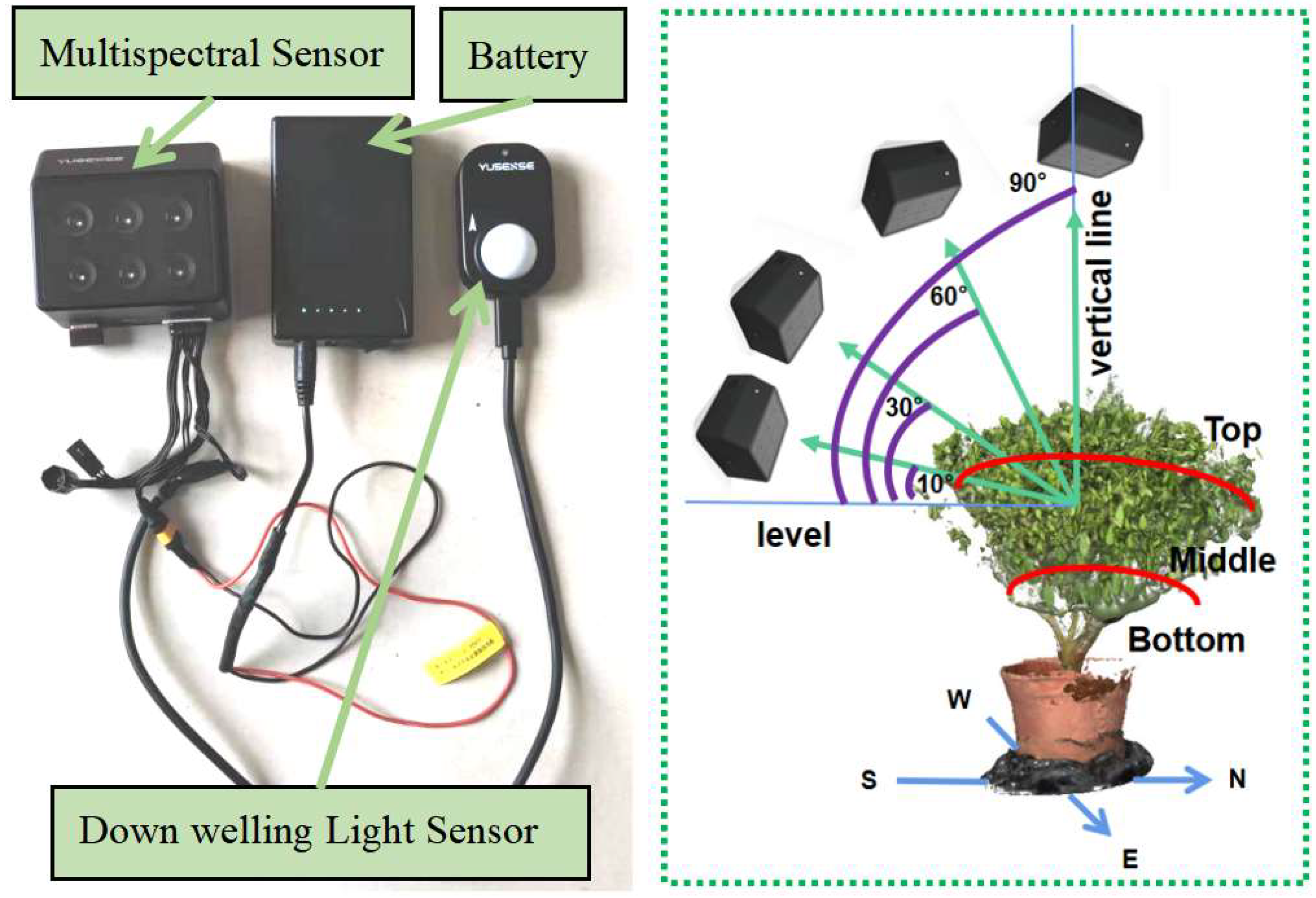
2.2. Data Collection

2.2.1. Spectral Data

The spectral camera used in this experiment was the MS600 V2 (Changguang Yuchen Information Technology and Equipment (Qingdao) Co., Ltd., Qingdao, China). In China, this spectral camera is gradually replacing other imported multispectral cameras with high data quality and an intuitive control system [21].

Table 1. Spectral parameters for the multispectral sensor.

Sensor	CMOS, 1/3″ active pixel: 1.2 MP; global shutter
Angle of Field	HFOV: 49.5°, VFOV: 38.1°; aperture: f/2.2
Spatial Resolution	0.1 cm @ h = 1 m
Image Storage Format	16 bit TIFF, JPEG (reflectivity)
Memory Device	MicroSD card
Operating Temperature Range	−10 °C to 50 °C
Operating Humidity Range	≦85%
Storage Temperature Range	−30 °C to 70 °C
Trigger Mode	Timed trigger, overlap rate trigger, external trigger
Voltage	7–30 V DC
Power Dissipation	7–10 W
Battery Duration	More than 4 h
Size	79 mm × 74 mm × 52 mm
Weight	275 g
Control Software	A web interface accessible by any Wi-Fi device
Attestation	CE, FCC, RoHS
Band Range	Band Number	Band Name	Centre Wavelength (nm)	Bandwidth FWHM (nm)
	1	Blue	450	35
	2	Green	555	25
	3	Red	660	22.5
	4	Red Edge	720	10
	5	Red Edge LP	750	10
	6	Near-infrared	840	30

lists the spectral parameters for the multispectral sensor. For convenience, blue, green, red, red edge, red edge LP, and near-infrared were referred to as B, G, R, ED1, ED2, and NIR, respectively. Figure 3 shows the data acquisition system.

Before acquiring the canopy-scale multispectral image, the calibration plate was first photographed so that the exposure time of the multispectral camera was automatically set to 4 milliseconds. Multispectral images with the sensor line of sight at 10°, 30°, 60°, and 90° from the horizontal direction were sequentially acquired, with the top of the image orientated northward. The angle and orientation were based on corrected sensor data from the locator’s gyroscope (Zhuolin Technology Co., Ltd. (Hefei) Co., Ltd., Hefei, China). In addition, 10 leaves were taken from the 200 g sample collected at each of the four directions at the sampling point to obtain the multispectral image from the front plane view. The acquired multispectral images all contained a whiteboard for correction.

2.2.2. Tea Physiological Data

The top, middle, and bottom of the sampling point were distinguished as shown in Figure 4. The top section sample included the 3rd to 5th leaves from the top of the branch, downwards; the middle section included the 6th to 10th leaves; and the bottom section included the 1st to 5th leaves from the bottom of the branch, upwards. Each leaf was measured thrice from the leaf tip, petiole end, and middle, avoiding the leaf vein. The mean of the value measured by spad-502 plus (Konica Minolta Holdings Co., Ltd., Tokyo, Japan) was considered the SPAD of the leaf. After measurement, the leaves were oven-dried together with other samples and transferred to the laboratory at a third-party professional testing company (Xi’an Guolian Quality Testing Technology Co., Ltd., Xi’an, China) to analyse the total chlorophyll and nitrogen contents. For the convenience of description, the SPAD, total chlorophyll content, and nitrogen content of the assay were collectively referred to as the physiological parameters of the tea.

2.3. Method

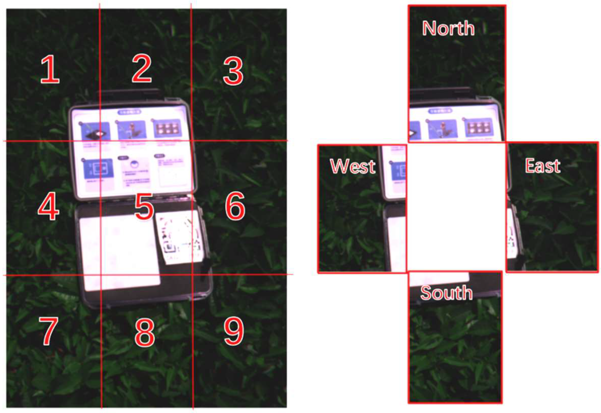
2.3.1. Registration and Fusion

As the sensors of each band of the multispectral camera used in this study were distributed in an array, the acquired images of each channel had a certain deviation in space; however, the camera was not equipped with an automatic registration programme. To facilitate band fusion and spectral information sampling, first, the average digital number (DN) value of the whiteboard in each spectral image was extracted and combined with the reflectivity of each band calibrated using the reference whiteboard. The multispectral DN value image was then converted into a reflectance image in Python 3.6 according to Equation (1):

R_i = DN_i/(DN_w/R_w)

(1)

where R_i is the reflectance image, DN_i is the original DN value image, DN_w is the DN value of the reference whiteboard, and R_w is the calibrated reflectivity of each wavelength band of the reference whiteboard. The Sift algorithm [22] was used to automatically select and match the features of each band image, after which band fusion was performed. Figure 5 shows the effects of before and after registration fusion.

2.3.2. Raster Sampling

To effectively extract partial spectral information from leaves and avoid the influence of backgrounds such as shadows in the image, we proposed a full channel difference vegetation index (FCDVI) for the multispectral images through spectral feature analysis and multiple experiments on leaves and other ground objects in this study. The FCDVI was calculated as follows:

FCDVI = 2 ×(ED1 + NIR) + ED2 + G −8 × (B + R)

(2)

For both leaf- and canopy-scale multispectral images, the FCDVI can significantly enhance the characteristics of tea leaves in multispectral images and increase the contrast with other ground objects for distinguishing tea leaves from the background. Subsequently, the Otsu [23] method was used for image segmentation. Finally, after morphological processing and masking, the pure tea area in the image was obtained. Figure 6 shows the effect of each step during the processing. For the masked image, the average reflectance of each band of the blade was collected as needed to prepare for the subsequent calculation and analysis.

After the canopy image was enhanced by the FCDVI mask, it was automatically batch segmented using Python 3.6. Figure 7 shows the segmentation effect. As the image after the mask was dark and difficult to see, the segmentation effect of the image before the mask is shown here. The image was equally divided into nine small images from left to right and top to bottom. The 2nd, 4th, 6th, and 8th pictures were selected as the four directions of the image. When the top of the image was north, the 2nd, 4th, 6th, and 8th pictures corresponded to the north, west, east, and south directions, respectively. The mean values of each band of the spectral image in these four directions were then extracted separately.

2.3.3. Vegetation Index Construction

We chose to construct indices with better chlorophyll inversion effects than those used in previous studies;

Table 2. Vegetation indices compiled from the literature.

Name	Short Name	Formula	Reference
Normalised difference vegetation index	NDVI	NIR − R/NIR + R	[24]
Normalised difference red edge	NDRE	(NIR − ED)/(NIR + ED)	[25]
Chlorophyll index red edge	CIred edge	(NIR/ED1) − 1	[26]
MERIS terrestrial chlorophyll index	MTCI	(B − G)/(R − ED)	[27]
Modified chlorophyll absorption ratio index	MCARI	(B − G − 0.2(B − R))(B/G)	[28]
Enhanced vegetation index	EVI	2.5(B − G)/(B + 6G − 7.5R + 1)	[29]
Transformed CARI	TCARI	3[(ED1 − R) − 0.2(ED1 − G) ×ED1/R)]	[30]
Modified simple ratio 1	MSR1	(ED2 − B)/(ED1 − B)	[31]
Modified simple ratio 2	MSR2	(NIR/ED1 − 1)/SQRT(NIR/ED1 + 1)	[31]
Chlorophyll index green	CIgreen	(NIR − /G) − 1	[26]
Green normalised difference vegetation index	GNDVI	(NIR − G)/(NIR + G)	[32]
Plant senescence reflectance index	PSRI	(R − G)/ED	[33]
Canopy chlorophyll content index	CCCI	(NIR − ED)/NIR + ED)/(NIR − R)/(NIR + R)	[34]
Nonlinear vegetation index	NLI	(NIR2 − ED)/(NIR2 + ED)	[35]
Triangular greenness index	TGI	G + 0.39×R − 0.61×B	[36]

lists the formulae for calculating them.

2.3.4. Model Training

As the vegetation index dimension was low and the regularisation technology in the selected machine learning algorithm could eliminate redundant problems such as variable collinearity, all the selected vegetation indices and original bands were used as variables for model training. The machine learning algorithms used to train the model included random forest (RF), partial least squares regression (PLS), support vector machine (SVM), and back-propagation neural network (BP). Among them, PLS has often been used to analyse the relationship between multiple dependent and independent variables. It combines the advantages of principal component analysis, normative analysis, and linear regression while effectively obtaining the dominant factor with the strongest explanatory power for the dependent variable. PLS is especially suitable for addressing multicollinearity between variables or when the number of variables is larger than the number of samples [37,38,39]. SVM can provide a more reasonable solution to the above problems than linear methods [40]; it uses a kernel function to map input variables to a high-dimensional feature space [41]. Hence, it can manage high-dimensional input vectors. Recently, SVM has been widely used in spectral analysis and has produced accurate calibration results [42,43,44]. RF is a comprehensive learning algorithm that combines a large number of regression trees that represent a series of conditions or constraints organised in a hierarchy and is applied sequentially from the root to the leaves of the tree. RF starts with multiple bootstrap samples randomly drawn from the original training dataset. Subsequently, a regression tree is applied to each bootstrap sample and a small set of input variables selected from the total set is randomly considered for the binary partition of each tree node [45,46]. The BP neural network, proposed by Rumelhart et al. [47], is a multi-layer feedforward network trained by the error back-propagation algorithm. The training of the BP neural network mainly comprises two processes: forward propagation and error back-propagation. First, the input feature vector is in the forward direction and the predicted class is obtained at the output layer. The predicted category is then compared with the actual corresponding category to obtain the classification error. The parameters of the BP neural network are then trained by the error back-propagation algorithm and the denoising autoencoder parameters of each layer are optimised [48]. In this study, the radial basis function kernel was set in the SVM model training and other parameters were maintained by default. In the training of the RF model, 500 decision trees were set, and other parameters were maintained by default. The BP neural network was set with three hidden layers and a total of 10 neurons. Default settings were used for the other parameters.

2.3.5. Accuracy Evaluation

This study used the leave-one-out cross-validation method for verification, and the final calculated coefficient of determination (R²) and root mean square error (RMSE) to illustrate the advantages and limitations of the model. The closer R² is to 1, the better the model fits; the smaller the RMSE, the smaller the prediction error and the higher the accuracy. All verification methods have been shown to be effective and accurate in machine learning [49]. The calculation method is as follows:

$${\mathrm{R}}^2=1-{\displaystyle {\sum }_{\mathrm{i}=1}^{\mathrm{n}}({\mathrm{x}}_{\mathrm{i}}-{\mathrm{y}}_{\mathrm{i}}}{)}^2/{\displaystyle {\sum }_{\mathrm{i}=1}^{\mathrm{n}}({\mathrm{x}}_{\mathrm{i}}}-\overline{\mathrm{x}}{)}^2$$

(3)

$$\mathrm{RMSE}=\sqrt{{\displaystyle {\sum }_{\mathrm{i}=1}^{\mathrm{n}}{(\mathrm{x}}_{\mathrm{i}}}-{\mathrm{y}}_{\mathrm{i}}{)}^2/\mathrm{n}}$$

(4)

3. Results

3.1. Spatial Differences in the Physiological Parameters of Tea Leaves

The measured SPAD and chlorophyll and nitrogen contents of the tea leaves were grouped vertically (top, middle, and bottom) and horizontally (east, west, south, and north) (Figure 8). Based on the quartiles, the measured physiological data for tea leaves vary considerably in the vertical direction. The SPAD and total chlorophyll content both increase from top to bottom. The nitrogen content of the leaves at the top was the highest, followed by those in the middle. The nitrogen content of those at the bottom was the smallest. This showed that the evaluation of the overall physiological parameters of the tea plant from a single canopy was one-sided. The physiological parameters of the tea leaves must be evaluated individually with a more comprehensive plan. There were also differences in the horizontal direction of the measured physiological data of the tea leaves. In the horizontal direction, the three physiological parameters had similar distributions, i.e., the eastern and southern values were high, whereas the western and northern values were low. This indicated that the physiological parameters of tea were affected by certain factors, resulting in uniform differences in the horizontal direction.

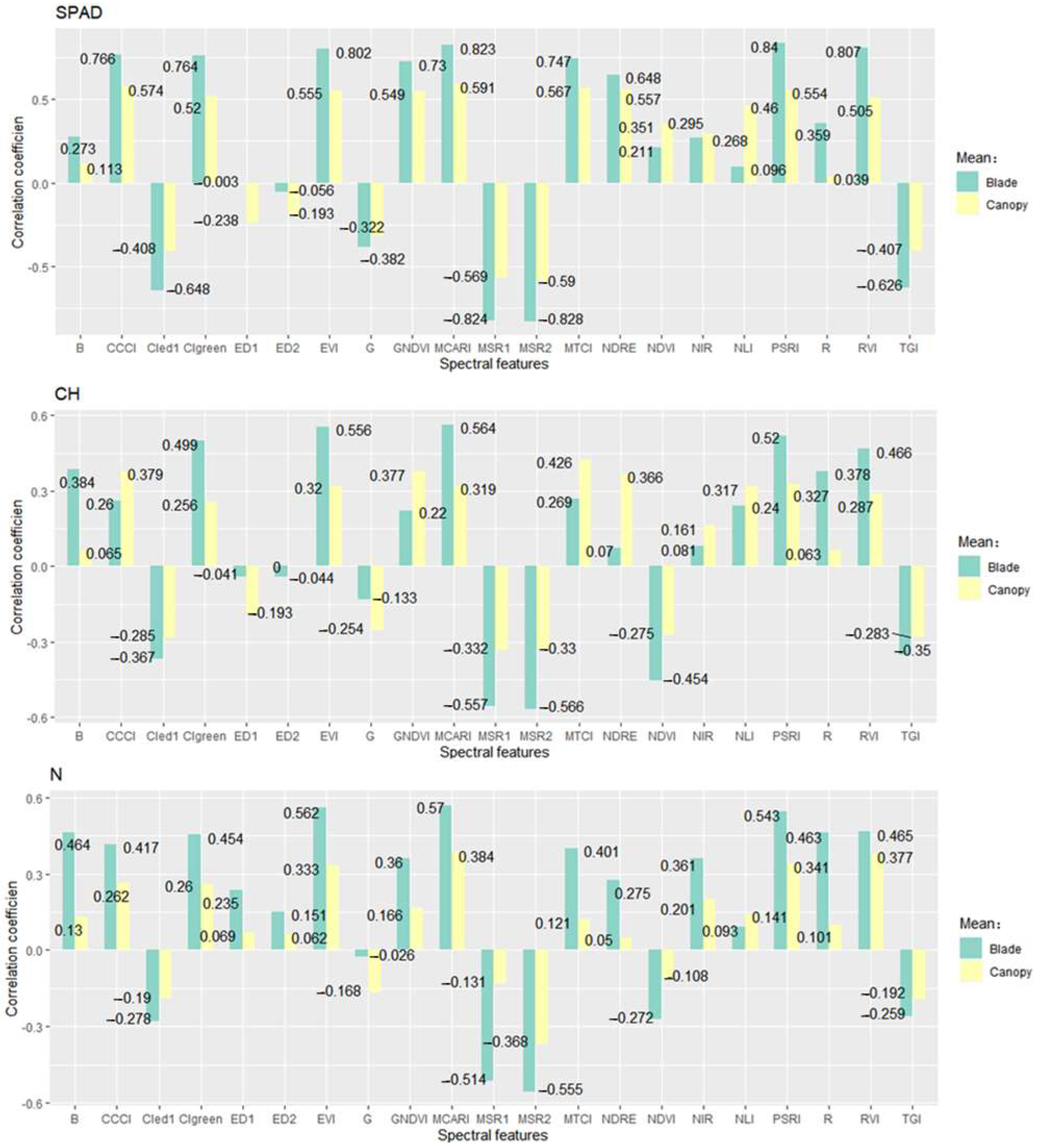
3.2. Correlation Analysis

The indices in Table 2 were calculated from the original multispectral image and the canopy-scale multispectral image enhanced with FCDVI. The correlations between the vegetation index and physiological parameters of the two sets of multispectral images were compared (Figure 9). The vegetation index of the multispectral image with the background objects removed after enhancement of the tea characteristics with the FCDVI showed a better correlation with the physiological parameters of the tea leaves. Both the number of significantly correlated data pairs and the correlation coefficient between most spectral indices and tea physiological parameters increased. This showed that the FCDVI proposed in this study for the MS600 V2 multispectral sensor could substantially enhance the characteristics of tea leaves and assists in removing soil and shadow noise.

Further correlation analysis was carried out between the physiological parameters of the top leaves and the spectral features of the canopy and leaf scales detected perpendicular to the ground. The results are shown in Figure 10. Overall, the correlation between spectral index and SPAD was better than nitrogen content and total chlorophyll content measured in the laboratory. The spectral features of the two scales have obvious similarities. In view of the fact that the leaf spectrum is an important basis for detecting vegetation biochemical parameters, the canopy spectrum is highly similar to it, which confirms that the spectral data in both scales after the FVDVI index removes noise is reliable. In addition, similarly, the correlation between almost all spectral features at the canopy scale and leaf physiological parameters is lower than that at the leaf scale, this shows that the leaf-scale spectral data perpendicular to the ground has a higher signal-to-noise ratio. Although the canopy-scale detection efficiency is higher, it may be difficult to achieve the detection results of the physiological parameters of tea tree leaves in different parts at the leaf scale only by relying on the detection data perpendicular to the ground. Therefore, for the tea tree three-dimensional entity, it is necessary to study the detection of leaf physiological parameters in various parts from multiple detection angles and compare the detection results with the direct detection of leaves.

3.3. Detection Model for Leaf Scale

The spectral data and tea physiological data collected at the leaf and canopy scale were trained by PLS, RF, SVM, and BP neural networks. Figure 11 shows the accuracy of each trained model. First of all, it can be seen intuitively that no matter whether the detection is carried out at the leaf scale or the canopy scale, the best prediction results of the three physiological parameters are SPAD, and the worst are all CH. Moreover, leaf-scale spectral data have better detection accuracy for tea physiological parameters than the canopy scale. This is consistent with the analysis results in Section 3.2, indicating that it is feasible to use multispectral sensors to detect tea physiological parameters at two scales, and, compared with leaf-scale spectral data, there is room for improvement in the detection accuracy at the canopy scale. Secondly, the models trained by the RF and BP algorithms have better performance at the leaf and canopy scales; it shows that the choice of model training algorithms will greatly affect the detection results of various tea physiological parameters, and the selection of model training algorithms will help improve the detection accuracy.

3.4. Optimal Detection Angle for Physiological Parameters of Tea Leaves

The vegetation index calculated from the canopy-scale multispectral images obtained from different shooting angles was used to train the detection model with the physiological parameters of the top, middle, and bottom tea leaves. The RMSE data were normalised with the maximum and minimum values to facilitate easy comparison (Figure 12). Based on the detection results of the three physiological parameters of each part, the detection results at 90° were not the best compared to other angles, while the spectral image acquired at 60° could more comprehensively detect the physiological parameters of the top, middle, and bottom tea leaves. This confirms the previous analysis results that the detection accuracy at the canopy scale has room for improvement, that is, changing the detection angle perpendicular to the ground at the canopy scale can improve the detection accuracy. The detection accuracy of SPAD was still higher than that of CH and N, which is consistent with previous results. In addition, the detection result for the middle leaf was more accurate than that of the top and bottom, which may be related to the selected range of the middle leaves in this study. At last, there existed notable differences among the results of various physiological parameters for the tea leaves from various parts detected at multiple angles, and there was no notable pattern after controlling the variables. In contrast, this showed that the higher-precision non-destructive testing of the tea physiological parameters must consider the detection angle, leaf spatial position, and specific physiological parameters. In other words, we must examine the spatial differences in the tea’s physiological parameters from multiple angles.

4. Discussion

4.1. Multispectral Imagery

The Changguang Yuchen MS600 V2 multispectral sensor has been analysed using various domestic applications [50,51,52]. This has shown that it is stable and reliable. As an improved product of hyperspectral sensors, multispectral sensors are significantly less expensive than both hyperspectral sensors and similar imported equipment [53,54]. These are the most important reasons for choosing the MS600 V2 multispectral camera for this study. MS600 V2 has been integrated with unmanned aerial vehicles (UAVs) for various applications in previous studies, but there are few close-range applications [50,51,55,56]. UAV-integrated applications have more complex data acquisition steps, lower spatial resolution, and increased data processing flows. The ground-portable handheld method proposed in this study can more easily and accurately acquire reliable multispectral data. It should be noted that the registration effect of the multi-view image registration scheme in this study on canopy-scale images with three-dimensional features is not as good as that of leaf-scale two-dimensional feature images, this may be another reason why leaf-scale detection results are better than canopy-scale.

Compared with the original band, the vegetation index constructed by combining multiple bands can highlight some characteristics of vegetation; therefore, it is widely used to monitor physiological and biochemical parameters such as plant biomass, total nitrogen content, and chlorophyll content [57,58]. Therefore, this study selected the vegetation index commonly used for the evaluation of chlorophyll and nitrogen contents, and created the FCDVI index for MS600 V2, which can effectively distinguish the background of green vegetation and soil, and achieved good results. In addition, the vegetation index that had the largest correlation coefficient with the physiological parameters of tea in the correlation analysis was related to R, ED, and NIR, which is consistent with the results of previous studies [59,60,61]. However, the selected vegetation index may still have certain limitations, The discovery or proposal of vegetation indices that have stronger correlations with the physiological parameters of tea can aid in improving the detection accuracy.

The largest difference between the spectral image and non-imaging spectral sensor was that spectral images had the characteristics of wide application and a unified atlas. The spectral images provided spectral information for the target object and obtained spatial information [62,63]. A limited number of previous studies have used the spatial information of spectral images. The division of the top, middle, and bottom physiological parameters and the divisions of the east, south, west, and north spectral images proposed in this study effectively utilised the positional information of spectral images, established a more accurate correspondence between the spectral information and measured target, and improved detection accuracy. The reason for the best detection results of the physiological parameters of tea leaves in the middle may be that the leaves in the middle position defined in this study occupy a larger proportion of the area in the canopy spectral image relative to the top and bottom. On the other hand, the comprehensive result of the detection angle of 60° is the best, which is consistent with the results of a previous study [64]. This may be due to the fact that the spectral images detected at 60° include larger top, middle, and bottom leaf areas and richer spectral reflection information in a balanced manner compared with other detection angles.

4.2. Machine Learning

The PLS, SVM, RF, and BP neural network modelling algorithms used in this study are regression modelling methods that have been widely used in recent remote sensing research and have been shown to be concise and effective [65,66,67,68,69,70]. The training time of the PLS, SVM, RF, and BP neural network algorithms on the same data in Python 3.6 was 7.521, 20.541, 4.521, and 30.214 s, respectively. RF had the best comprehensive prediction results and the highest operating efficiency, which was more conducive to the promotion of efficient and non-destructive testing technology for tea physiological parameters. In the comparison of the various models, PLS was prone to under-fitting, which may be because the relationship between the data was not a simple linear relationship. SVM and BP neural networks were prone to over-fitting and under-fitting, which may be due to the unreasonable parameter settings in the training process, thus requiring more attempts in future studies.

4.3. Physiological Parameters of Tea

The physiological parameters of tea discussed in this study were the measured SPAD and the total chlorophyll and nitrogen contents of the top, middle, and bottom leaves. The SPAD was measured by the Japanese spad-502 plus instrument. This device is designed to quickly obtain a relative value that can characterise the targeted chlorophyll content [71,72]. As the key to plant photosynthesis, the chlorophyll content profoundly affects the efficiency of photosynthesis and the synthesis of important organic compounds in tea leaves. The measurement principle of the SPAD 502 is the same as that of the spectral measurement, i.e., the relative value of chlorophyll is quantitatively calculated using the reflection, transmission, and absorption of light at a specific wavelength band on leaves [73]. Hence, in this study, the SPAD had a strong correlation with the spectral image, and its prediction model has the best accuracy. The correlation between the total chlorophyll content and the spectral image was not as good as that of the SPAD, which may be because chlorophyll a and b should be discussed separately with respect to the total chlorophyll content. To a large extent, the nitrogen content can reflect the content of key organic compounds in tea, Furthermore, detection of the nitrogen content can evaluate the current nutritional status of tea [74]. The prediction model for the nitrogen content had a high prediction accuracy. Related studies have established a relationship between spectral information and nitrogen accumulation [75,76,77] to evaluate the nitrogen nutritional status of tea, which may have better results. In addition, a certain degree of physiological changes in leaves during the period after SPAD was measured on site and before the measurement of chlorophyll and nitrogen content may also cause the correlation between SPAD and spectral images to be better than that of chlorophyll and nitrogen content.

In this study, the physiological parameters of tea differed to varying degrees at different spatial locations. In the east, west, north, and south directions, the values of the tea physiological parameters in the east and south directions were high, whereas the values in the west and north directions were relatively low. This may be attributed to the fact that the study site is located in the northern hemisphere and the testing month was July. For a long period before summer, the sunlight intensity in low-latitude areas is greater than that in high-latitude areas [78], This allowed the southern-facing leaves of the tea plant to be more efficient at photosynthesis, which in turn yielded increased accumulations of nutrients. In addition, in the morning when the sun shines more on the east side of the plant, the environment in which the plant is located has more carbon dioxide accumulation due to night respiration [79]. Compared with the western leaves of the plant in the afternoon, the eastern leaves of the plant have higher photosynthetic efficiency. This study only discussed the differences in the horizontal direction from the measured physiological parameters. Due to space limitations, the effect of using spectral images to detect physiological parameters in various directions was not examined, thus necessitating further research.

5. Conclusions

The tea quality parameters discussed in this study were different in the horizontal and vertical directions due to natural or human factors, especially in the vertical direction. Refining the data to each part of the tea leaf can aid in improving the accuracy of non-destructive detection. There was a significant correlation between the physiological parameters of tea and the spectral index. Therefore, detecting the biophysical and chemical parameters of tea using multispectral technology is feasible. Using the FCDVI proposed in this study, the background noise could be effectively removed and the data quality and correlation were significantly improved. The physiological parameter with the best detection result was SPAD, followed by the nitrogen content and total chlorophyll content. The model trained by the RF algorithm was better than the BP neural network, SVM, and PLS in the detection of tea physiological parameters. The multispectral images at the leaf scale were better than those at the canopy scale in most detecting the physiological parameters of tea leaves, and the change of the detection angle can have a positive effect on the detection effect of the canopy scale closer to the leaf scale. The multispectral images at the canopy scale were better than the top and bottom tea leaves for detecting the physiological parameters of the middle tea leaves. In other words, the precise and accurate correspondence between the spectral information and measured part aided in improving the detection accuracy. The spectral images obtained when the multispectral sensor was at 60° to the horizontal plane could detect the physiological parameters of tea leaves better than when the sensor was at 90°, 30°, and 10°. The model trained using the vegetation index of the spectral image taken at 60° and the RF algorithm had the highest comprehensive accuracy for the detection model of the physiological parameters of the middle tea leaves. The R² of SPAD, chlorophyll, and nitrogen were 0.567, 0.401, and 0.653, respectively, and the RMSEs were 0.365, 0.313, and 0.310, respectively. This can effectively detect the physiological parameters of tea leaves and provide guidance for the refined management of tea gardens.

References

1. Yang, C.S.; Lambert, J.D.; Sang, S. Antioxidative and anti-carcinogenic activities of tea polyphenols. Arch. Toxicol. 2009, 83, 11–21. [Google Scholar] [CrossRef]
2. Han, N.; Mukhtar, H. Green Tea Polyphenols and Metabolites in Prostatectomy. Natl. Health Inst. 2011, 81, 519–533. [Google Scholar]
3. Khan, N.; Mukhtar, H. Tea Polyphenols in Promotion of Human Health. Nutrients 2019, 11, 39. [Google Scholar] [CrossRef] [PubMed]
4. Shao, C.Y.; Zhang, C.Y.; Lv, Z.D. Pre- and post-harvest exposure to stress influence quality-related metabolites in fresh tea leaves. Sci. Hortic. 2021, 281, 109984. [Google Scholar] [CrossRef]
5. Kowalska, J.; Marzec, A.; Domian, E. Influence of Tea Brewing Parameters on the Antioxidant Potential of Infusions and Extracts Depending on the Degree of Processing of the Leaves of Camellia sinensis. Molecules 2021, 26, 4773. [Google Scholar] [CrossRef] [PubMed]
6. Zhang, L.; Zhang, H.D.; Chen, Y.D. Real-time monitoring of optimum timing for harvesting fresh tea leaves based on machine vision. Int. J. Agric. Biol. Eng. 2019, 12, 6–9. [Google Scholar] [CrossRef]
7. Chen, Y.Z.; Wang, F.; Wu, Z.D. Effects of Long-Term Nitrogen Fertilization on the Formation of Metabolites Related to Tea Quality in Subtropical China. Metabolites 2021, 11, 146. [Google Scholar] [CrossRef]
8. Gaudinier, A.; Rodriguez-Medina, J.; Zhang, L.F. Transcriptional regulation of nitrogen-associated metabolism and growth. Nature 2018, 563, 259–264. [Google Scholar] [CrossRef]
9. Raya-Sereno, M.D.; Ortiz-Monasterio, J.I.; Alonso-Ayuso, M. High-Resolution Airborne Hyperspectral Imagery for Assessing Yield, Biomass, Grain N Concentration, and N Output in Spring Wheat. Remote Sens. 2021, 13, 1373. [Google Scholar] [CrossRef]
10. Wu, C.Y.; Wang, L.; Niu, Z. Nondestructive estimation of canopy chlorophyll content using Hyperion and Landsat/TM images. Int. J. Remote Sens. 2010, 31, 2159–2167. [Google Scholar] [CrossRef]
11. Li, W.; Xiang, F.; Su, Y. Gibberellin Increases the Bud Yield and Theanine Accumulation in Camellia sinensis (L.) Kuntze. Molecules 2021, 26, 3290. [Google Scholar] [CrossRef]
12. Yue, C.N.; Wang, Z.H.; Yang, P.X. Review: The effect of light on the key pigment compounds of photosensitive etiolated tea plant. Bot. Stud. 2021, 62, 21. [Google Scholar] [CrossRef]
13. Han, W.Y.; Ma, L.F.; Shi, Y.Z.; Ruan, J.Y.; Kemmitt, S.J. Nitrogen release dynamics and transformation of slow release fertiliser products and their effects on tea yield and quality. J. Sci. Food Agric. 2008, 88, 839–846. [Google Scholar] [CrossRef]
14. Ni, Z.Y.; Lu, Q.F.; Huo, H.Y. Estimation of Chlorophyll Fluorescence at Different Scales: A Review. Sensors 2019, 19, 3000. [Google Scholar] [CrossRef]
15. Saberioon, M.M.; Gholizadeh, A. Novel Approach for Estimating Nitrogen Content in Paddy Fields Using Low Altitude Remote Sensing System. In Proceedings of the 23rd Congress of the International-Society-for-Photogrammetry-and-Remote-Sensing, Prague, Czech Republic, 12–19 July 2016; pp. 1011–2016. [Google Scholar]
16. Mesas-Carrascosa, F.J. UAS-Remote Sensing Methods for Mapping, Monitoring and Modeling Crops. Remote Sens. 2020, 12, 3873. [Google Scholar] [CrossRef]
17. Jia, J.X.; Jiang, C.H.; Li, W. Hyperspectral LiDAR-Based Plant Spectral Profiles Acquisition: Performance Assessment and Results Analysis. Remote Sens. 2021, 13, 2521. [Google Scholar] [CrossRef]
18. Chen, L.Y.; Xu, B.; Zhao, C.J. Application of Multispectral Camera in Monitoring the Quality Parameters of Fresh Tea Leaves. Remote Sens. 2021, 13, 3719. [Google Scholar] [CrossRef]
19. Wilson, D.; Cooper, J.P. Apparent Photosynthesis and Leaf Characters in Relation to Leaf Position and Age, Among Contrasting Lolium Genotypes. New Phytol. 1969, 68, 645. [Google Scholar] [CrossRef]
20. Shaoguan Municipal People’s Government. Available online: https://www.sg.gov.cn/sq/sgjj/lnmj/content/post_1350291.html (accessed on 9 February 2022).
21. Wei, D.D.; Yang, X. Changguang Yuchen: Enriching Informatization with Spectrum. Sci-Tech Innov. Brand. 2020, 4, 62–63. [Google Scholar]
22. Lowe, D.G. Distinctive image features from scale-invariant keypoints. Int. J. Comput. Vis. 2004, 60, 91–110. [Google Scholar] [CrossRef]
23. Otsu, N. A threshold selection method from gray-level histogram. IEEE Trans. Syst. Man Cybern. 1979, 9, 62–66. [Google Scholar] [CrossRef]
24. Rouse, J.W.; Haas, R.H.; Schell, J.A.; Deering, D.W. Monitoring vegetation systems in the great plains with ERTS. In Proceedings of the Third Earth Resources Technology Satellite—1 Symposium, Goddard Space Flight Center, Greenbelt, MD, USA, 10–14 December 1973; pp. 309–317. [Google Scholar]
25. Barnes, E.M.; Clarke, T.R.; Richards, S.E.; Colaizzi, P.D.; Haberland, J.; Kostrzewski, M.; Waller, P.; Choi, C.; Riley, E.; Thompson, T.; et al. Coincident detection of crop water stress, nitrogen status and canopy density using ground based multispectral data. In Proceedings of the Fifth International Conference on Precision Agriculture, Bloomington, MN, USA, 16–19 July 2000; Volume 1619. [Google Scholar]
26. Chen, J.M. Evaluation of Vegetation Indices and a Modified Simple Ratio for Boreal Applications. Can. J. Remote Sens. 1996, 22, 229–242. [Google Scholar] [CrossRef]
27. Dash, J.; Curran, P.J. The MERIS terrestrial chlorophyll index. Int. J. Remote Sens. 2004, 25, 5403–5413. [Google Scholar] [CrossRef]
28. Haboudane, D.; Miller, J.R.; Pattey, E.; Zarco-Tejada, P.J.; Strachan, I.B. Hyperspectral vegetation indices and novel algorithms for predicting green LAI of crop canopies: Modeling and validation in the context of precision agriculture. Remote Sens. Environ. 2004, 90, 337–352. [Google Scholar] [CrossRef]
29. Huete, A.; Didan, J.; Miura, T.; Rodriguez, E.P.; Gao, X.; Ferreira, L.G. Overview of the radiometric and biophysical performance of the MODIS vegetation indices. Remote Sens. Environ. 2002, 83, 195–213. [Google Scholar] [CrossRef]
30. Haboudane, D.; Miller, J.R.; Tremblay, N. Integrated narrow-band vegetation indices for prediction of crop chlorophyll content for application to precision agriculture. Remote Sens. Environ. 2002, 81, 416–426. [Google Scholar] [CrossRef]
31. Xie, Q.Y.; Huang, W.J.; Zhang, B.; Chen, P.F.; Song, X.Y.; Pascucci, S.; Pignatti, S.; Laneve, G.; Dong, Y.Y. Estimating Winter Wheat Leaf Area Index From Ground and Hyperspectral Observations Using Vegetation Indices. IEEE J. Sel. Top. Appl. Earth Observ. Remote Sens. 2016, 9, 771–780. [Google Scholar] [CrossRef]
32. Gitelson, A.A.; Kaufman, Y.J.; Merzlyak, M.N. Use of a green channel in remote sensing of global vegetation from EOS-MODIS. Remote Sens. Environ. 1996, 58, 289–298. [Google Scholar] [CrossRef]
33. Merzlyak, M.N.; Gitelson, A.A.; Chivkunova, O.B.; Rakitin, V.Y. Non-destructive optical detection of pigment changes during leaf senescence and fruit ripening. Physiol. Plant. 1999, 106, 135–141. [Google Scholar] [CrossRef]
34. El-Shikha, D.M.; Barnes, E.M.; Clarke, T.R.; Hunsaker, D.J.; Haberland, J.A.; Pinter, P.J., Jr.; Waller, P.M.; Thompson, T.L. Remote sensing of cotton nitrogen status using the canopy chlorophyll content index (CCCI). Trans. ASABE 2008, 51, 73–82. [Google Scholar] [CrossRef]
35. Goel, N.S.; Qin, W. Influences of canopy architecture on relationships between various vegetation indices and LAI and Fpar: A computer simulation. Int. J. Remote Sens. 1994, 10, 309–347. [Google Scholar] [CrossRef]
36. Hunt, E.R.; Doraiswamy, P.C.; McMurtrey, J.E.; Daughtry, C.S.T.; Perry, E.M.; Akhmedov, B. A visible band index for remote sensing leaf chlorophyll content at the canopy scale. Int. J. Appl. Earth Obs. Geoinf. 2013, 21, 103–112. [Google Scholar] [CrossRef] [Green Version]
37. Wold, S.; Ruhe, A.; Wold, H.; Dunn, W.J. The collinearity problem in linear regression. The partial least squares (PLS) approach to generalized inverses. SIAM J. Sci. Stat. Comput. 1984, 5, 735–743. [Google Scholar] [CrossRef]
38. Abdi, H. Partial least square regression (PLS Regression). In Encyclopedia of Social Science Research Methods; SAGE: Thousand Oaks, CA, USA, 2003; pp. 792–795. [Google Scholar]
39. Peng, X.; Shi, T.; Song, A.; Chen, Y.; Gao, W. Estimating soil organic carbon using VIS/NIR spectroscopy with SVMR and SPA methods. Remote Sens. 2014, 6, 2699–2717. [Google Scholar] [CrossRef]
40. Walczak, B.; Massart, D.L. The radial basis functions—Partial least squares approach as a flexible non-linear regression technique. Anal. Chim. Acta. 1996, 331, 177–185. [Google Scholar] [CrossRef]
41. Viscarra, R.R.; Behrens, T. Using data mining to model and interpret soil diffuse reflectance spectra. Geoderma 2010, 158, 46–54. [Google Scholar]
42. Zhu, D.; Ji, B.; Meng, C.; Shi, B.; Tu, Z.; Qing, Z. The performance of ν-support vector regression on determination of soluble solids content of apple by acousto-optic tunable filter near-infrared spectroscopy. Anal. Chim. Acta 2007, 598, 227–234. [Google Scholar] [CrossRef]
43. Balabin, R.M.; Safieva, R.Z.; Lomakina, E.I. Comparison of linear and nonlinear calibration models based on near infrared (NIR) spectroscopy data for gasoline properties prediction. Chemom. Intell. Lab. Syst. 2007, 88, 183–188. [Google Scholar] [CrossRef]
44. Li, Y.; Shao, X.; Cai, W. A consensus least squares support vector regression (LS-SVR) for analysis of near-infrared spectra of plant samples. Talanta 2007, 72, 217–222. [Google Scholar] [CrossRef]
45. Breiman, L. Random forests. Mach. Learn. 2001, 45, 5–32. [Google Scholar] [CrossRef]
46. Rodriguez-Galiano, V.; Mendes, M.P.; Garcia-Soldado, M.J.; Chica-Olmo, M.; Ribeiro, L. Predictive modeling of groundwater nitrate pollution using random forest and multisource variables related to intrinsic and specific vulnerability: A case study in an agricultural setting (southern Spain). Sci. Total Environ. 2014, 476, 189–206. [Google Scholar] [CrossRef] [PubMed]
47. Rumelhart, D.E.; Hinton, G.E.; Williams, R.J. Learning representations by back-propagation errors. Nature 1986, 323, 533–536. [Google Scholar] [CrossRef]
48. Liang, P.; Shi, W.Z.; Zhang, X.K. Remote Sensing Image Classification Based on Stacked Denoising Autoencoder. Remote Sens. 2018, 10, 16. [Google Scholar] [CrossRef] [Green Version]
49. Kohavi, R. A study of cross-validation and bootstrap for accuracy estimation and model selection. In Proceedings of the International Joint Conference on Artificial Intelligence, Montreal, QC, Canada, 1 January 1995; pp. 1137–1143. [Google Scholar]
50. Zhang, Y.F.; Zhao, F.; Kou, W.L. Application of UAV in Forest Disaster Monitoring. World For. Res. 2020, 33, 2. [Google Scholar]
51. Zhu, W.X.; Sun, Z.G.; Li, B.B. Soil spatial heterogeneity analysis and crop spectral index response stress diagnosis in coastal saline-alkali land based on UAV remote sensing. J. Geo-Inf. Sci. 2021, 23, 3. [Google Scholar]
52. Liu, C.; Xue, Y. Analysis on performance evaluation method of airborne low-altitude multispectral sensor. Geotech. Investig. Surv. 2021, 11, 201–231. [Google Scholar]
53. Qin, J.W.; Chao, K.L.; Kim, M.S.; Lu, R.F.; Burks, T.F. Hyperspectral andmultispectral imaging for evaluating food safety and quality. J. Food Eng. 2013, 118, 157–171. [Google Scholar] [CrossRef]
54. Feng, C.H.; Makino, Y.; Oshita, S.; Martín, J.F.G. Hyperspectral imaging and multispectral imaging as the novel techniques for detecting defects in raw and processed meat products: Current state-of-the-art research advances. Food Control 2018, 84, 165–176. [Google Scholar] [CrossRef]
55. Zhang, F.Y.; Hu, Y.M.; Xie, Y.K. Integrated design of mobile laboratory for quality monitoring of cultivated land in the sky and land. J. Agric. Res. Environ. 2021, 38, 1029–1038. [Google Scholar]
56. Zhao, J.; Yan, C.Y.; Yang, D.J. Extraction of corn lodging information after typhoon based on UAV multispectral remote sensing. Trans. Chin. Soc. Agric. Eng. 2021, 37, 56–64. [Google Scholar]
57. Xue, J.R.; Su, B.F. Significant remote sensing vegetation indices: A review of developments and applications. J. Sens. 2017, 2017, 1353691. [Google Scholar] [CrossRef]
58. Kamble, B.; Kilic, A.; Hubbard, K. Estimating crop coefficients using remote sensing-based vegetation index. Remote Sens. 2012, 4, 1588–1602. [Google Scholar] [CrossRef]
59. Su, J.Y.; Liu, C.C.; Hu, X.P.; Xu, X.M.; Guo, L.; Chen, W.H. Spatio-temporal monitoring of wheat yellow rust using UAV multispectral imagery. Comput. Electron. Agric. 2019, 167, 105035. [Google Scholar] [CrossRef]
60. Belgiu, M.; Dragut, L. Random forest in remote sensing: A review of applications and future directions. ISPRS—J. Photogramm. Remote Sens. 2016, 114, 24–31. [Google Scholar] [CrossRef]
61. Kawamura, K.; Asai, H.; Yasuda, T.; Soisouvanh, P.; Phongchanmixay, S. Discriminating crops/weeds in an upland rice field from UAV images with the SLIC-RF algorithm. Plant Prod. Sci. 2021, 24, 198–215. [Google Scholar] [CrossRef]
62. Zhang, L.P.; Huang, X.; Huang, B.; Li, P.X. A pixel shape index coupled with spectral information for classification of high spatial resolution remotely sensed imagery. IEEE Trans. Geosci. Remote Sens. 2006, 44, 2950–2961. [Google Scholar] [CrossRef]
63. Pla, F.; Gracia, G.; Garcia-Sevilla, P.; Mirmehdi, M.; Xie, X.H. Multi-spectral texture characterisation for remote sensing image segmentation. In Proceedings of the Lecture Notes in Computer Science, Pattern Recognition and Image Analysis, IbPRIA 2009, Povoa de Varzim, Portugal, 10–12 June 2009; Springer: Berlin/Heidelberg, Germany, 2009; p. 257. [Google Scholar]
64. Guo, J.M.; Gao, Y.; Li, S.T. Estimation model of winter wheat leaf moisture content based on multi-angle hyperspectral remote sensing. J. Anhui Agric. Univ. 2019, 46, 124–132. [Google Scholar]
65. Camps-Valls, G.; Bruzzone, L.; Rojo-Alvarez, J.L.; Melgani, F. Robust support vector regression for biophysical variable estimation from remotely sensed images. IEEE Geosci. Remote Sens. Lett. 2006, 3, 339–343. [Google Scholar] [CrossRef]
66. Lary, D.J.; Alavi, A.H.; Gandomi, A.H.; Walker, A.L. Machine learning in geosciences and remote sensing. Geosci. Front. 2016, 7, 3–10. [Google Scholar] [CrossRef] [Green Version]
67. Maimaitijiang, M.; Sagan, V.; Sidike, P. Comparing support vector machines to PLS for spectral regression applications. Remote Sens. 2020, 12, 1357. [Google Scholar] [CrossRef]
68. Sun, J.; Lu, X.Z.; Mao, H.P.; Wu, X.H.; Gao, H.Y. Quantitative Determination of Rice Moisture Based on Hyperspectral Imaging Technology and BCC-LS-SVR Algorithm. J. Food Process Eng. 2017, 40, e12446. [Google Scholar] [CrossRef]
69. Bischof, H.; Schneider, W.; Pinz, A.J. Multispectral classification of Landsat-images using neural networks. IEEE Trans. Geosci. Remote Sens. 1992, 30, 482–490. [Google Scholar] [CrossRef]
70. Zhang, J.; Fang, S.; Liu, H.H. Machine Learning Approach for Estimation of Crop Yield Combining Use of Optical and Microwave Remote Sensing Data. J. Geo-Inf. Sci. 2021, 23, 1082–1091. [Google Scholar]
71. Shibaeva, T.G.; Mamaev, A.V.; Sherudilo, E.G. Evaluation of a SPAD-502 Plus Chlorophyll Meter to Estimate Chlorophyll Content in Leaves with Interveinal Chlorosis. Russ. J. Plant Physiol. 2020, 67, 690–696. [Google Scholar] [CrossRef]
72. Chen, C.; Zhang, Y.C. The Difference Between Stomatal Density and Chlorophyll Content of Different Potato Varieties. Chin. Agric. Sci. Bull. 2013, 29, 83–87. [Google Scholar]
73. Khorramnia, K.; Khot, L.R.; Shariff, A.R. Oil Palm Leaf Nutrient Estimation by Optical Sensing Techniques. Trans. ASABE 2014, 57, 1267–1277. [Google Scholar]
74. Verkroost, A.W.; Wassen, M.J. A simple model for nitrogen-limited plant growth and nitrogen allocation. Ann. Bot. 2005, 95, 871–876. [Google Scholar] [CrossRef]
75. Xu, K.; Zhang, J.C.; Li, H.M. Spectrum- and RGB-D-Based Image Fusion for the Prediction of Nitrogen Accumulation in Wheat. Remote Sens. 2021, 12, 4040. [Google Scholar] [CrossRef]
76. Tan, C.W.; Du, Y.; Zhou, J. Analysis of Different Hyperspectral Variables for Diagnosing Leaf Nitrogen Accumulation in Wheat. Front. Plant Sci. 2018, 9, 674. [Google Scholar] [CrossRef]
77. Zheng, H.B.; Cheng, T.; Li, D. Evaluation of RGB, Color-Infrared and Multispectral Images Acquired from Unmanned Aerial Systems for the Estimation of Nitrogen Accumulation in Rice. Remote Sens. 2018, 10, 824. [Google Scholar] [CrossRef]
78. Wilhelm, S.; Stober, G.; Matthias, V. Connection between the length of day and wind measurements in the mesosphere and lower thermosphere at mid- and high latitudes. Ann. Geophys. 2019, 37, 1–14. [Google Scholar] [CrossRef]
79. Ainsworth, E.A.; Long, S.P. What have we learned from 15 years of free-air CO2 enrichment (FACE)? A meta-analytic review of the responses of photosynthesis, canopy. New Phytol. 2005, 165, 351–371. [Google Scholar] [CrossRef]
Figure 1. Geographical location of the study area.
Remotesensing 15 00935 g001
Figure 2. Experimental steps.
Remotesensing 15 00935 g002
Figure 3. Data acquisition system.
Remotesensing 15 00935 g003
Figure 4. Schematic diagram of the sampling locations.
Remotesensing 15 00935 g004
Figure 5. Comparison before and after registration. (a) Before leaf-scale multispectral image registration and fusion; (b) after leaf-scale multispectral image registration and fusion; (c) canopy-scale multispectral image before registration and fusion; and (d) canopy-scale multispectral image after registration and fusion.
Remotesensing 15 00935 g005
Figure 6. Images corresponding to the different steps of the background removal process. (a) Original multispectral image pre-processed at leaf scale; (b) multispectral image enhanced with the full channel difference vegetation index; (c) image after binarisation with Otsu; (d) image with binarisation of the multispectral image after masking the original multispectral image; and (eh) canopy-scale spectral images processed in the same order as (ad), respectively.
Remotesensing 15 00935 g006
Figure 7. Canopy-scale image segmentation by orientation.
Remotesensing 15 00935 g007
Figure 8. Spatial differences in the physiological parameters of tea. Dots represent outliers, the upper and lower ends of the vertical line represent the maximum and minimum values, respectively, the top and bottom lines of the box represent the upper and lower quartiles, respectively, and the horizontal line in the box represents the median. SPAD, the value measured with the spad-502 plus instrument; CH, total chlorophyll content; and N, total nitrogen content.
Remotesensing 15 00935 g008
Figure 9. Correlation between vegetation index and tea physiological parameters calculated from multispectral images before and after full channel difference vegetation index enhancement. The blank sections indicate failed significance tests. NDVI, normalised difference vegetation index; NDRE, normalised difference red edge; CIed1, chlorophyll index red edge; MTCI, MERIS terrestrial chlorophyll index; MCARI, modified chlorophyll absorption ratio index; EVI, enhanced vegetation index; TCARI, transformed CARI; MSR1, modified simple ratio 1; MSR2, modified simple ratio 2; CIgreen, chlorophyll index green; GNDVI, green normalised difference vegetation index; PSRI, plant senescence reflectance index; CCCI, canopy chlorophyll content index; NLI, nonlinear vegetation index; TGI, triangular greenness index; SPAD, value measured using the spad-502 plus instrument; CH, total chlorophyll content; and N, total nitrogen content.
Remotesensing 15 00935 g009
Figure 10. Correlation coefficients of leaf physiological parameters at the top with vertical ground-probe spectral features. Blade represents the vegetation index calculated from the leaf-scale multispectral images. Canopy represents the vegetation index calculated from the canopy-scale multi-hyperspectral images. SPAD, the value measured with the spad-502 plus instrument; CH, total chlorophyll content; and N, total nitrogen content.
Remotesensing 15 00935 g010
Figure 11. Accuracy comparison of various algorithm models at leaf and canopy scale. SPAD represents the value measured with the spad-502 plus instrument, CH represents the total chl, N represents the nitrogen.
Remotesensing 15 00935 g011
Figure 12. Comparison of the accuracy of detecting the physiological parameters for tea leaves at different positions and angles. SPAD represents the value measured with the spad-502 plus instrument, CH represents the total chlorophyll content, N represents the total nitrogen content, RMSE represents the root mean square error, and R2 represents the coefficient of determination.
Remotesensing 15 00935 g012