

Data-Independent Phase-Only Beamforming of FDA-MIMO Radar for Swarm Interference Suppression


Abstract
1. Introduction
- (1)
- We propose two data-independent phase-only beamforming methods for FDA-MIMO to suppress the swarm interference.
- (2)
- Our proposed algorithms can achieve interference suppression by only tuning the phase of the weight vector, which efficiently reduces the hardware cost of the FDA-MIMO radar.
- (3)
- Our proposed dual-phase shifter receiver for FDA-MIMO can convert other complex weight vector beamforming methods to phase-only beamforming.
- (4)
- The proposed method can obtain excellent output SINR with a small number of snapshots.
2. Signal Model of FDA-MIMO Radar
3. Analysis of Adaptive Beamforming in Interference Suppression
4. Data-Independent Phase-Only Beamforming
4.1. Constant Modulus Constraint
| Algorithm 1: Proposed CMC Algorithm. |
|
4.2. Constant Modulus Decomposition
| Algorithm 2: Proposed CMD Algorithm. |
|
5. Simulation Results
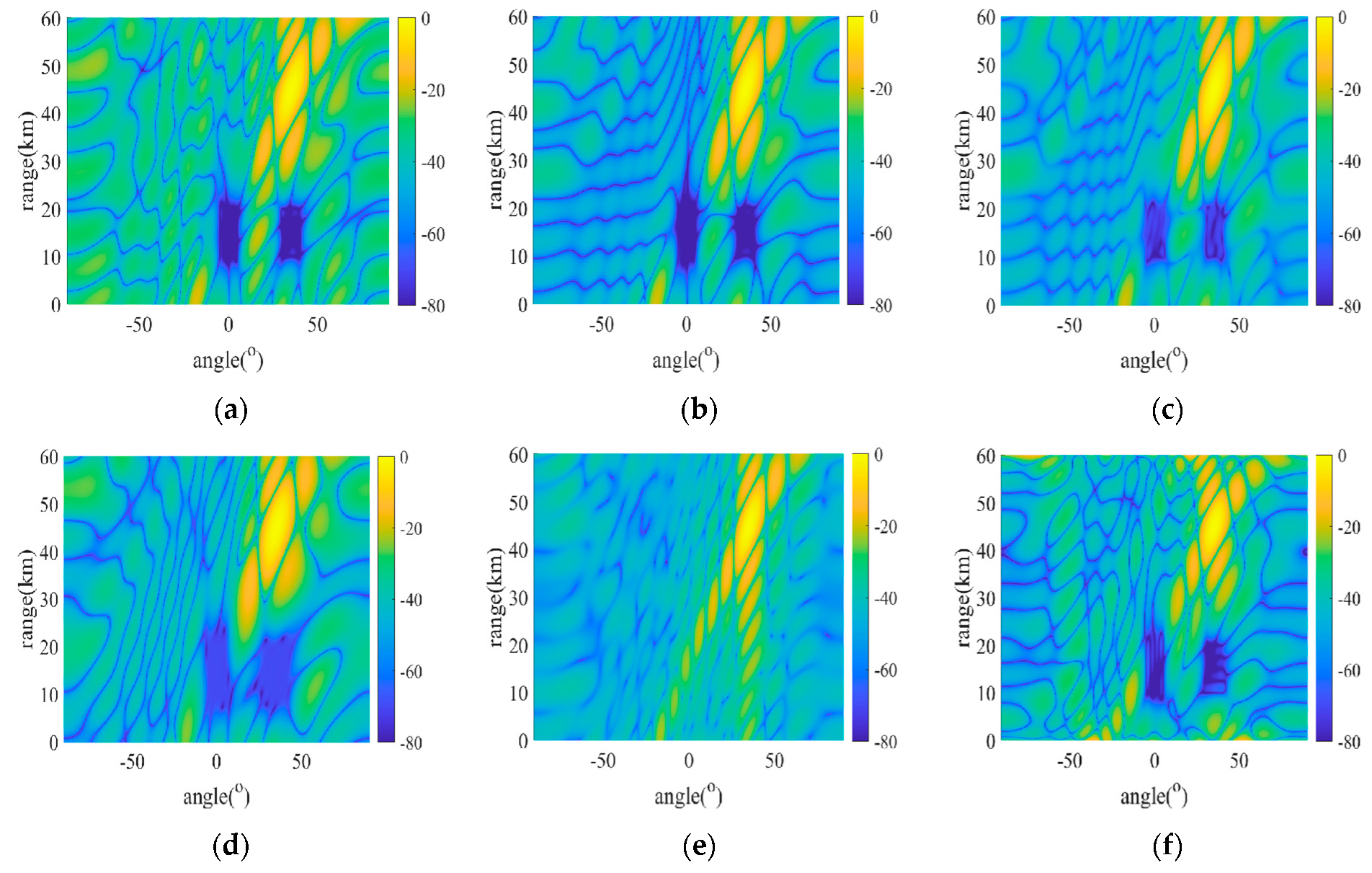
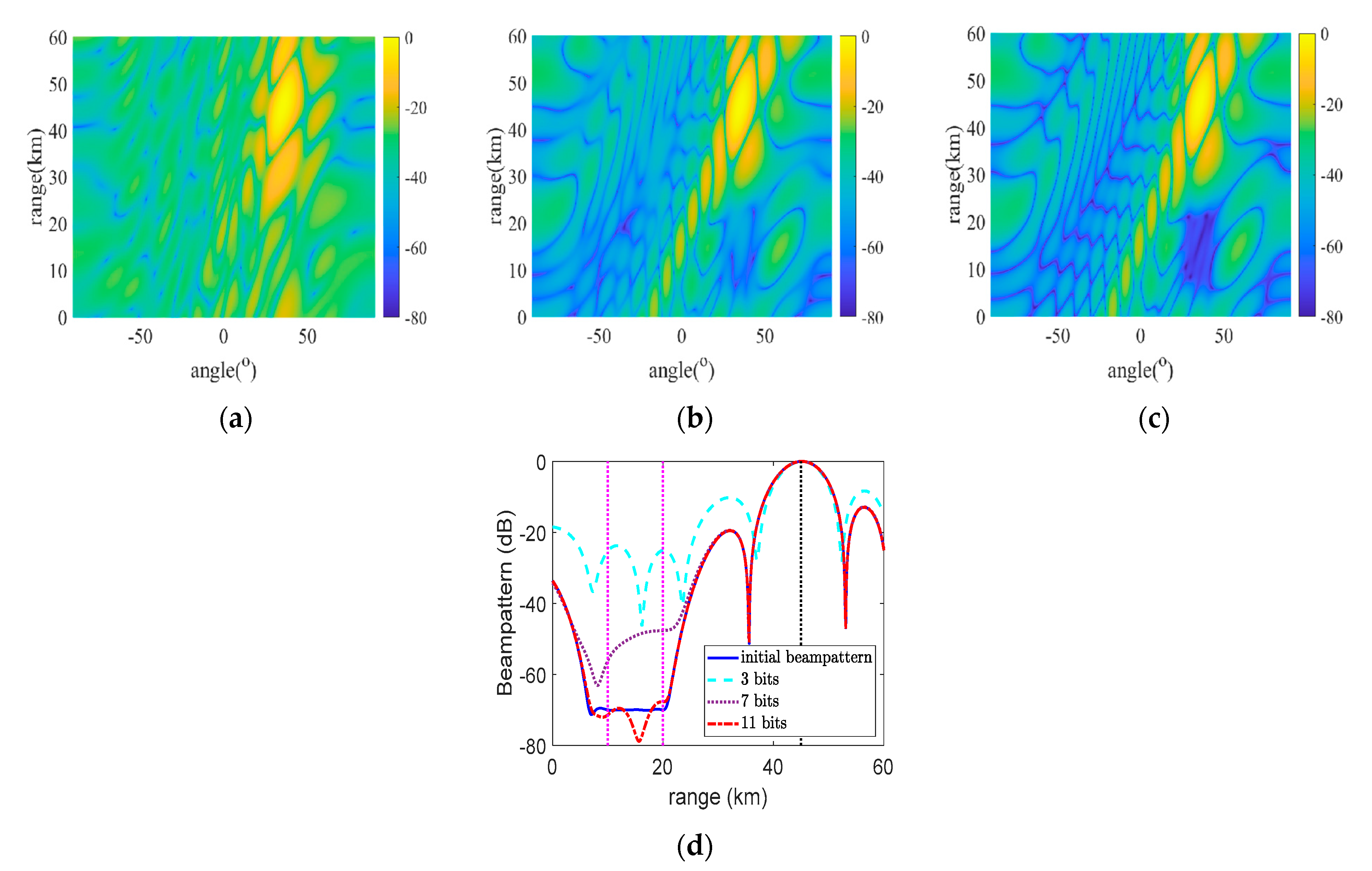
5.1. Beampattern Comparison for Different Algorithms
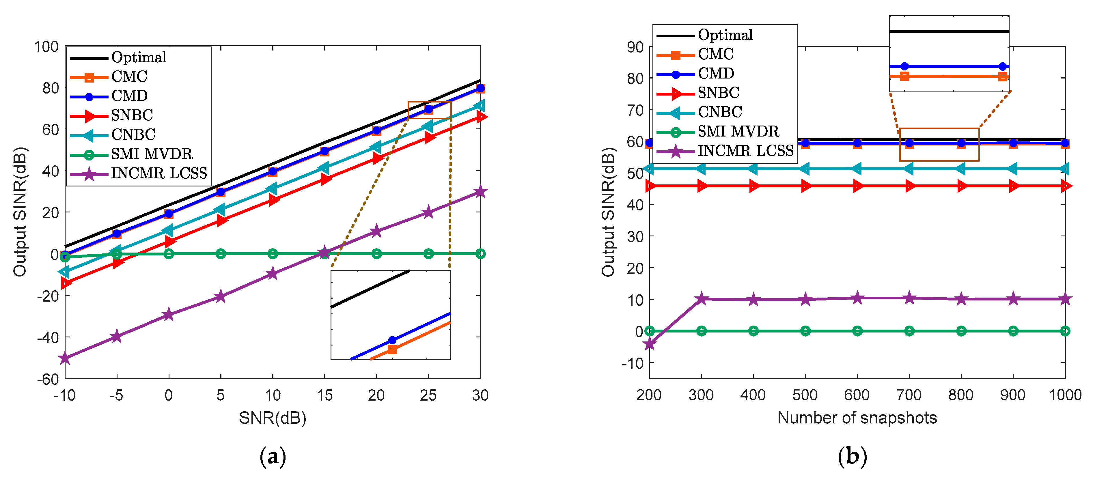
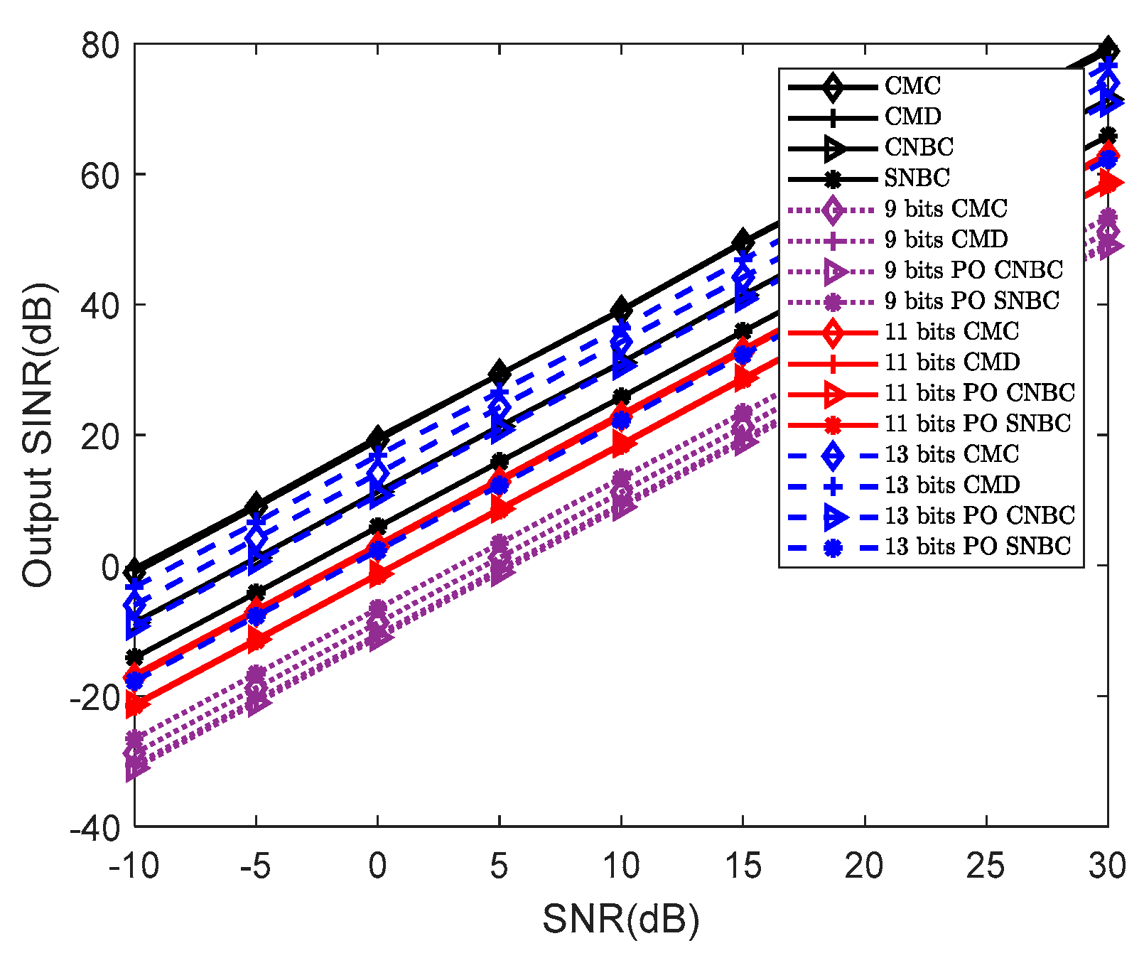
5.2. Comparison of the Output SINR
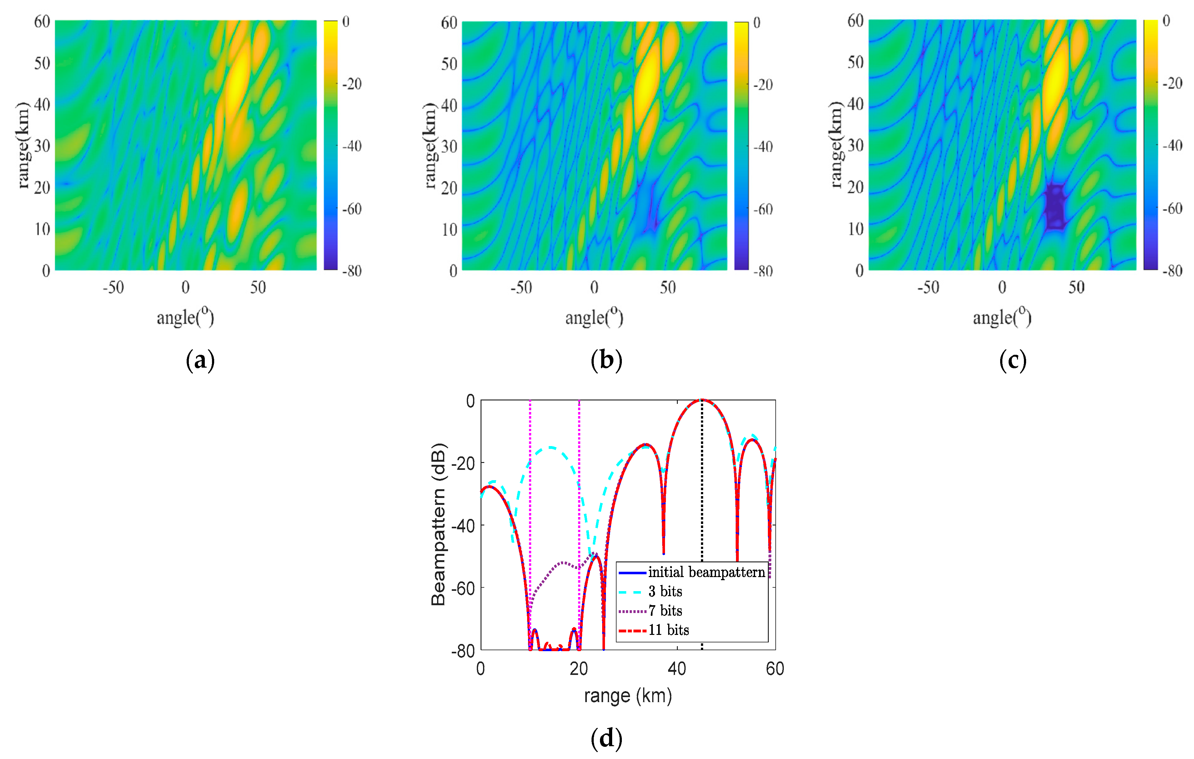
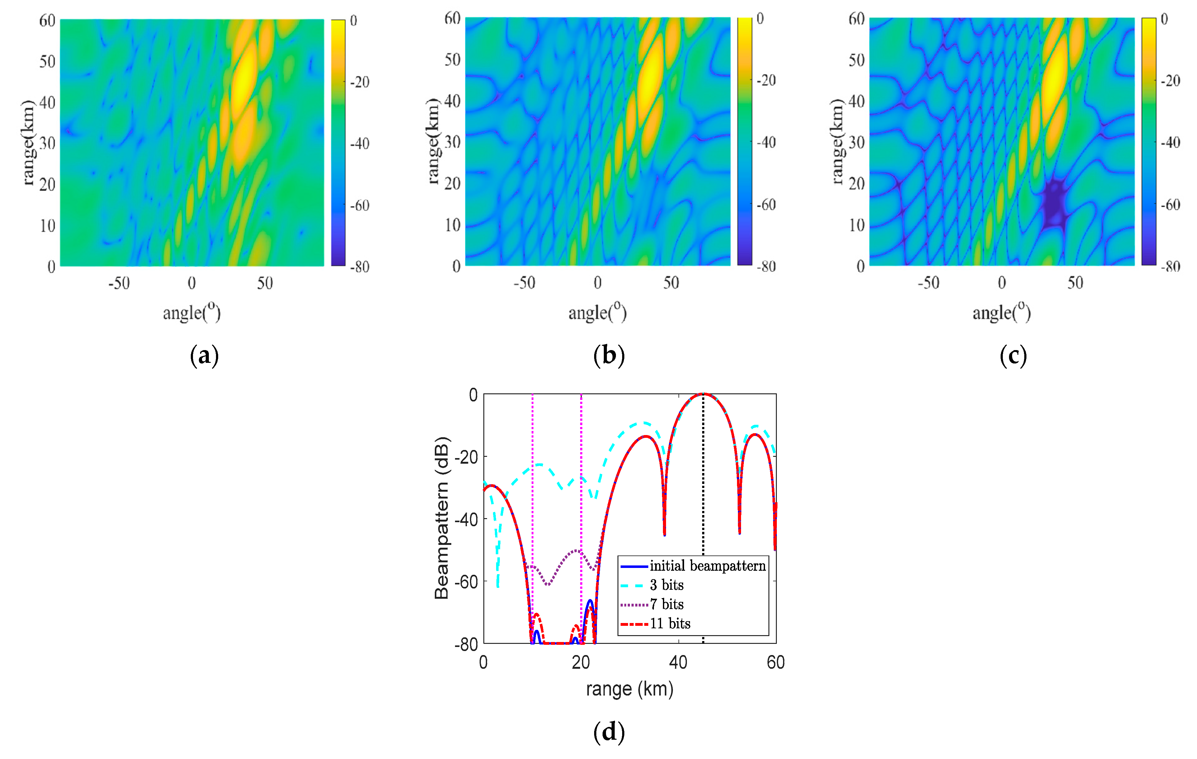
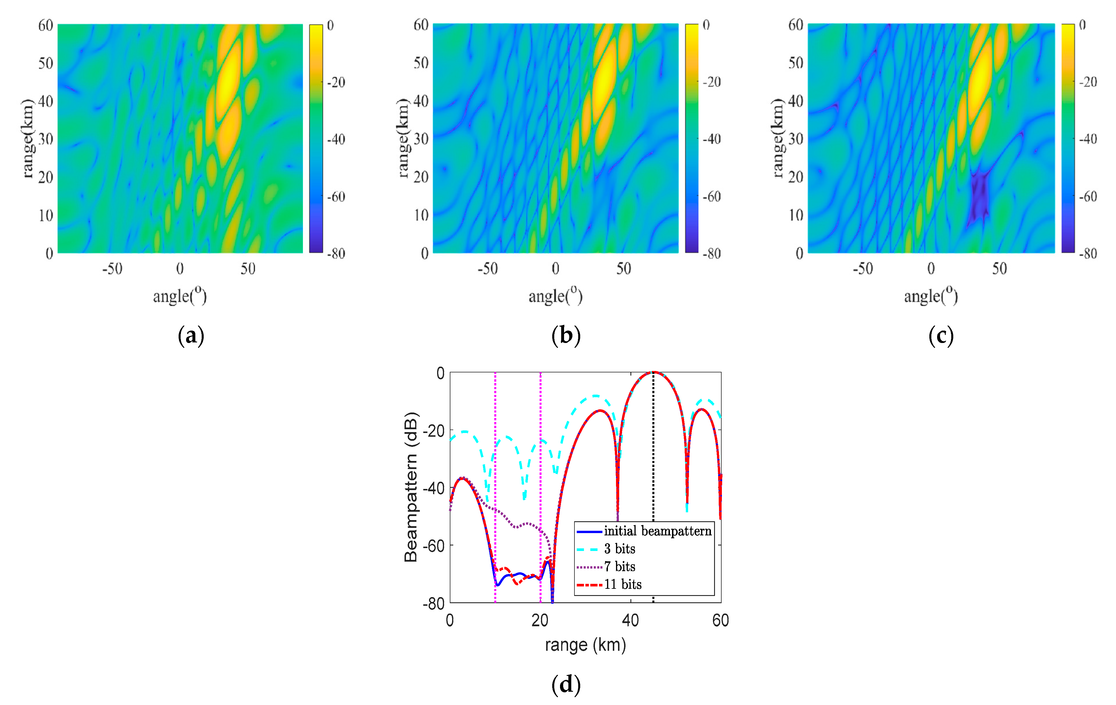
5.3. Beampattern on the Different Quantization Bits
5.4. Output SINR on the Different Quantization Bits
6. Conclusions
Author Contributions
Funding
Data Availability Statement
Conflicts of Interest
Appendix A
Appendix B
- (1)
- When , there is , and the above formula is obviously established.
- (2)
- When , there is , , and then .
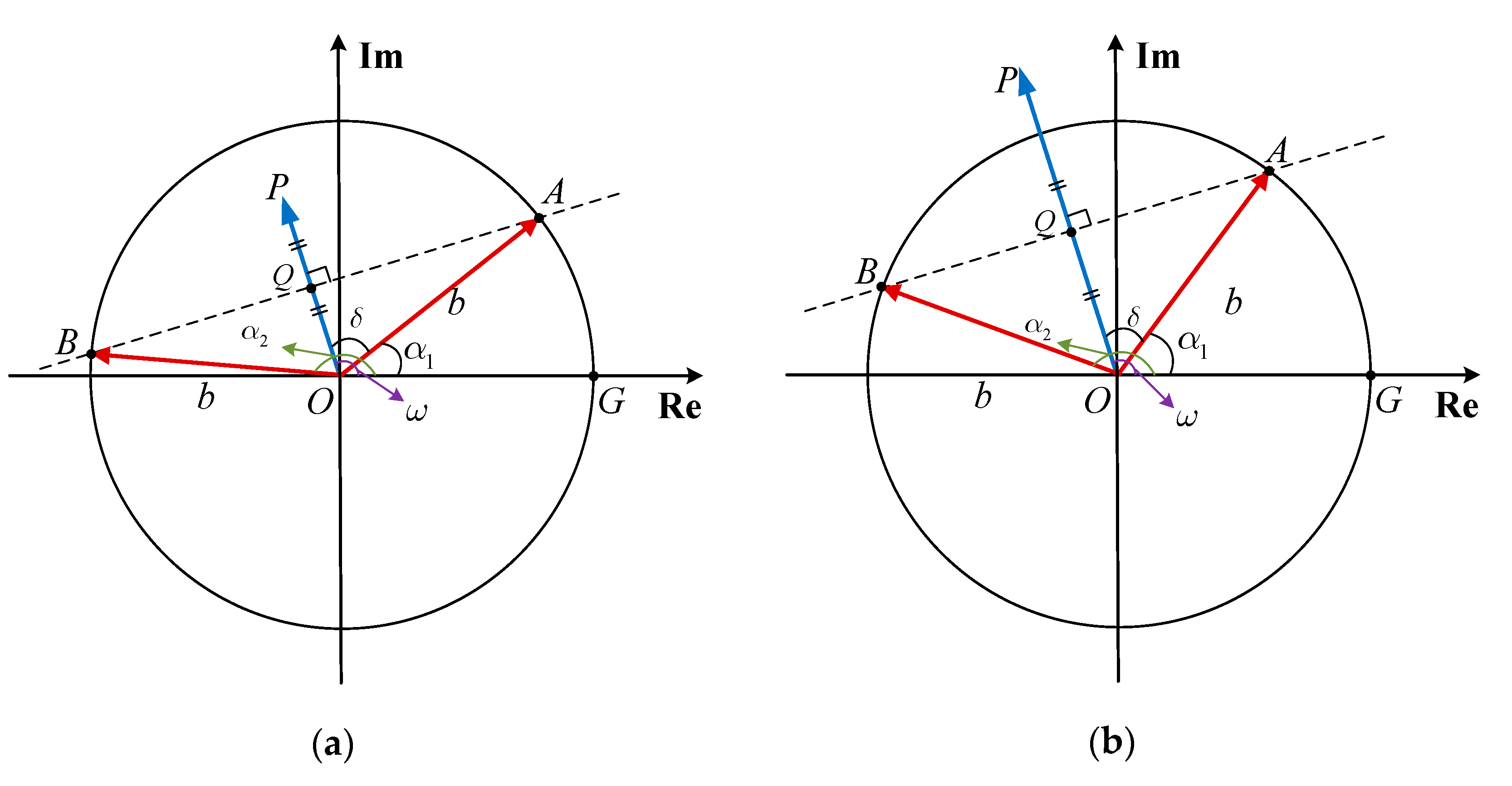
- (3)
- Consider the common case that , we plot in the complex plane, as shown in Figure A1, where denotes the complex and . After that, find the midpoint of the such that . We make a vertical line of through point Q and intersect the circle of radius at points A and B, i.e., . Therefore, we obviously find .

References
- Zheng, Z.; Yang, T.; Wang, H.C. Robust Adaptive Beamforming via Simplified Interference Power Estimation. IEEE Trans. Aerosp. Electron. Syst. 2019, 55, 3139–3152. [Google Scholar] [CrossRef]
- Zhang, X.; He, Z.; Liao, B.; Zhang, X.; Yang, Y. Pattern Synthesis via Oblique Projection-Based Multipoint Array Response Control. IEEE Trans. Antennas Propag. 2019, 67, 4602–4616. [Google Scholar] [CrossRef]
- Ge, Q.; Zhang, Y.; Wang, Y.; Zhang, D. Multi-Constraint Adaptive Beamforming in the Presence of the Desired Signal. IEEE Commun. Lett. 2020, 24, 2594–2598. [Google Scholar] [CrossRef]
- Li, Z.; Zhang, Y.; Ge, Q.; Guo, Y. Middle Subarray Interference Covariance Matrix Reconstruction Approach for Robust Adaptive Beamforming with Mutual Coupling. IEEE Commun. Lett. 2019, 23, 664–667. [Google Scholar] [CrossRef]
- Zhang, X.; Wang, X.; So, H.C. Linear Arbitrary Array Pattern Synthesis with Shape Constraints and Excitation Range Control. IEEE Antennas Wirel. Propag. Lett. 2021, 20, 1018–1022. [Google Scholar] [CrossRef]
- Wang, X.; Amin, M.; Cao, X. Analysis and Design of Optimum Sparse Array Configurations for Adaptive Beamforming. IEEE Trans. Signal Process. 2018, 66, 340–351. [Google Scholar] [CrossRef]
- Zhou, X.; Wen, X.; Wang, Z. Swarm of micro flying robots in the wild. Sci. Robot 2022, 7, eabm5954. [Google Scholar] [CrossRef]
- Soria, E. Swarms of flying robots in unknown environments. Sci. Robot 2022, 7, eabq2215. [Google Scholar] [CrossRef]
- Amar, A.; Doron, M. A linearly constrained minimum variance beamformer with a pre-specified suppression level over a pre-defined broad null sector. Signal Process. 2015, 109, 165–171. [Google Scholar] [CrossRef]
- Liu, J.; Liu, W.; Liu, H.; Chen, B.; Xia, X.; Dai, F. Average SINR Calculation of a Persymmetric Sample Matrix Inversion Beamformer. IEEE Trans. Signal Process. 2016, 64, 2135–2145. [Google Scholar] [CrossRef]
- Gu, Y.; Leshem, A. Robust Adaptive Beamforming Based on Interference Covariance Matrix Reconstruction and Steering Vector Estimation. IEEE Trans. Signal Process. 2012, 60, 3881–3885. [Google Scholar]
- Gu, Y.; Goodman, N.; Hong, S.; Li, Y. Robust adaptive beamforming based on interference covariance matrix sparse reconstruction. Signal Process. 2014, 96, 375–381. [Google Scholar] [CrossRef]
- Zhang, X.; He, Z.; Liao, B.; Zhang, X.; Cheng, Z.; Lu, Y. A2RC: An Accurate Array Response Control Algorithm for Pattern Synthesis. IEEE Trans. Signal Process. 2017, 65, 1810–1824. [Google Scholar] [CrossRef]
- Zhang, X.; He, Z.; Liao, B.; Zhang, X.; Peng, W. Pattern Synthesis with Multipoint Accurate Array Response Control. IEEE Trans. Antennas Propag. 2017, 65, 4075–4088. [Google Scholar] [CrossRef]
- Ai, X.; Gan, L. MPARC: A fast beampattern synthesis algorithm based on adaptive array theory. Signal Process. 2021, 189, 108259. [Google Scholar] [CrossRef]
- Zhuang, Y.; Zhang, X.; He, Z. Beampattern Synthesis for Phased Array with Dual-Phase-Shifter Structure. IEEE Trans. Antennas Propag. 2021, 69, 7053–7058. [Google Scholar] [CrossRef]
- Zhang, X.; He, Z.; Xia, X.G.; Liao, B.; Zhang, X.; Yang, Y. OPARC: Optimal and Precise Array Response Control Algorithm—Part I: Fundamentals. IEEE Trans. Signal Process. 2019, 67, 652–667. [Google Scholar] [CrossRef]
- Zhang, X.; He, Z.; Xia, X.G.; Liao, B.; Zhang, X.; Yang, Y. OPARC: Optimal and Precise Array Response Control Algorithm—Part II: Multi-Points and Applications. IEEE Trans. Signal Process. 2019, 67, 668–683. [Google Scholar] [CrossRef]
- Zhang, X.; He, Z.; Liao, B.; Yang, Y.; Zhang, J.; Zhang, X. Flexible Array Response Control via Oblique Projection. IEEE Trans. Signal Process. 2019, 67, 3126–3139. [Google Scholar] [CrossRef]
- Tan, M.; Wang, C.; Li, Z. Correction Analysis of Frequency Diverse Array Radar about Time. IEEE Trans. Antennas Propag. 2021, 69, 834–847. [Google Scholar] [CrossRef]
- Wen, C.; Tao, M.; Peng, J.; Wu, J.; Wang, T. Clutter Suppression for Airborne FDA-MIMO Radar using Multi-Waveform Adaptive Processing and Auxiliary Channel STAP. Signal Process. 2019, 154, 280–293. [Google Scholar] [CrossRef]
- Lan, L.; Rosamilia, M.; Aubry, A.; Maio, A.D.; Liao, G. Single-Snapshot Angle and Incremental Range Estimation for FDA-MIMO Radar. IEEE Trans. Aerosp. Electron. Syst. 2021, 57, 3705–3718. [Google Scholar] [CrossRef]
- Wang, W.; Dai, M.; Zheng, Z. FDA Radar Ambiguity Function Characteristics Analysis and Optimization. IEEE Trans. Aerosp. Electron. Syst. 2018, 54, 1368–1380. [Google Scholar] [CrossRef]
- Xu, J.; Liao, G.; Huang, L. Robust adaptive beamforming for fast-moving target detection with FDA-STAP radar. IEEE Trans. Signal Process. 2017, 65, 973–984. [Google Scholar] [CrossRef]
- Wen, C.; Huang, Y.; Peng, J.; Wu, J.; Zheng, G.; Zhang, Y. Slow-Time FDA-MIMO Technique with Application to STAP Radar. IEEE Trans. Aerosp. Electron. Syst. 2022, 58, 74–95. [Google Scholar] [CrossRef]
- Wen, C.; Ma, C.; Peng, J.; Wu, J. Bistatic FDA-MIMO radar space-time adaptive processing. Signal Process. 2019, 163, 201–212. [Google Scholar] [CrossRef]
- Tan, M.; Wang, C.; Xue, B. A Novel Deceptive Jamming Approach against Frequency Diverse Array Radar. IEEE Sen. J. 2021, 21, 8323–8332. [Google Scholar] [CrossRef]
- Lan, L.; Xu, J.; Liao, G.; Zhang, Y.; Fioranelli, F.; So, H.C. Suppression of Mainbeam Deceptive Jammer with FDA-MIMO Radar. IEEE Trans. Veh. Technol. 2020, 69, 11584–11598. [Google Scholar] [CrossRef]
- Lan, L.; Liao, G.; Xu, J.; Zhang, Y.; Liao, B. Transceive Beamforming with Accurate Nulling in FDA-MIMO Radar for Imaging. IEEE Trans. Geosci. Remote Sens. 2020, 58, 4145–4159. [Google Scholar] [CrossRef]
- Aslan, Y.; Puskely, J.; Roederer, A.; Yarovoy, A. Phase-Only Control of Peak Sidelobe Level and Pattern Nulls Using Iterative Phase Perturbations. IEEE Antennas Wirel. Propag. Lett. 2019, 18, 2081–2085. [Google Scholar] [CrossRef]
- Wen, C.; Huang, Y.; Peng, J.; Zheng, G.; Liu, W.; Zhang, J. Reconfigurable Sparse Array Synthesis with Phase-Only Control via Consensus-ADMM-Based Sparse Optimization. IEEE Trans. Veh. Technol. 2021, 70, 6647–6661. [Google Scholar] [CrossRef]
- Ghayoula, R.; Fadlallah, N.; Gharsallah, A.; Rammal, M. Phase-only adaptive nulling with neural networks for antenna array synthesis. IET Microw. Antennas Propag. 2009, 3, 154–163. [Google Scholar] [CrossRef]
- Luyen, T.V.; Giang, T.V.B. Interference suppression of ULA antennas by phase-only control using bat algorithm. IEEE Antennas Wireless Propag. Lett. 2017, 16, 3038–3042. [Google Scholar] [CrossRef]
- Zhang, X.; He, Z.; Liao, B.; Zhang, X. Fast Array Response Adjustment with Phase-Only Constraint: A Geometric Approach. IEEE Trans. Antennas Propag. 2019, 67, 6439–6451. [Google Scholar] [CrossRef]
- Wen, C.; Peng, J.; Zhou, Y.; Wu, J. Enhanced Three-Dimensional Joint Domain Localized STAP for Airborne FDA-MIMO Radar under Dense False-Target Jamming Scenario. IEEE Sen. J. 2018, 18, 4154–4166. [Google Scholar] [CrossRef]
- Chen, G.; Wang, C.; Gong, J.; Tan, M.; Liu, Y. DCFDA-MIMO: A dual coprime FDA-MIMO radar framework for target localization. Digital Signal Process. 2023, 133, 103811. [Google Scholar] [CrossRef]
- Luo, Z.; Ma, W.; So, A.; Ye, Y.; Zhang, S. Semidefinite Relaxation of Quadratic Optimization Problems. IEEE Signal Process. Magazine 2010, 27, 20–34. [Google Scholar] [CrossRef]
- Fuchs, B. Application of Convex Relaxation to Array Synthesis Problems. IEEE Trans. Antennas Propag. 2014, 62, 634–640. [Google Scholar] [CrossRef]
- MATLAB Software for Disciplined Convex Programming; CVX Res., Inc.: San Ramon, CA, USA, 2012.


| Parameters | Symbols | Value | Parameters | Symbols | Value |
|---|---|---|---|---|---|
| Transmit elements | 15 | Target range | 45 km | ||
| Receive elements | 15 | Target angle | 35° | ||
| Carrier frequency | 10 GHz | Frequency offset | 1500 Hz | ||
| Element spacing | 0.015 m | Coefficient | 0.1 |
Disclaimer/Publisher’s Note: The statements, opinions and data contained in all publications are solely those of the individual author(s) and contributor(s) and not of MDPI and/or the editor(s). MDPI and/or the editor(s) disclaim responsibility for any injury to people or property resulting from any ideas, methods, instructions or products referred to in the content. |
© 2023 by the authors. Licensee MDPI, Basel, Switzerland. This article is an open access article distributed under the terms and conditions of the Creative Commons Attribution (CC BY) license (https://creativecommons.org/licenses/by/4.0/).
Share and Cite
Chen, G.; Wang, C.; Gong, J.; Tan, M.; Liu, Y. Data-Independent Phase-Only Beamforming of FDA-MIMO Radar for Swarm Interference Suppression. Remote Sens. 2023, 15, 1159. https://doi.org/10.3390/rs15041159
Chen G, Wang C, Gong J, Tan M, Liu Y. Data-Independent Phase-Only Beamforming of FDA-MIMO Radar for Swarm Interference Suppression. Remote Sensing. 2023; 15(4):1159. https://doi.org/10.3390/rs15041159
Chicago/Turabian StyleChen, Geng, Chunyang Wang, Jian Gong, Ming Tan, and Yibin Liu. 2023. "Data-Independent Phase-Only Beamforming of FDA-MIMO Radar for Swarm Interference Suppression" Remote Sensing 15, no. 4: 1159. https://doi.org/10.3390/rs15041159
APA StyleChen, G., Wang, C., Gong, J., Tan, M., & Liu, Y. (2023). Data-Independent Phase-Only Beamforming of FDA-MIMO Radar for Swarm Interference Suppression. Remote Sensing, 15(4), 1159. https://doi.org/10.3390/rs15041159