Hyperspectral Image Classification via Information Theoretic Dimension Reduction

Abstract

Hyperspectral images (HSIs) are one of the most successfully used tools for precisely and potentially detecting key ground surfaces, vegetation, and minerals. HSIs contain a large amount of information about the ground scene; therefore, object classification becomes the most difficult task for such a high-dimensional HSI data cube. Additionally, the HSI’s spectral bands exhibit a high correlation, and a large amount of spectral data creates high dimensionality issues as well. Dimensionality reduction is, therefore, a crucial step in the HSI classification pipeline. In order to identify a pertinent subset of features for effective HSI classification, this study proposes a dimension reduction method that combines feature extraction and feature selection. In particular, we exploited the widely used denoising method minimum noise fraction (MNF) for feature extraction and an information theoretic-based strategy, cross-cumulative residual entropy (CCRE), for feature selection. Using the normalized CCRE, minimum redundancy maximum relevance (mRMR)-driven feature selection criteria were used to enhance the quality of the selected feature. To assess the effectiveness of the extracted features’ subsets, the kernel support vector machine (KSVM) classifier was applied to three publicly available HSIs. The experimental findings manifest a discernible improvement in classification accuracy and the qualities of the selected features. Specifically, the proposed method outperforms the traditional methods investigated, with overall classification accuracies on Indian Pines, Washington DC Mall, and Pavia University HSIs of 97.44%, 99.71%, and 98.35%, respectively.

1. Introduction

Due to the extraordinary advancement of hyperspectral remote sensors, hundreds of tiny and continuous spectral bands are feasible to acquire from the electromagnetic (EM) spectrum, which typically spreads in the ranges 0.4 μm to 2.5 μm and includes visible to the near-infrared region of the EM spectrum [1]. For example, with an exceptional spectral resolution of 0.01 μm, the airborne visible/infrared imaging spectrometer (AVIRIS) sensor effectively captures 224 spectral images for the Indian Pines (IP) hyperspectral image (HSI) scene [2]. Due to the superior spectral resolution, ground objects are becoming a more commonly used research topic [3]. Every single spectral channel is recognized as a feature for classification in this context, as long as it contains distinct ground surface responses [4]. An HSI is represented by a 3D data cube, from which we can extract 2D spatial information corresponding to the HSI’s height and width and 1D spectral information corresponding to the HSI’s total number of spectral bands. Due to the enormous amount of data made available by HSIs, traditional HSIs pose significant challenges during image processing processes such as classification [5]. The reasons are as follows: (i) There is a strong correlation between the input image bands; (ii) Not all spectral bands have the same amount of information to convey, and some of it is noisy [6]; (iii) The spectral bands are collected in a continuous range by hyperspectral sensors, which means that certain spectral bands might reveal unusual information about the surface of the earth [7]; (iv) The increased spectral resolution of hyperspectral images improves classification techniques but limits computational capacity. Additionally, because there are few training examples, this high-dimensional data cube’s classification accuracy is relatively unsatisfactory; (v) The ratio of the amount of input HSI features to training samples is not balanced. The test data classification accuracy steadily degrades as a result, a phenomenon known as the Hughes phenomenon or the curse of the dimensionality effect [8]. To increase classification accuracy, it is crucial to condense the high-dimensional HSI data to a useful subspace of informative features. Therefore, the fundamental goal of this study was to use a constructive approach to reduce the HSI dimensions for improved classification.

The HSI high-dimensional data may be reduced into a lower dimension using various feature reduction techniques. Feature extraction, feature selection, or a combination of the two can be used for this [9,10]. By utilizing a linear or nonlinear transformation, feature extraction converts the original images from the original space of S dimensionality to a new space of P dimensionality, where P << S. However, because HSIs are noisy data, the noise must be removed [11]. Feature extraction strategies for data subsets might be supervised or unsupervised [12]. Known data classes are used in supervised algorithms. To infer class separability, these approaches require datasets containing labeled samples. The most used supervised methods include linear discriminant analysis (LDA) [13], nonparametric weighted feature extraction (NWFE) [14], and genetic algorithms [15]. The fundamental drawback of these approaches is the need for labeled samples to reduce dimensionality. The unavailability of labelled data is addressed via unsupervised dimensionality reduction approaches. Minimum noise fraction (MNF) is an extremely popular unsupervised technique and is used to evaluate extracting features. Even though principal component analysis (PCA) is used to extract features from HSI data in many analyses, PCA did not accurately show the ratio of noise in the HSI data [16,17,18]. In this case, PCA only considers the HSI’s global variance to uncorrelate the data [19]. For such noisy data, the image quality is ignored when applying a variance because of the lack of consideration for the original signal-to-noise ratio (SNR) [20]. Therefore, MNF is introduced as a better approach for feature extraction in terms of image quality. In MNF, the components are ordered according to their SNR values, regardless of how noise appears in bands [21]. Some studies have shown that even though feature extraction moves the original data to a newly generated space, ranking the extracted features is still important [13,22,23]. MNF is unsupervised and takes SNR into account exclusively; therefore, there is a chance that some classes will negatively impact accuracy and that the first few features would not be used.

Therefore, feature selection is necessary to prioritize the features generated by the feature extraction method which contain the most spatial information. In order to obtain a blend approach that performs better than either feature extraction or feature selection alone, it is common practice at the moment to combine existing feature extraction and feature selection methods to obtain an approach that performs better than either feature extraction or feature selection alone [10]. Combining feature extraction and selection is advantageous for the reason that feature extraction performed prior to feature selection can fully utilize the spectral information to generate new features, whereas feature selection performed after feature extraction can generate new features. In the following step, feature selection approaches are utilized to select the appropriate bands based on a set of predefined criteria. Due to combinatorial explosion from local minima and excessive computation, search-based feature selection typically fails [24]. Mutual information (MI)-based feature selection is one example of an information-theoretic approach that can be used to uncover non-linear as well as linear correlations between input image bands and ground-truth labels [10]. However, it is conditional on the marginal and joint probabilities of the outcomes. Due to the exponential increase in the estimation of marginal and joint probability distributions with dimensionality, it is incapable of successfully selecting features from high-dimensional data [25]. In the suggested approach, we select a subset of informative features by lowering the number of features using cross-cumulative residual entropy (CCRE). The CCRE method is applied as a feature selection technique that quantifies the similarity of information between two images. A significant advantage over MI is that CCRE is more robust and has significantly greater immunity to noise. As CCRE is not bound to [0, 1], we propose to normalize CCRE and apply the extracted image by MNF and the available class tackling the minimum redundancy and maximum relevance (mRMR) criteria. Consequently, the informative characteristics are ordered, and a feature subset that can be employed for classification is exposed. Therefore, the proposed method to generate the subset of features is termed as MNF-nCCRE_mRMR. A kernel support vector machine (KSVM) was used to classify the data and is compared with other methods to determine its reliability. Below is a summary of this paper’s significant contributions.

• In addition to MNF and CCRE, we propose a hybrid feature reduction technique.
• To avoid selecting redundant features, we propose a normalized CCRE-based mRMR feature selection approach over the extracted features.

We organize the rest of the paper as follows. In Section 2, we first describe conventional feature reduction methods such as PCA, MNF, MI, and CCRE. In Section 3, the proposed hybrid subset detection method, MNF-nCCRE_mRMR, according to mRMR, is comprehensively described. In Section 4, we provide a detailed explanation of the experiments carried out on the three real HSI datasets utilizing the proposed method compared with the current state of the art. The results are summarized in Section 5, which also outlines the paper’s conclusion.

2. Preliminaries

2.1. Principal Component Analysis (PCA)

To extract meaningful features from spectral image bands, PCA, the most used linear unsupervised feature extraction method in HSI classification, determines the association between the bands. It depends on the fact that the HSI’s neighboring bands are highly correlated and usually convey information about ground things that are similar to one another [26,27,28]. Let the spectral vector of a pixel, denoted as $X_n$, in $X$ be defined as $X_n={\left[X_{n1}{X}_{n2}\dots X_{nP}\right]}^{\mathrm{T}}$, where $n\in \left[1 S_{\mathrm{all}}\right]$. Now, subtract the mean spectral vector, $M$, to obtain the mean adjusted spectral vector, $I_n$, as:

$${\mathit{I}}_n={\mathit{X}}_n-\mathit{M},$$

(1)

Where the mean image vector, $\mathit{M}=\frac{1}{S_{\mathrm{all}}}{{\displaystyle \sum }}_{n=1}^{S_{\mathrm{all}}}{\mathit{X}}_n$. The zero-mean image, denoted by $I$, is thus obtained as $I=\left[{\mathit{I}}_1{\mathit{I}}_2\dots {\mathit{I}}_n\right]$. Subsequently, the covariance matrix, $C$, is computed as follows:

$$C=\frac{1}{S_{\mathrm{all}}}I I^{\mathrm{T}}.$$

(2)

Eigenvalues $E=\left[E_1{E}_2\dots E_P\right]$ and eigenvectors $V=\left[{\mathit{V}}_1{\mathit{V}}_2\dots {\mathit{V}}_P\right]$ are obtained by decomposing the covariance matrix $C$ as $C=VE{V}^{\mathrm{T}}$. The orthonormal matrix, $Z$, is composed by choosing $K$ eigenvectors after rearranging the eigenvectors with highest eigenvalues, where $K<P$ and often $K\ll P$. Finally, the transformed or projected data matrix, $Y$, is calculated as:

$$Y=Z^{\mathrm{T}}I.$$

(3)

2.2. Minimum Noise Fraction (MNF)

MNF transformation is used to estimate an HSI’s intrinsic features, which is the superposition of two PCA [28]. As such, instead of using the global variance to assess the relevance of features, the MNF is more appropriate, which uses SNR. Let X denote the input HSI, where X = [x₁, x₂ …… x_p]^T, and p represents the number of image bands. As noise exists in HSI in the signal, X will be X = Sg + N, where Sg and N are the noiseless image, and noise separately. Now, the covariance can be computed by the following equation:

$$C\left(X\right)=\sum ={\sum }_{Sg}+{\sum }_N,$$

(4)

Here, ${\sum }_{Sg}$ = covariances of the signal, and ${\sum }_N$ = covariances of the noise. The MNF transformation can be computed in terms of noise covariance as:

$$Z_i=A^{\mathrm{T}}X,$$

(5)

Here, A represents the eigenvector matrix, and it can be computed as:

$${\sum }^{-1}{\sum }_N=\Lambda A,$$

(6)

where $\Lambda$ represents the diagonal eigenvalues matrix and can also be computed using the noise ratio, as:

$$\Lambda =Var\left(a_i{}^{\mathrm{T}}N\right)/Var\left(a_i{}^{\mathrm{T}}X\right).$$

(7)

The components are reorganized in accordance with the SNR after passing through the MNF transformation, in contrast to PCA, which employs global data statistics. Therefore, the few MNF components include meaningful and less noisy classification features.

2.3. Mutual Information (MI)

MI is a fundamental notion in the field of statistics to determine the dependency of two input variables, A and C, and is defined as:

$$I\left(A,C\right)={{\displaystyle \sum }}_{c\in C}{{\displaystyle \sum }}_{a\in A}p\left(a,c\right)log\frac{p\left(a,c\right)}{p\left(a\right)p\left(c\right)},$$

(8)

where $p\left(a\right)$ and $p\left(c\right)$ represent the marginal probability distributions and the joint probability distribution, $p\left(a,c\right)$, of the two variables A and C. MI can also be defined in terms of entropy, provided that A is a band of an input image, and C is a class label of the input image.

I(A, C) = H(A) + H(C) − H(A, C),

(9)

where H(A) and H(C) represent the entropies of A and C, and H(A, C) is their joint entropy. It is possible to utilize the MI value in Equation (8) or Equation (9) as the selection criterion in order to choose the features that are the most helpful and informative.

2.4. Cross-Cumulative Residual Entropy (CCRE)

CCRE was introduced in [29] as a well-known similarity measure technique for multimodal image registration. CCRE can be utilized to compare the similarities between the two images where cumulative residual distribution is applied rather than probability distribution. Cumulative residual entropy (CRE), developed in [30], can be used to determine CCRE. Let a in $R$ be a random variable. Then, we can write CRE as:

$$\epsilon \left(a\right)={{\displaystyle \int }}_{\Re +}f\left(\lambda \right)logF\left(\lambda \right)d\lambda ,$$

(10)

where $\Re$+ = (x ∈ R; x ≥ 0). As a result, the following formula can be used to estimate the CCRE between images a and b:

$$C\left(a,b\right)=\epsilon \left(a\right)-E[\epsilon (a|b)],$$

(11)

where $\epsilon (a|b)]$ = conditional CRE between a and b, and $E[\epsilon (a|b)]$= expectation of $\epsilon (a|b)]$. One way to calculate the conditional CRE ($\epsilon (a|b)]$) between a and b is as follows:

$$\epsilon (a|b)=-{{\displaystyle \int }}_{\Re +}P(\left|a\right|>a|b)logP(\left|a\right|>a|b)da.$$

(12)

Now, the CCRE of two images I and J can be given by:

$$C_{CCRE}={{\displaystyle \sum }}_{u=1}^L{{\displaystyle \sum }}_{v=1}^{L}G\left(u,v\right)log\left(\frac{G\left(u,v\right)}{G_I\left(u\right)P_J\left(v\right)}\right),$$

(13)

where L is the maximum value of any pixel in the images, G(u) is the joint cumulative residual distribution, G_I(u) is the marginal cumulative residual distribution of I, and P_J(v) is the marginal probability of J. CCRE is mostly used to determine how the training data and the transformed MNF images are related so that the informative MNF component can be found based on the available class label.

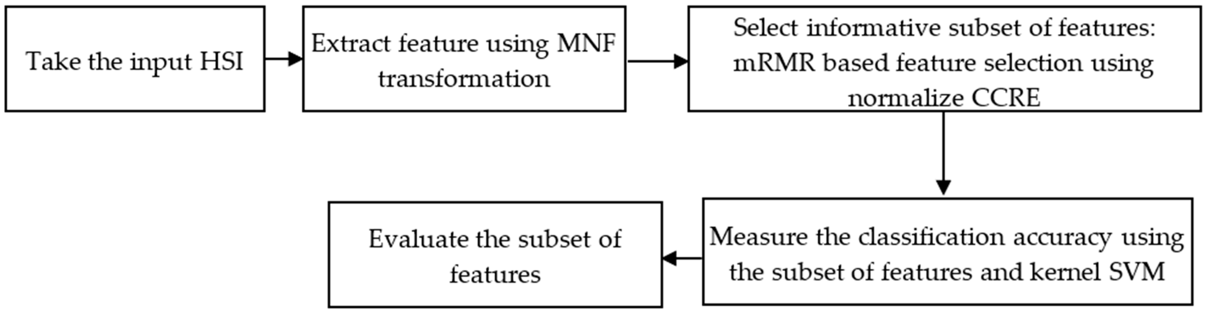
3. Proposed Methodology

There are two primary phases in the proposed feature reduction process: (i) feature extraction through the implementation of the classical MNF on the complete HSI; and (ii) feature selection through the measurement of normalizing CCRE-based mRMR criteria on the transformed features of the HSI. Figure 1 illustrates the practical steps of our proposed method.

3.1. mRMR-Driven CCRE-Based Feature Selection

When deciding which features are most useful, the CCRE value in Equation (12) is taken into account. Using a comparison between the newly generated features from MNF component, Z_i, and the available training class labels, C, CCRE is able to isolate the subset of features that were most important. Therefore, the feature that is calculated to be the most informative is as [31]:

$$V=Ma{x}_{i\in p}{C}_{CCRE}\left(Z_i,C\right),$$

(14)

where V is the most informative classification feature (maximum CCRE value) that was given to S (the number of features that were chosen). This ranked the MNF components, with the possibility that the first few components are the most useful for classification. However, there may be redundancy in the features chosen using Equation (14). Overall, the selected features should be as relevant as possible while being as redundant as possible. The greedy strategy can be utilized to select the (k + 1)^th feature; then, it can be assigned to the subsets that have already been chosen. As such, the mRMR algorithm can be used to determine the model that was picked for subspace detection as:

$$G\left(Z_i,k\right)=\left[C_{CCRE}\left(Z_i,C\right)-\frac{1}{\left|S\right|}{{\displaystyle \sum }}_{i,j\in S}{C}_{CCRE}\left(Z_i,Z_j\right)\right],Z_i\not\subset S.$$

(15)

In Equation (15), S represent the subset of selected feature, Z_i is the current features extracted from MNF, k denotes the number of features to be selected for the feature space S, C signifies the ground truth image of the HSI, and Z_j represents the already selected feature in the feature space, S.

3.2. Improved Feature Selection

(i) Using normalized CCRE: The values of CCRE are not constrained to a particular limit. Direct application of the $G\left(Z_i, k\right)$ in the aforementioned method is complicated by the fact that it is sensitive to the entropy of two variables and does not have a fixed range of validity. The quality of a given CCRE value is evaluated by comparing it to the range [0, 1] [32,33]. The normalized CCRE can be defined as:

$${\widehat{C}}_{CCRE}\left(Z,C\right)=\frac{C_{CCRE}\left(Z,C\right)}{\sqrt{C_{CCRE}\left(Z\right)C_{CCRE}\left(C\right)}}$$

(16)

We propose nCCRE_mRMR, utilizing the normalized CCRE in Equation (16). Accordingly, the subset of features using our proposed method can be defined as:

$$\widehat{G}\left(Z_i,k\right)=\left[{\widehat{C}}_{CCRE}\left(Z_i,C\right)-\frac{1}{\left|S\right|}{{\displaystyle \sum }}_{i,j\in S}{\widehat{C}}_{CCRE}\left(Z_i,Z_j\right)\right],Z_i\not\subset S.$$

(17)

The observation is made that the (k + 1)^th feature to be added to the target subspace of features, S, should have the largest value of $\widehat{\mathrm{G}}\left(Z_i,k\right)$.

(ii) Discard Negative values: Using Equation (17), the largest value of the difference might be less than zero, resulting in the chosen features being different from the previously picked characteristics, which is undesirable. As a result, in this study, $\widehat{\mathrm{G}}\left(Z_i,k\right)$ was assumed to be positive, i.e., $\widehat{\mathrm{G}}\left(Z_i,k\right)>0$. If the greatest difference value is not positive, it might mean that there are no longer any desirable characteristics, and that the informative subspace has grown to its specified width.

(iii) Remove the noisy features: The formula described in Equation (17) is likely to be used to choose undesirable features. The selected features are thus only weakly related to the target when the largest difference value derives from two tiny values. The user-defined threshold (T) is introduced as a means of avoiding complications (if ${\widehat{C}}_{CCRE}\left(Z_i,C\right)<T$, remove Z_i). The preprocessing stage applies the user-defined threshold, T, to condense the searching space for the greedy technique and eliminate the noisy feature. An outline of the suggested hybrid feature reduction method’s algorithm is provided below. Now, the selected set S contains the most informative features. The proposed feature reduction methodology is illustrated in Algorithm 1.

Algorithm 1 MNF-nCCREmRMR

(Y is the original HSI data, Z represents the transform MNF components, C is the ground truth image, T defines a user-defined threshold, and S represents the final subsets of n number of features.)     i. Start ($Z$: the projected data matrix of original HSI, Y)    ii. Evaluate ${\widehat{C}}_{CCRE}$(Zi, C) and utilize T, if ${\widehat{C}}_{CCRE}$(Zi, C) < T   iii. Set, $S_0$= {Ф}   iv. Set$S_1=S_0\cup Z_j$, where $Z_j$ is first feature utilizing Equations (14) and (16)    v. Apply steps (vi) and (vii) until the S contains n features   vi. Update $S$ by utilizing Equation (17)  vii. OutputS as the subsets of effective features

4. Experimental Setup and Analysis

4.1. Remote Sensing Data Sets

For experimental analysis, we used three HSI datasets publicly available and broadly used for HSI classification, i.e., AVIRIS IP, HYDICE Washington DC Mall (WDM), and ROSIS Pavia University (PU). Detailed descriptions of these datasets are given below.

4.1.1. AVIRIS IP Dataset

NASA’s AVIRIS sensor captured the IP dataset in June 1992, which consists of 220 imaging bands [34]. The ground truth image, which is made up of sixteen classes and has a dimension of 145 by 145 pixels, contains the dataset. Furthermore, the data have a 0.1 µm spectral resolution. We excluded the classes “Oats” and “Grass/Pasture mowed” from this experiment for their insufficient training and testing samples. Figure 2 presents the IP false-color RGB and ground truth image.

4.1.2. HYDICE WDM Dataset

The WDM data collection comprises 191 image bands, and each band consists of 1280 × 307 pixels. The HYDICE sensor captured the data in 1995 over the WDM. In the scenario depicted by the ground truth image, there are a total of seven distinct classes [35]. We have not employed “paths” in this study because the training data are insufficient. Figure 3 presents the WDM false-color RGB and ground truth image.

4.1.3. ROSIS PU Dataset

The ROSIS optical sensor was utilized to gather the PU dataset from the University of Pavia’s urban environment in Italy. A spatial resolution of 1.3 m per pixel and an image size of 610 × 610 were used in this his [36]. The acquired image contains 103 data channels (with a spectral range from 0.43 μm to 0.86 μm). A false-color composite of the image appears in Figure 4a, whereas nine ground-truth classes of interest are depicted in Figure 4b.

Table 1. Summary of the HSI datasets.

Name of the Dataset	Capturing Sensor	$\mathit{P}$	Wavelength Range (nm)	$\mathit{H}$	$\mathit{W}$	Ground Classes	Ground Sampling Distance (m)
IP	AVIRIS	220	400–2500	145	145	16	20
WDM	HYDICE	191	400–2400	1280	307	7	3
PU	ROSIS	103	430–860	610	610	9	1.3

reviews the key features of all the three datasets.

4.2. Analysis of Feature Extraction and Feature Selection

During feature extraction, the MNF technique generates new features using the transformation principles. In order to enhance the subset of features, features are chosen utilizing the normalized CCRE on newly generated features. It is possible to select the noisy feature using Equation (14). Furthermore, two weak MNF components might yield a large variation, and the algorithm can pick a useless component that is weakly connected to the ground truth image. We implemented a user-defined threshold T to prevent the use of less informative features in classification. The advantage of using T is that throughout the preprocessing steps, it first rejects noisy features. As a result, there is a reduced possibility of selecting a noisy features, and the order of the chosen features is apparent. For assessing the robustness of the proposed approach, we compared it to MNF, CCRE, MNF-MI, and MNF-CCRE methods.

Table 2. Description of different studied and proposed methods.

Acronym	Method Type	Information Used for Dimension Reduction	Main Steps
PCA	Conventional	Spectral	i. Obtain the covariance matrix of mean adjusted data.  ii. Apply the Eigen decomposition operation on the covariance matrix. iii. Calculate the projection matrix.
MNF	Conventional	Spectral	i. Whiten the noise.  ii. Obtain the covariance matrix of noise adjusted data. iii. Calculate the projection matrix.
MI	Conventional	Spatial	i. Calculate the MI of individual spectral bands and ground truth image. ii. Sort the image bands based on MI values.
CCRE	Conventional	Spatial	i. Calculate the CCRE of individual spectral bands and ground truth image. ii. Sort the image bands based on CCRE values.
nCCRE	Conventional	Spatial	i. Calculate the normalized CCRE of individual spectral bands and ground truth image. ii. Sort the image bands based on normalized CCRE values.
PCA-MI	Hybrid	Spectral-spatial	i. Calculate the projection matrix using the PCA approach.  ii. Calculate the MI values between the PCA bands and ground truth image. iii. Select the informative features according to the MI values.
PCA-CCRE	Hybrid	Spectral-spatial	i. Calculate the projection matrix using the PCA approach.  ii. Calculate the CCRE values between the PCA bands and ground truth image. iii. Select the informative features according to the CCRE values.
MNF-MI	Hybrid	Spectral-spatial	i. Calculate the projection matrix using the MNF approach.  ii. Calculate the MI values between the MNF bands and ground truth image. iii. Select the informative features according to the MI values.
MNF-CCRE	Hybrid	Spectral-spatial	i. Calculate the projection matrix using the MNF approach.  ii. Calculate the CCRE values between the MNF bands and ground truth image. iii. Select the informative features according to the CCRE values.
MNF-nCCRE	Hybrid	Spectral-spatial	i. Calculate the projection matrix using the MNF approach.  ii. Calculate the normalized CCRE values between the MNF bands and ground truth image. iii. Select the informative features according to the normalized CCRE values.
MNF-nCCREmRMR	Hybrid	Spectral-spatial	i. Calculate the projection matrix using the MNF approach. ii. Select the informative features using the proposed feature selection method.

outlines the abbreviations associated with the stated and different methods studied. For all studied and proposed methods, the order of the ranked features is presented in

Table 3. The order of selected features for AVIRIS IP dataset.

Method	Orders of the Selected Features
PCA	PCA Components: 1, 2, 3, 4, 5, 6, 7, 8, 9, 10
MNF	MNF Components: 1, 2, 3, 4, 5, 6, 7, 8, 9, 10
MI	HSI Bands: 29, 22, 23, 32, 188, 128, 43, 192, 24, 25
CCRE	HSI Bands: 22, 29, 28, 32, 27, 26, 30, 33, 25, 24
nCCRE	HSI Bands: 32, 22, 34, 188, 191, 26, 23, 30, 28, 188
PCA-MI	PCA Components: 1, 3, 4, 7, 8, 5, 6, 11, 15, 12
PCA-CCRE	PCA Components: 1, 3, 2, 5, 9, 8, 11, 7, 16, 13
MNF-MI	MNF Components: 2, 5, 4, 3, 6, 7, 8, 9, 10, 11
MNF-CCRE	MNF Components: 3, 2, 6, 4, 5, 8, 7, 10, 9, 15
MNF-nCCRE	MNF Components: 2, 3, 5, 11, 8, 13, 16, 12, 9, 10
MNF-nCCREmRMR	MNF Components: 2, 4, 6, 4, 5, 10, 9, 13, 12, 11

,

Table 4. The order of selected features for HYDICE WDM dataset.

Method	Orders of the Selected Features
PCA	PCA Components: 1, 2, 3, 4, 5, 6, 7, 8, 9, 10
MNF	MNF Components: 1, 2, 3, 4, 5, 6, 7, 8, 9, 10
MI	HSI Bands: 82, 83, 28, 166, 128, 82, 155, 151, 52, 12
CCRE	HSI Bands: 83, 50, 101, 77, 28, 57, 167,165, 51, 82
nCCRE	HSI Bands: 83, 102, 52, 66, 42, 166, 182, 177, 15, 86
PCA-MI	PCA Components: 1, 3, 4, 5, 2, 9, 11, 15, 13, 10
PCA-CCRE	PCA Components: 1, 2, 5, 4, 9, 7, 11, 15, 16, 12
MNF-MI	MNF Components: 2, 5, 4, 3, 6, 1, 191, 14, 18, 11
MNF-CCRE	MNF Components: 2, 3, 4, 5, 1, 6, 7, 19, 18, 12
MNF-nCCRE	MNF Components: 2, 3, 5, 6, 12, 7, 8, 4, 13, 11
MNF-nCCREmRMR	MNF Components: 2, 4, 8, 5, 3, 6, 7, 11, 13, 12

and

Table 5. The order of selected features for ROSIS PU dataset.

Method	Orders of the Selected Features
PCA	PCA Components: 1, 2, 3, 4, 5, 6, 7, 8, 9, 10
MNF	MNF Components: 1, 2, 3, 4, 5, 6, 7, 8, 9, 10
MI	HSI Bands: 102, 103, 98, 101, 95, 96, 97, 88, 99, 100
CCRE	HSI Bands: 103, 102, 100, 99, 86, 88, 96, 97, 92, 83
nCCRE	HSI Bands: 103, 101, 98, 99, 87, 91, 83, 103, 92, 95
PCA-MI	PCA Components: 1, 2, 4, 3, 6, 8, 7, 9, 12, 11
PCA-CCRE	PCA Components: 1, 3, 5, 2, 9, 11, 10, 6, 15, 7
MNF-MI	MNF Components: 2, 3, 4, 6, 5, 11, 9, 10, 8, 12
MNF-CCRE	MNF Components: 2, 3, 4, 5, 7, 8, 13, 11, 16, 9
MNF-nCCRE	MNF Components: 2, 3, 5, 4, 8, 7, 12, 10, 11, 13
MNF-nCCREmRMR	MNF Components: 2, 4, 3, 9, 7, 11, 15, 16, 10, 8

for all three datasets, respectively. The proposed method (MNF-nCCRE_mRMR), as shown in Table 3, ranks MNF component two (MNF-C: 2) and MNF component four (MNF-C: 4) as the top two features, in contrast to the traditional MNF method, which ranks MNF component one (MNF-C: 1) and MNF component two (MNF-C: 2) as the first and second-ranked features, respectively. Figure 5 provides a graphic representation of the first two ranking features of MNF, MNF-MI, and MNF-CCRE, as well as the proposed approach of the AVIRIS image. The illustration demonstrates how the suggested approach improves the effectiveness of the chosen characteristics and is more visually appealing than the other approaches used.

4.3. Parameters Tuning for Classification

To evaluate the effectiveness of the chosen features, we used the KSVM classifier with the Gaussian (RBF) kernel to classify the HSIs. In the classifier, we used a grid search strategy based on tenfold cross-validation to determine the optimal values for the cost parameter, C, and the kernel width, γ [37]. The complete parameter tuning results for all the studied and proposed methods on the three datasets are presented in

Table 6. Parameter tuning results using tenfold cross-validation for the AVIRIS IP dataset.

Method	Best C	Best γ	Training Accuracy
PCA	2.8	3	98.55
MNF	5	2.9	94.63
MI	3	2	81.3
CCRE	2.7	3.7	89.31
nCCRE	8	2.2	88.32
PCA-MI	10	1.3	96.98
PCA-CCRE	7	1	98.81
MNF-MI	10	2.7	97.53
MNF-CCRE	8	2.8	97.89
MNF-nCCRE	5	2	98.91
MNF-nCCREmRMR	2.1	1.2	99.85

,

Table 7. Parameter tuning results using tenfold cross-validation for the HYDICE WDM dataset.

Method	Best C	Best γ	Training Accuracy
PCA	10	2.9	97.55
MNF	4	2.1	98.43
MI	2	3.7	85.61
CCRE	3	2	91.32
nCCRE	7	1.2	92.58
PCA-MI	8	2	98.58
PCA-CCRE	10	2.1	98.93
MNF-MI	8	2.8	99.09
MNF-CCRE	5	3	99.18
MNF-nCCRE	3	0.5	99.88
MNF-nCCREmRMR	2.2	1.8	99.95

and

Table 8. Parameter tuning results using tenfold cross-validation for the ROSIS PU dataset.

Method	Best C	Best γ	Training Accuracy
PCA	10	3	95.85
MNF	5	1.9	95.63
MI	2	2.7	87.86
CCRE	8	2.9	88.39
nCCRE	10	0.2	88.81
PCA-MI	8	2.5	97.98
PCA-CCRE	10	2.9	97.89
MNF-MI	1.2	3	98.06
MNF-CCRE	10	3	98.43
MNF-nCCRE	8	1.5	99.24
MNF-nCCREmRMR	5	2.2	99.91

, respectively. In particular, we obtained the optimal parameters C = 2.9 and γ = 0.5 for the AVIRIS dataset, C = 2.4 and γ = 2.1 for the HYDICE dataset, and C = 2.8 and γ = 3 for the ROSIS PU HSI.

4.4. Classification Performance Evaluation Metrics

In this study, the performance of the proposed method was assessed using commonly used quality indicators, including overall accuracy (OA), average accuracy (AA), the Kappa coefficient, and the F1 score. The proportion of all correctly categorized pixels is what the OA calculates; it can be calculated as follows:

$$\mathrm{OA}={\displaystyle \sum }_{i=1}^C\frac{A_{ii}}{B}$$

(18)

The confusion matrix represented by A is determined by contrasting the classification map with the actual image. The number of classes is denoted by the letter C in this equation. A_ii represents the number of samples in class i that are classified as class i, while B represents the total number of test samples. AA stands for the average value of the proportion of pixels in each class that have been correctly classified. This value is derived as follows:

$$\mathrm{AA}=\frac{{{\displaystyle \sum }}_{i=1}^C\left(A_{ii}/{{\displaystyle \sum }}_{i=1}^C{A}_{i+}\right)}{C},$$

(19)

where A_ii stands for the total number of samples belonging to class i and classified as class i, and A_i+ represents the total number of samples as classified as class i. The Kappa coefficient computes the proportion of classified pixels adjusted for the number of agreements predicted only by chance. It indicates how much better the categorization performed than the likelihood of randomly assigning pixels to their correct categories and can be calculated using the notation used in Equations (18) and (19) as:

$$\mathrm{Kappa}=\frac{\left(B{{\displaystyle \sum }}_{i=1}^C{A}_{ii}-{{\displaystyle \sum }}_{i=1}^C(A_{i+})\left(A_{+i}\right)\right)}{\left(B^2-{{\displaystyle \sum }}_{i=1}^C{{\displaystyle \sum }}_{i=1}^C(A_{i+})\left(A_{+i}\right)\right)},$$

(20)

where A_+i represents the total number of actual samples of class i. Now, the F1 score is calculated as follows:

$$\mathrm{F}1 \mathrm{score}=\frac{2 \times \mathrm{Precision} \times \mathrm{Recall}}{\mathrm{Precision}+\mathrm{Recall}},$$

(21)

where the precision and recall can be calculated as follows:

$$\mathrm{Precision}=\frac{\mathrm{TP}}{\mathrm{TP}+\mathrm{FP}} \mathrm{and} \mathrm{Recall}=\frac{\mathrm{TP}}{\mathrm{TP}+\mathrm{FN}}.$$

(22)

In Equation (22), TP, FP, and FN denote the number of true positive, false positive, and false negative classification of the testing samples of multiple classes.

4.5. Classification Results on the AVIRIS IP Dataset

In this experiment, we took approximately 50% samples of each class as the training set and 50% samples as the testing set from a total of 2401 samples. The information regarding the samples utilized for both training and testing is presented in Table S1. As shown in Figure 2, the ground-truth image served as the basis for selecting both the training and testing samples to be used in the classification process. We calculated the OA of AVIRIS data without feature extraction and feature selection, and found 66.85% using the first ten features. This result provides motivation to reduce the number of features used in HSI classification.

Table 9. Classification performance measure (%) on the AVIRIS IP HSI.

Class	PCA	MNF	MI	CCRE	nCCRE	PCA-MI	PCA-CCRE	MNF-MI	MNF-CCRE	MNF-nCCRE	MNF-nCCREmRMR
Alfalfa	88.89	88.89	75.00	61.54	76.19	94.12	88.89	90.00	90.00	94.12	90.00
Wheat	86.84	90.41	83.58	85.71	80.49	86.84	88.00	95.65	95.65	97.06	95.65
Bldge-Grass	90.00	94.74	72.00	36.73	90.00	90.48	86.36	94.74	94.74	100.00	100.00
Soybean-min	97.63	97.70	79.31	71.32	80.95	97.08	97.08	98.84	98.87	97.16	98.87
Stone-Steel	76.00	94.74	76.00	62.50	76.00	79.17	76.00	95.24	96.55	89.29	100.00
Soybean-no till	92.71	91.49	57.85	90.91	61.07	92.71	94.68	98.90	98.90	96.81	98.94
Grass/Pasture	97.01	82.22	80.65	36.18	96.49	97.01	98.48	82.22	88.10	97.30	88.10
Corn-no till	78.95	77.59	64.81	56.45	64.81	90.00	90.00	79.37	90.91	90.57	90.91
Soybean Clean	64.71	52.38	52.38	52.38	52.38	64.71	57.89	64.71	72.22	86.67	75.00
Corn-min	83.33	93.75	71.43	71.43	73.33	83.33	90.16	94.20	94.20	94.03	98.48
Hay-windrowed	95.17	92.67	48.08	90.09	49.26	95.17	94.52	95.86	99.29	97.96	100.00
Woods	100.00	99.58	93.78	95.15	93.78	100.00	99.22	99.58	99.59	99.61	99.59
Grass/Trees	82.91	96.08	82.46	91.59	90.38	86.73	86.73	96.08	98.00	95.15	100.00
Corn	97.40	98.61	78.95	90.91	90.91	98.68	98.70	98.68	98.68	98.70	98.70
AA	87.97	89.35	72.59	70.921	76.86	89.72	89.05	91.7233	93.98	95.31	95.30
OA	92.38	93.04	72.95	75.126	75.96	93.55	93.63	94.90	96.72	96.90	97.44
KAPPA	91.42	92.17	69.66	72.33	73.09	92.73	92.82	94.3	96.3	96.50	97.10
F1 Score	88.07	89.13	73.53	73.20	77.31	89.33	89.04	91.90	94.7	94.70	96.3

shows the values of the OA, AA, Kappa, and F1 score of each method. The proposed technique has the highest OA, AA, and Kappa values, as shown in the table. This table demonstrates that the proposed MNF-nCCREmRMR approach performs better than the state-of-the-art methods on every single criterion used to evaluate performance. The two-dimensional line graphs presented in Figure 6 show the comparison of the proposed and studied methods in a more meaningful way using the OA versus the number of ranked features. As the number of features increases, the OA increases too.

4.6. Classification Results on the HYDICE WDM Dataset

In this experiment, we have taken around 30% samples of each class as training set and 70% samples as testing set from a total of 5154 samples. Table S2 contains a representation of the information regarding the samples used for both training and testing. As shown in Figure 3, the ground-truth image is used to choose both the training samples and the testing samples for classification.

Table 10. Classification performance measure (%) on the HYDICE WDM HSI.

Class	PCA	MNF	MI	CCRE	nCCRE	PCA-MI	PCA-CCRE	MNF-MI	MNF-CCRE	MNF-nCCRE	MNF-nCCREmRMR
Shadow (C1)	90.91	58.54	88.24	72.73	90.63	96.77	97.06	58.00	71.74	97.06	100.00
Tree (C2)	97.08	97.24	92.14	95.17	92.63	97.09	97.09	98.34	99.23	98.49	100.00
Roof (C3)	92.14	73.55	88.24	61.24	82.69	88.36	97.74	82.64	89.47	97.74	98.48
Water (C4)	92.38	95.41	82.90	95.36	87.11	93.27	93.33	97.94	98.92	96.55	98.77
Street (C5)	93.85	86.77	93.77	86.63	92.44	93.85	94.10	93.67	96.84	93.66	99.74
Grass (C6)	86.14	93.01	80.35	78.82	83.09	92.55	92.59	96.77	96.88	99.23	100.00
AA	92.08	84.09	87.61	81.66	88.10	93.65	95.32	87.89	92.18	97.12	99.50
OA	92.50	93.36	87.27	87.67	88.65	94.54	94.97	96.12	97.56	97.93	99.71
KAPPA	89.57	90.73	82.27	82.93	84.18	92.37	92.97	94.60	96.60	97.06	99.60
F1 Score	92.41	84.84	87.87	81.75	89.28	93.55	95.38	90.56	94.44	97.24	99.44

shows the values of the OA, AA, Kappa, and F1 score of each method. Performing the equivalent number of selected features, we find the OA of 99.71% by the proposed MNF-nCCRE_mRMR method. This table demonstrates that the proposed MNF-nCCRE_mRMR approach performs better than the state-of-the-art methods on every single criterion used to evaluate performance. In addition, the line graphs presented in Figure 7 shows the comparison of the proposed over the others. It can be seen that the overall classification accuracy increases with the increase in the ranked features.

4.7. Classification Results on the ROSIS PU Dataset

For the ROSIS PU dataset, we took approximately 17% samples of each class as training set and 83% samples as testing set from a total of 20,075 samples. The detailed information of the training and testing samples is presented in Table S3. The ground-truth image is used to select the training and testing samples for classification, as shown in Figure 4.

Table 11. Classification performance measure (%) on the ROSIS PU HSI.

Class	PCA	MNF	MI	CCRE	nCCRE	PCA-MI	PCA-CCRE	MNF-MI	MNF-CCRE	MNF-nCCRE	MNF-nCCREmRMR
Asphalt	99.70	96.89	93.42	93.45	93.46	99.71	99.71	99.71	99.27	99.71	99.70
Meadows	90.34	92.25	73.73	75.29	75.29	99.32	99.41	99.86	97.70	99.89	100
Gravel	86.53	87.74	82.10	82.08	82.08	88.24	88.24	89.73	99.87	89.77	89.83
Tree	83.10	83.10	67.80	67.89	80.39	84.09	84.09	84.71	92.84	83.72	84.03
metal sheets	90.85	93.01	68.23	68.47	69.04	98.55	98.56	95.13	92.18	92.18	93.45
Bare soil	88.01	88.05	62.60	62.60	64.10	91.41	94.71	96.04	96.29	99.62	100
Bitumen	99.52	99.36	87.89	91.82	91.88	99.36	99.36	99.52	99.52	100.00	100
Blocking Bricks	85.57	87.65	69.30	69.30	69.30	95.42	94.68	94.68	98.08	98.09	100
Shadow	86.96	86.96	86.96	86.96	86.96	100.00	100.00	100.00	100.00	100.00	100
AA	90.06	90.56	76.89	77.54	79.17	95.12	95.42	95.49	97.31	95.89	96.33
OA	90.87	91.35	75.48	76.13	76.90	96.12	96.58	96.89	97.62	97.88	98.35
KAPPA	88.88	89.46	70.11	70.94	71.86	95.28	95.84	96.22	97.09	97.42	98.00
F1 Score	90.47	91.24	76.94	77.99	79.21	95.66	95.64	95.87	96.62	96.21	97.39

shows the results of the OA, AA, Kappa, and F1 score of each method. Performing on the same number of selected features, we found a classification accuracy of 98.35% by the proposed MNF-nCCRE_mRMR method. This table also demonstrates that the proposed MNF-nCCRE_mRMR method outperformed all the performance measurement metrics. Based on the two-dimensional line graph presented in Figure 8, it can be seen that as the number of features increases, the overall classification accuracy also increases.

We next calculated the OA on the three datasets in various numbers of training and testing ratios to confirm the robustness of the suggested feature extraction techniques in comparison to the investigated state-of-the-art feature reduction techniques.

Table 12. OA measure using three different training: testing ratios on the three HSI datasets.

Training Size	Dataset	PCA	MNF	MI	CCRE	nCCRE	PCA-MI	PCA-CCRE	MNF-MI	MNF-CCRE	MNF-nCCRE	MNF-nCCREmRMR
10%	IP	89.94	89.29	67.39	67.95	68.18	89.21	90.12	90.09	91.10	91.39	93.21
	WDM	89.89	90.08	84.57	85.17	85.31	91.85	91.89	94.38	95.75	95.56	97.39
	PU	90.05	90.15	74.14	75.19	74.08	95.32	95.51	94.29	96.14	96.29	97.79
20%	IP	89.28	90.50	68.57	70.18	70.89	90.54	91.39	91.94	94.39	94.67	95.39
	WDM	91.41	91.95	86.35	86.74	86.94	93.12	93.58	95.08	96.47	96.25	98.24
	PU	90.87	91.35	75.48	76.13	76.90	96.12	96.58	96.89	97.62	97.88	98.35
30%	IP	91.23	91.58	70.56	72.61	72.97	91.86	92.01	93.80	95.22	95.94	96.92
	WDM	92.50	93.36	87.27	87.67	88.65	94.54	94.97	96.12	97.56	97.93	99.71
	PU	91.09	91.95	76.20	77.07	77.61	96.79	96.96	97.09	97.93	98.05	98.94

shows the OA of the three datasets in 10%, 20%, and 30% of training samples. The results also reveal that the proposed method for feature extraction was better that the investigated state-of-the-art feature reduction methods for each of the three HSI datasets. On the other hand, we tested the investigated and proposed methods utilizing the three classifiers (Naïve Bayes classifier, decision tree classifier, and SVM) for three datasets are presented in

Table 13. Classification performance measure (%) on the AVIRIS IP HSI for different dimension reduction methods and classification methods.

Classifiers	Class	PCA	MNF	MI	CCRE	nCCRE	PCA-MI	PCA-CCRE	MNF-MI	MNF-CCRE	MNF-nCCRE	MNF-nCCREmRMR
Naïve Bayesian Classifier	AA	80.02	83.65	68.59	69.921	67.86	83.72	86.05	87.38	87.69	88.50	88.05
	OA	81.38	83.01	67.95	68.126	67.96	82.55	86.17	86.41	87.04	88.20	89.04
	KAPPA	82.33	84.24	67.66	69.33	68.09	82.73	86.09	88.63	87.02	87.31	88.89
	F1 Score	80.20	83.32	68.53	68.20	68.31	81.33	86.04	86.82	87.27	86.89	87.39
Decision Tree	AA	85.54	85.24	70.59	73.921	75.27	87.24	88.34	90.91	92.57	93.24	93.87
	OA	88.22	87.12	70.95	73.126	75.31	88.91	87.87	91.27	93.35	93.54	94.68
	KAPPA	89.06	85.68	71.66	74.01	74.28	87.34	89.68	91.39	92.64	92.21	93.25
	F1 Score	84.07	86.72	70.53	73.20	72.30	87.27	88.18	90.28	91.18	93.31	92.58
SVM	AA	87.97	89.35	72.59	70.921	76.86	89.72	89.05	91.7233	93.98	95.31	95.30
	OA	92.38	93.04	72.95	75.126	75.96	93.55	93.63	94.90	96.72	96.90	97.44
	KAPPA	91.42	92.17	69.66	72.33	73.09	92.73	92.82	94.3	96.3	96.50	97.10
	F1 Score	88.07	89.13	73.53	73.20	77.31	89.33	89.04	91.90	94.7	94.70	96.3

,

Table 14. Classification performance measure (%) on the HYDICE WDM HSI for different dimension reduction methods and classification methods.

Classifiers	Class	PCA	MNF	MI	CCRE	nCCRE	PCA-MI	PCA-CCRE	MNF-MI	MNF-CCRE	MNF-nCCRE	MNF-nCCREmRMR
Naïve Bayesian Classifier	AA	82.09	82.69	66.87	67.58	67.34	86.54	86.97	88.37	87.22	88.41	88.57
	OA	84.64	85.72	68.39	69.29	69.38	88.23	88.56	89.21	88.19	89.57	89.86
	KAPPA	82.64	83.66	65.28	67.64	68.39	86.35	87.58	86.41	85.31	87.24	88.94
	F1 Score	81.47	81.47	65.44	67.38	67.46	83.57	86.34	87.85	83.54	87.28	89.07
Decision Tree	AA	90.29	88.43	82.58	83.34	84.98	93.39	91.58	92.87	93.39	94.09	96.65
	OA	91.07	90.97	84.24	84.71	85.34	95.47	93.42	94.49	95.27	95.33	97.39
	KAPPA	88.65	87.29	80.39	82.98	83.48	93.74	91.79	92.39	92.74	95.03	96.74
	F1 Score	88.47	86.98	79.73	82.75	81.39	94.09	90.98	91.85	92.45	94.17	96.29
SVM	AA	92.08	84.09	87.61	81.66	88.10	93.65	95.32	87.89	92.18	97.12	99.50
	OA	92.50	93.36	87.27	87.67	88.65	94.54	94.97	96.12	97.56	97.93	99.71
	KAPPA	89.57	90.73	82.27	82.93	84.18	92.37	92.97	94.60	96.60	97.06	99.60
	F1 Score	92.41	84.84	87.87	81.75	89.28	93.55	95.38	90.56	94.44	97.24	99.44

and

Table 15. Classification performance measure (%) on the ROSIS PU HSI for different dimension reduction methods and classification methods.

Classifiers	Class	PCA	MNF	MI	CCRE	nCCRE	PCA-MI	PCA-CCRE	MNF-MI	MNF-CCRE	MNF-nCCRE	MNF-nCCREmRMR
Naïve Bayesian Classifier	AA	80.99	78.18	62.22	61.31	64.22	83.10	82.39	84.41	84.44	94.39	85.99
	OA	81.08	80.98	64.25	65.87	67.57	85.47	85.45	85.17	86.48	86.27	87.87
	KAPPA	80.45	79.45	61.34	66.20	60.97	82.36	82.64	83.36	83.60	84.21	84.95
	F1 Score	79.33	78.33	61.18	64.39	61.33	81.44	81.22	82.95	83.25	81.59	82.33
Decision Tree	AA	86.19	86.3	70.09	71.47	71.31	91.33	92.14	92.31	93.19	94.69	95.29
	OA	88.91	88.32	73.71	74.34	74.97	93.27	94.81	94.52	94.24	96.08	96.28
	KAPPA	85.33	85.70	70.01	70.66	70.54	91.47	92.34	92.47	93.37	95.38	95.08
	F1 Score	83.97	85.44	69.95	71.01	70.11	90.65	91.19	92.39	92.85	94.29	94.27
SVM	AA	90.06	90.56	76.89	77.54	79.17	95.12	95.42	95.49	97.31	95.89	96.33
	OA	90.87	91.35	75.48	76.13	76.90	96.12	96.58	96.89	97.62	97.88	98.35
	KAPPA	88.88	89.46	70.11	70.94	71.86	95.28	95.84	96.22	97.09	97.42	98.00
	F1 Score	90.47	91.24	76.94	77.99	79.21	95.66	95.64	95.87	96.62	96.21	97.39

, respectively. From these tables’ data, we can conclude that the proposed methods outperform the studied methods.

4.8. Features Scatter Plot Analysis

Here, we consider the feature space analysis approach using the scatter plot of the first two selected features to evaluate the robustness of the proposed method (MNF-nCCRE_mRMR). Figure 9 depicts the feature space for the AVIRIS IP dataset, utilizing the conventional approaches such as MNF, MNF-MI, MNF-CCRE, and proposed method. We used eight classes in the scatter plot to keep things simple. In this case, the standard MNF and MNF-MI methods exhibited greater class overlap, as shown in Figure 9a,b. As opposed to these studied methods, the proposed method MNF-nCCRE_mRMR demonstrates that the classes are more visually separable. Similarly, the feature space for the traditional MNF, MNF-MI, and MNF-CCRE, and the suggested approach on the WDM HYDICE dataset, is also depicted in Figure 10. As shown in Figure 10a,b, the classes are more intimately connected, but in the proposed method shown in Figure 10d, the class samples are more distinguishable than in the investigated methods. Additionally, it demonstrates how applying normalized CCRE with the mRMR approach to MNF data enhances the dominance of the selected features.

4.9. Extended Analysis

Each method’s execution time is analyzed and listed in this section for comparison. On a desktop computer running the Microsoft Windows 10 operating system and powered by an Intel Core i5 3.2 GHz processor, the experiments were carried out using MATLAB R2014b.

Table 16. The computational time (in second) of each method on AVIRIS IP, HYDICE WDM, and ROSIS PU datasets.

Dataset	Stage	PCA	MNF	MI	CCRE	PCA-MI	PCA-CCRE	MNF-MI	MNF-CCRE	MNF-nCCREmRMR
AVIRIS IP	Transformation	0.11	0.12	—	—	0.11	0.11	0.12	0.12	0.12
	Feature Selection	—	—	1.56	1.38	1.51	1.37	1.6	1.45	1.58
	Total Cost	0.11	0.12	1.56	1.38	1.62	1.48	1.72	1.57	1.7
HYDICE WDM	Transformation	0.17	0.18	—	—	0.17	0.17	0.19	0.19	0.19
	Feature Selection	—	—	2.1	1.83	2.40	0.83	2.6	1.95	2.1
	Total Cost	0.17	0.18	2.1	1.83	2.57	2.0	2.79	2.14	2.29
ROSIS PU	Transformation	0.12	0.10	—	—	0.12	0.12	0.10	0.10	0.10
	Feature Selection	—	—	1.88	1.49	1.91	1.52	2.1	1.6	1.78
	Total Cost	0.12	0.10	1.88	1.49	2.03	1.64	2.2	1.7	1.88

presents the execution time of each method for different datasets, from which it can be seen that MNF-nCCRE_mRMR is computationally comparable with the existing methods. In addition, the robustness of the proposed method MNF-nCCRE_mRMR for the multiclass classification was assessed using the error matrices. Tables S4–S6 show the error matrices using the AVIRIS IP, HYDICE WDM, and ROSIS PU datasets, respectively. All three error matrices illustrate that almost all classes are correctly predicted except very few of them by the proposed method.

5. Conclusions

This study proposes a dimension reduction strategy that combines feature extraction and feature selection in order to find a relevant subset of characteristics for efficient HSI classification. We specifically made use of the widely utilized feature extraction technique MNF and the information theoretic approach CCRE for feature selection. The normalized CCRE was employed alongside the mRMR-driven feature selection criterion to enhance the quality of the chosen feature. The KSVM classifier was used to analyze the performance of the produced feature subsets on three real HSIs. The testing results showed a considerable improvement in the quality of the selected features and classification accuracy as well. The results manifest that applying normalized CCRE to the MNF data with mRMR criteria results in the subsets of informative features. The experiments also manifest that, in comparison to the traditional MNF, feature selection using normalized CCRE after the MNF transformation improves the grade of the selected features. This is the reason that the proposed approach (MNF-nCCRE_mRMR) selected the subset of less noisy features, provided relevant details about the appropriate objects, and ignored the redundant features. The improvement of classification accuracy and feature space analysis demonstrates the robustness of the proposed technique.

Future Work

Although, deep learning is now a trendy tool to analyze HSI but requires a large amount of labeled data, which can be costly and time-consuming. Therefore, in future, MNF-nCCRE_mRMR could be coupled with deep-learning-based approaches to extract both spectral and spatial characteristics of HSIs for further improving the classification performance which overcome the limitation of deep learning based HSI analysis.

References

1. Richards, J.A.; Richards, J. Remote Sensing Digital Image Analysis; Springer: Berlin/Heidelberg, Germany, 1999; Volume 3. [Google Scholar]
2. Campbell, J.B.; Wynne, R.H. Introduction to Remote Sensing; Guilford Press: New York, NY, USA, 2011. [Google Scholar]
3. Chen, Y.; Zhao, X.; Jia, X. Spectral–spatial classification of hyperspectral data based on deep belief network. IEEE J. Sel. Top. Appl. Earth Obs. Remote Sens. 2015, 8, 2381–2392. [Google Scholar] [CrossRef]
4. Islam, M.R.; Ahmed, B.; Hossain, M.A. Feature reduction based on segmented principal component analysis for hyperspectral images classification. In Proceedings of the 2019 International Conference on Electrical, Computer and Communication Engineering (ECCE), Cox’s Bazar, Bangladesh, 7–9 February 2019. [Google Scholar]
5. Jia, X.; Kuo, B.-C.; Crawford, M.M. Feature mining for hyperspectral image classification. Proc. IEEE 2013, 101, 676–697. [Google Scholar] [CrossRef]
6. Tarabalka, Y.; Chanussot, J.; Benediktsson, J.A. Segmentation and classification of hyperspectral images using watershed transformation. Pattern Recognit. 2010, 43, 2367–2379. [Google Scholar] [CrossRef] [Green Version]
7. Lillesand, T.; Kiefer, R.W.; Chipman, J. Remote Sensing and Image Interpretation; John Wiley & Sons: Hoboken, NJ, USA, 2015. [Google Scholar]
8. Hughes, G. On the mean accuracy of statistical pattern recognizers. IEEE Trans. Inf. Theory 1968, 14, 55–63. [Google Scholar] [CrossRef] [Green Version]
9. Islam, M.R.; Hossain, M.A.; Ahmed, B. Improved subspace detection based on minimum noise fraction and mutual information for hyperspectral image classification. In Proceedings of the International Joint Conference on Computational Intelligence, Budapest, Hungary, 2–4 November 2020. [Google Scholar]
10. Islam, R.; Ahmed, B.; Hossain, A. Feature reduction of hyperspectral image for classification. J. Spat. Sci. 2020, 67, 331–351. [Google Scholar] [CrossRef]
11. Luo, G.; Chen, G.; Tian, L.; Qin, K.; Qian, S.-E. Minimum noise fraction versus principal component analysis as a preprocessing step for hyperspectral imagery denoising. Can. J. Remote Sens. 2016, 42, 106–116. [Google Scholar] [CrossRef]
12. Yang, X.; Xu, W.D.; Liu, H.; Zhu, L.Y. Research on dimensionality reduction of hyperspectral image under close range. In Proceedings of the 2019 International Conference on Communications, Information System and Computer Engineering (CISCE), Haikou, China, 5–7 July 2019; pp. 171–174. [Google Scholar]
13. Li, H.; Cui, J.; Zhang, X.; Han, Y.; Cao, L. Dimensionality Reduction and Classification of Hyperspectral Remote Sensing Image Feature Extraction. Remote Sens. 2022, 14, 4579. [Google Scholar] [CrossRef]
14. Kuo, B.C.; Li, C.H. Kernel Nonparametric Weighted Feature Extraction for Classification. In AI 2005: Advances in Artificial Intelligence. AI 2005. Lecture Notes in Computer Science; Zhang, S., Jarvis, R., Eds.; Springer: Berlin/Heidelberg, Germany, 2005; Volume 3809. [Google Scholar] [CrossRef]
15. Gao, H.-M.; Zhou, H.; Xu, L.-Z.; Shi, A.-Y. Classification of hyperspectral remote sensing images based on simulated annealing genetic algorithm and multiple instance learning. J. Central South Univ. 2014, 21, 262–271. [Google Scholar] [CrossRef]
16. Chang, C.-I.; Du, Q. Interference and noise-adjusted principal components analysis. IEEE Trans. Geosci. Remote Sens. 1999, 37, 2387–2396. [Google Scholar] [CrossRef] [Green Version]
17. Fauvel, M.; Chanussot, J.; Benediktsson, J.A. Kernel Principal Component Analysis for the Classification of Hyperspectral Remote Sensing Data over Urban Areas. EURASIP J. Adv. Signal Process. 2009, 2009, 783194. [Google Scholar] [CrossRef] [Green Version]
18. Rodarmel, C.; Shan, J. Principal component analysis for hyperspectral image classification. Surv. Land Inf. Sci. 2002, 62, 115–122. [Google Scholar]
19. Hossain, A.; Jia, X.; Pickering, M. Subspace Detection Using a Mutual Information Measure for Hyperspectral Image Classification. IEEE Geosci. Remote Sens. Lett. 2013, 11, 424–428. [Google Scholar] [CrossRef]
20. Green, A.; Berman, M.; Switzer, P.; Craig, M. A transformation for ordering multispectral data in terms of image quality with implications for noise removal. IEEE Trans. Geosci. Remote Sens. 1988, 26, 65–74. [Google Scholar] [CrossRef] [Green Version]
21. Lixin, G.; Weixin, X.; Jihong, P. Segmented minimum noise fraction transformation for efficient feature extraction of hyperspectral images. Pattern Recognit. 2015, 48, 3216–3226. [Google Scholar] [CrossRef]
22. Guo, B.; Gunn, S.; Damper, R.; Nelson, J. Band Selection for Hyperspectral Image Classification Using Mutual Information. IEEE Geosci. Remote Sens. Lett. 2006, 3, 522–526. [Google Scholar] [CrossRef] [Green Version]
23. Hossain, M.A.; Jia, X.; Pickering, M. Improved feature selection based on a mutual information measure for hyperspectral image classification. In Proceedings of the 2012 IEEE International Geoscience and Remote Sensing Symposium, Munich, Germany, 22–27 June 2012. [Google Scholar]
24. Islam, R.; Ahmed, B.; Hossain, A.; Uddin, P. Mutual Information-Driven Feature Reduction for Hyperspectral Image Classification. Sensors 2023, 23, 657. [Google Scholar] [CrossRef]
25. Uddin, M.P.; Mamun, M.A.; Afjal, M.I.; Hossain, M.A. Information-theoretic feature selection with segmentation-based folded principal component analysis (PCA) for hyperspectral image classification. Int. J. Remote Sens. 2021, 42, 286–321. [Google Scholar] [CrossRef]
26. Das, S.; Routray, A.; Deb, A.K. Fast Semi-Supervised Unmixing of Hyperspectral Image by Mutual Coherence Reduction and Recursive PCA. Remote Sens. 2018, 10, 1106. [Google Scholar] [CrossRef] [Green Version]
27. Machidon, A.L.; Del Frate, F.; Picchiani, M.; Machidon, O.M.; Ogrutan, P.L. Geometrical Approximated Principal Component Analysis for Hyperspectral Image Analysis. Remote Sens. 2020, 12, 1698. [Google Scholar] [CrossRef]
28. Uddin, M.P.; Mamun, M.A.; Hossain, M.A. PCA-based feature reduction for hyperspectral remote sensing image classification. IETE Tech. Rev. 2020, 38, 377–396. [Google Scholar] [CrossRef]
29. Wang, F.; Vemuri, B.C. Non-Rigid Multi-Modal Image Registration Using Cross-Cumulative Residual Entropy. Int. J. Comput. Vis. 2007, 74, 201–215. [Google Scholar] [CrossRef] [Green Version]
30. Rao, M.; Chen, Y.M.; Vemuri, B.C.; Wang, F. Cumulative residual entropy: A new measure of information. IEEE Trans. Inform. Theory 2004, 50, 1220–1228. [Google Scholar] [CrossRef]
31. Peng, H.; Long, F.; Ding, C. Feature selection based on mutual information criteria of max-dependency, max-relevance, and min-redundancy. IEEE Trans. Pattern Anal. Mach. Intell. 2005, 27, 1226–1238. [Google Scholar] [CrossRef] [PubMed]
32. Estevez, P.A.; Tesmer, M.; Perez, C.A.; Zurada, J.M. Normalized Mutual Information Feature Selection. IEEE Trans. Neural Networks 2009, 20, 189–201. [Google Scholar] [CrossRef] [Green Version]
33. Tarabalka, Y.; Benediktsson, J.A.; Chanussot, J. Spectral–Spatial Classification of Hyperspectral Imagery Based on Partitional Clustering Techniques. IEEE Trans. Geosci. Remote Sens. 2009, 47, 2973–2987. [Google Scholar] [CrossRef]
34. Soelaiman, R.; Asfiandy, D.; Purwananto, Y.; Purnomo, M.H. Weighted kernel function implementation for hyperspectral image classification based on Support Vector Machine. In Proceedings of the International Conference on Instrumentation, Communication, Information Technology, and Biomedical Engineering 2009, Bandung, Indonesia, 23–25 November 2009. [Google Scholar]
35. Huang, X.; Han, X.; Zhang, L.; Gong, J.; Liao, W.; Benediktsson, J.A. Generalized Differential Morphological Profiles for Remote Sensing Image Classification. IEEE J. Sel. Top. Appl. Earth Obs. Remote Sens. 2016, 9, 1736–1751. [Google Scholar] [CrossRef] [Green Version]
36. Chen, Z.; Jiang, J.; Jiang, X.; Fang, X.; Cai, Z. Spectral-Spatial Feature Extraction of Hyperspectral Images Based on Propagation Filter. Sensors 2018, 18, 1978. [Google Scholar] [CrossRef] [Green Version]
37. Hsu, C.-W.; Chang, C.-C.; Lin, C.-J. A Practical Guide to Support Vector Classification; National Taiwan University: Taipei, Taiwan, 2003. [Google Scholar]
Figure 1. Overview of the proposed method.
Remotesensing 15 01147 g001
Figure 2. AVIRIS IP data: (a) false color RGB image RGB (50, 27, and 17); (b) ground truth image.
Remotesensing 15 01147 g002
Figure 3. HYDICE WDM data: (a) false color RGB image RGB (50, 52, and 36); (b) ground truth image.
Remotesensing 15 01147 g003
Figure 4. ROSIS PU data: (a) false color RGB image; (b) ground truth image.
Remotesensing 15 01147 g004
Figure 5. Visual representation of first two ranked features of the AVIRIS IP dataset: (a) MNF; (b) MNF-MI; (c) MNF-CCRE; and (d) MNF-nCCREmRMR.
Remotesensing 15 01147 g005
Figure 6. Classification performance measure (%) on the AVIRIS IP HSI.
Remotesensing 15 01147 g006
Figure 7. Classification performance measure (%) on the HYDICE WDM HSI.
Remotesensing 15 01147 g007
Figure 8. Overall classification accuracy versus features for the ROSIS PU dataset.
Remotesensing 15 01147 g008
Figure 9. Feature space on the AVIRIS IP dataset: (a) MNF; (b) MNF-MI; (c) MNF-CCRE; and (d) MNF-nCCREmRMR.
Remotesensing 15 01147 g009aRemotesensing 15 01147 g009b
Figure 10. Feature space on the HYDICE WDM dataset: (a) MNF; (b) MNF-MI; (c) MNF-CCRE; and (d) MNF-nCCREmRMR.
Remotesensing 15 01147 g010