Article

Aboveground Forest Biomass Estimation by the Integration of TLS and ALOS PALSAR Data Using Machine Learning

1
Faculty of Forestry and Wood Sciences, Czech University of Life Sciences, Kamýcká 129, Praha 6–Suchdol, 16500 Prague, Czech Republic
2
Forestry and Ecology Department, Indian Institute of Remote Sensing, Dehradun 248001, India
3
Geomatics Group, Indian Institute of Technology, Roorkee 247667, India
4
International Water Management Institute, 127 Sunil Mawatha, Battaramulla, Colombo 10120, Sri Lanka
5
Faculty of Science, University of Technology Sydney (UTS), 745 Harris St, Ultimo, NSW 2007, Australia
*
Author to whom correspondence should be addressed.
Remote Sens. 2023, 15(4), 1143; https://doi.org/10.3390/rs15041143
Submission received: 20 December 2022 / Revised: 1 February 2023 / Accepted: 6 February 2023 / Published: 20 February 2023
(This article belongs to the Special Issue Remote Sensing and Smart Forestry)

Abstract

:
Forest inventory parameters play an important role in understanding various biophysical processes of forest ecosystems. The present study aims at integrating Terrestrial Laser Scanner (TLS) and ALOS PALSAR L-band Synthetic Aperture Radar (SAR) data to assess Aboveground Biomass (AGB) in the Barkot Forest Range, Uttarakhand, India. The integration was performed to overcome the AGB saturation issue in ALOS PALSAR L-band SAR data for the high biomass density forest of the study area using 13 plots. Various parameters, namely, Gray-Level Co-Occurrence Matrix (GLCM) texture measures, Yamaguchi decomposition components, polarimetric parameters, and backscatter values of HH and HV band intensity, were derived from the ALOS SAR data. However, TLS was used to obtain the diameter at breast height (dbh) and tree height for the sample plots. A total of 23 parameters was retrieved using TLS and SAR data for integration with the LiDAR footprint. The integration was performed using Random Forest (RF) and Artificial Neural Network (ANN). The statistical measures for RF were found to be promising compared with ANN for AGB estimation. The R2 value obtained for the RF was 0.94, with an RMSE of 59.72 ton ha−1 for the predicted biomass value. The RMSE% was 15.92, while the RMSECV was 0.15. The R2 value for ANN was 0.77, with an RMSE of 98.46 ton ha−1. The RMSE% was 26.0, while the RMSECV was 0.26. RF performed better in estimating the biomass, which ranged from 122.46 to 581.89 ton ha−1, while uncertainty ranged from 15.75 to 85.14 ton ha−1. The integration of SAR and LiDAR data using machine learning shows great potential in overcoming AGB saturation of SAR data.

1. Introduction

Forest productivity estimation is important for forest management and ecosystem services monitoring [1]. Destructive sampling techniques are restricted due to labor intensiveness, tedious work, and unsuitability to inaccessible terrain. The emerging techniques of remote sensing are progressively superseding traditional methods. Dataset products from Terrestrial Laser Scanners (TLSs), Airborne Laser Scanning (ALS), Unmanned Aerial Vehicles (UAVs), and other space-borne (GEDI, ICESat-2) platforms, in combination with various machine learning algorithms, have become the preferred options for assessing and mapping aboveground biomasses (AGB) [2,3]. Machine learning algorithms, such as Random Forest (RF) and Artificial Neural Network (ANN) have been used to improve the saturation of biomass value ranges caused by data restrictions [4,5]. The primary aim is to reduce uncertainty in biomass assessment using remote sensing.
Data fusion and integration can play a crucial role in mitigating the uncertainty of biomass [6,7]. Used together, Synthetic Aperture Radar (SAR) and Light Detection and Ranging (LiDAR) overcome the saturation of biomass, with the specific bands of SAR data reducing result biases [8]. Previously, biomass was estimated based on empirical models using PolInsar and PolSAR techniques, which sometimes produced uncertainty of the biomass [9,10]. Subsequently, the use of LiDAR became ubiquitous; however, the occlusion of trees in a plot can occur due to different sets of scanning positions when using ground-based static LiDAR systems [11]. Thus, the resultant uncertainty is also reflected in the results. The detection of trees in forests also depends on the type and density of the forest as well as the scanning positions of the TLS [12].
The estimation of Aboveground Forest Carbon Stocks (AFCS) is always challenging in tropical regions due to structural complexity and high species diversity. ALOS PALSAR texture information resolves AFCS estimation issues in tropical regions [13]. Previously, empirical modeling, such as Extended Water Cloud Models (EWCMs) and Water Cloud Models (WCMs), showed the best correlation among forest parameters and HV backscatter values as well as volume scattering values [14]. The integration of different platform datasets yields promising results as well as complex information. Allometric modeling and biomass calibration and validation can be done using TLS and SAR data [15].
The aim of this study is to investigate other tree attributes derived with TLS and ALOS PALSAR and examine tree attribute correlations with biomass using machine learning. The objective is to overcome biomass saturation over high-density forests using RF and ANN. RF has been used for the estimation of biomass using airborne LiDAR data in moderately dense forests, taking into consideration the correlation between canopy cover and biomass [16,17,18]. Furthermore, other vegetation indices, such as NDVI, have been explored and exhausted to find the best possible correlation and prediction of biomass. Moreover, machine learning algorithms, such as RF and ANN, have been used to predict biomass using different combinations of tree metrics [19,20].

2. Materials and Methods
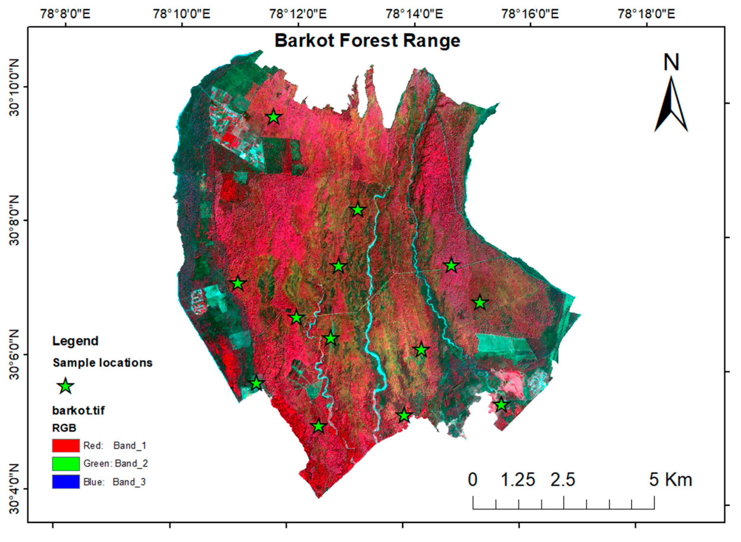
2.1. Study Area

The study area selected for this research was the Barkot Forest Range of Dehradun Forest division, Uttarakhand, India. It lies at a latitude of 30°03′52″ to 30°10′43″N and a longitude of 78°09′49″ to 78°17′09″E. The altitude ranges from 340 m to 560 m above Mean Sea Level (MSL). The study area is in the foothills of the Himalayas and is surrounded by the lesser Himalayas to the north and the Shivalik range to the south. The total area of the forest is 84.96 km2. The forest type is tropical, moist, deciduous. It is dominated by Shorea robusta (Sal), with co-associated tree species such as Mallotus philippensis (Rohini). The topography of the study area varies from plain to undulating. As the depth of the soil increases, the consistency changes from non-sticky and friable to sticky and firm. A lower horizon of the soil profile is sticky, firm, compact, and comparatively hard [21,22]. The study area is shown in Figure 1.

2.2. Above-Ground Biomass Inventory

Tree inventory data were collected by demarcating 13 plots of 31.5 m × 31.5 m. The instruments used for the field data collection were measuring tape, rangefinders, and handheld GPSs. Field sampling was done at the LiDAR footprint using a stratified random sampling method. The sampling locations are shown in Figure 2. Tree parameters, such as dbh and tree height, were measured and the geo-location of each tree was recorded. The CBH (Circumference at Breast Height) was converted to dbh using the equation:
d b h = C B H π
The aboveground biomass was calculated using national species-specific volumetric equations. The tree volume was calculated for all the trees in the plot and then used to calculate biomass using the following equation:
B i o m a s s = V S 1.59
where V is stem volume, S is specific wood gravity, and 1.59 is biomass expansion factor. The biomass was calculated and regressed with the field estimated biomass for all the trees [24].

2.3. Terrestrial Lidar Data Acquisition and Processing

The point cloud of trees was generated using a terrestrial static LiDAR system (TLS Riegl VZ-400), which works in the range of 1.5 m to 600 m. The horizontal and vertical angles considered were 0° to 360° and 30° to 130°, respectively. The angular resolution selected for the data acquisition was 0.03°. The TLS data processing was conducted using RiSCAN Pro software 2.0. The TLS data were acquired using the scheme shown in Figure 3a. A total of four scans was completed, of which three were side scans and one was a center scan. Multiple scans were conducted to minimize the occlusion effect in the plots due to variability in the position and density of trees. Tags and retro-reflectors were used to identify the trees when segmenting out the plot and individual trees, as shown in Figure 3b.
For alignment between any two scans, a minimum of three common tie points was required. Figure 2 shows the scanned plot and the location of the reflectors. Iron rods were placed at the four corners of the plot as a reference to make extraction of the plot from the merged point cloud data easier. After extracting the plots, individual trees were identified and segmented out from the plots, as shown in Figure 3c. Thereafter, noise filtering was conducted to remove outliers from the dataset, as represented in Figure 3d.

Retrieval of Tree Parameters Using RANSAC Algorithm

The Random Sample Consensus (RANSAC) shape detection algorithm was used to estimate the dbh and height of the trees in the plot [25]. The following parameters were used for this purpose:
(1)
D: Dataset with inliers and outliers, which were later characterized and removed using the RANSAC algorithm.
(2)
MSS (Minimal Sample Set) of points: These were formed using random mathematical shape parameters out of all the points entered as D, finally yielding a model with definite shape parameters.
(3)
k: The points which are required for the MSS.
(4)
Theta: Parameters obtained from the MSS points, such as height, radius, center, etc.
(5)
CS: The consensus set of points with an error less than the threshold error.
(6)
δ: The error threshold, which is responsible for the points that belong to the model or not.
To obtain the dbh and height of the tree, the tree point clouds were fitted into a cylinder primitive [24]. A cylinder is defined by its height, axis, and radius. The points obtained from the MSS were used to form the CS of points. The cylinder was fitted to ensure no outlier points. The diameter of trees was calculated by the radius, using the following equation:
d = 2 r
where “r” is the radius and “d” is the diameter of the tree.
The height of the tree was calculated by setting the lowest point of the tree cloud. After allocating the tree base position, the XY position was defined by computing the median coordinates of all the points that lay above the lowest tree point cloud to a user-defined height. The z-coordinate was defined using the points that lay closest to the XY position of the terrain.

2.4. ALOS PALSAR Data Processing

The PALSAR sensor was launched using the Japan Aerospace Agency (JAXA) and an onboard ALOS-1 (Advanced Land Observation Satellite) in 2006. This active microwave sensor has L-band technology and can acquire an image in both Fine Beam Single (FBS) and Fine Beam Dual (FBD) modes. The range resolution is between 0° and 60°. The image used in this study was acquired in April 2018 in quad-polarization (HH + HV + VH + VV). The SAR data was mutilooked to obtain a pixel resolution of 18.42 m.
The pre-processing of the data was conducted, including slant range to ground range conversion and generation of amplitude image using imagery (Q) and real (I) components of the image in Equation (4). This was further used in the power image generation in Equation (5). Speckle filtering was required to improve the visualization of the image, although this was at the expense of losing some pixel information. The filter used was the Boxcar filter. Another step was multilooking to obtain a square pixel. The final step was linear to backscatter image conversion, as shown in Equation (6).
A m p l i t u d e = I 2 + Q 2 2
P o w e r = A m p 2
σ 0   i , j = D N i , j K   1 G θ i , j 2   R i , j R r e f 4   s i n α i , j
where, the pixel intensity of the power image at the ith image line and the jth image column was D N i , j = I2 + Q2. K, keeping absolute calibration constant. σ 0   i , j , Sigma nought at image line and the column “ i , j ” [26]. G θ i , j , two-way antenna gain at the distributed target look angle corresponding to the pixel at image line and the column “ i , j ”, as shown in Equation (7).
G θ i , j   = 4 π s λ 2
where, θ i , j   is the look angle corresponding to the pixel at the image line and the column “ i , j ”. R i , j is the slant range distance to the pixel at the image line and the column “ i , j ”. R r e f is the reference slant range distance (800 km for all beams and modes). α i , j is the incidence angle at the pixel of the ith row and the jth column. The backscatter cross-section measures the object’s reflective strength, which is known as sigma (σ). This cross-section is then represented in the logarithmic scale, i.e., a decibel (dB). The backscatter intensity can be observed in the linear to decibel conversion of the image [27], as shown in Equation (8).
d B = l o g 10   σ 0 i , j   l i n e a r  

Decomposition of Scattering Components

The decomposition of the image was done using the Yamaguchi decomposition algorithm. Initially, the 2 × 2 scattering matrix was generated, while the coherency matrix was generated by multiplying the scattering matrix to lexicographic basis scattering vectors with its transpose [28]. The scattering matrix is depicted as follows:
E H S   E V S   = S H H   S H V   S V H   S V V   E H I   E V I  
The lexicographic basis scattering vector is represented as follows:
K L = S H H   2 S H V   S V V  
The Pauli format of the scattering vector is represented as follows:
K P = 1 2   S H H + S V V   S H H S V V   2 S H H  
The Yamaguchi equation is represented as follows:
T = f s T s u r f a c e + f d T d o u b l e b o u n c e + f v T v o l u m e + f c T h e l i x  
where, 〈[T]〉 is the coherency matrix, 〈[T]〉surface, 〈[T]〉double-bounce, 〈[T]〉volume, 〈[T]〉helix, are the coherency matrices for surface, double-bounce, volume, and helix scattering, respectively. The fs, fd, fv, fc are their respective expansion coefficients. The volume scattering is modeled using the canopy of the tree, which includes the branches and the leaves. The modeled equation can be shown as follows:
T v o l u m e = 1 4 2   0   0   0   1   0   0   0   1  
The surface scattering component was obtained for backscattered energy emerging from the ground only, as shown in the matrix below:
T s u r f a c e = 1   β   0   β   β 2   0   0   0   0  
where β, is equal to R h R v R h + R v , Rh is the horizontal polarization and Rv is the vertical polarization coefficient of Fresnel’s reflection. The double-bounce scattering was obtained from the scattering from the tree trunk and the surface of the ground.
T d o u b l e b o u n c e = α 2   α   0   α   1   0   0   0   0  
where α = S H H + S V V S H H S V V and α ˂ 1. Finally, the helix scattering component was also considered, derived from the helical scatter.
T h e l i x = 1 2 0   0   0   0   1   ± j   0   ± j   1  
The polarimetric parameters used were Biomass Index (BMI), Canopy Structure Index (CSI), Volume Scattering Index (VSI), Radar Vegetation Index (RVI), cross-pol HH/VV ratio, cross-pol VV/VH ratio, and co-pol HH/VV ratio. The GLCM textural parameters were also used for the regression analysis of the biomass [29].

2.5. Prediction of AGB Using RF and ANN

The RF and neural net package were used in this study. RF was used to generate training and testing data using multiple decision trees. The model was trained using training datasets, while the prediction was made using testing datasets. RF and ANN were implemented in R software. Two input parameters were required, namely, ntree, the bootstrap samples used for creating several decision trees, and mtry, the number of variables provided for each tree for random sampling. The neural net was developed with several neurons, and these neurons were trained using the dataset provided. The hidden layer helped to learn the nodes from the previous layer and neurons to assign weights. The workflow is depicted in Figure 4.

2.6. Mapping Spatial Distribution of AGB

The spatial distribution of AGB was based on the integration of TLS and ALOS PALSAR L-band data regression outputs using RF and ANN. The detailed workflow is depicted in Figure 5.

3. Results

3.1. Co-Registration of Scans

The 13 plots were scanned using TLS at four different scan positions, namely, center and three side scans. The scans were co-registered using the center scan fixed, while the remaining three scans were registered to the center scan. The RMSE obtained for the center to scan positions 1, 2, and 3 was 0.03, 0.017, and 0.029, respectively, for a single plot. The scan position pattern is depicted in Figure 3a.

3.2. TLS-Derived Parameters and Regression Analysis

Parameters such as dbh, dbh2, and the height of the trees were retrieved using TLS point cloud. The correlation was established between field-estimated biomass and the TLS-derived parameters. As can be seen in Figure 6, the R2 value obtained between height and biomass was 0.63; the logarithmic relation between height and biomass was also performed to improve the R2 value to 0.88. The R2 value obtained for dbh and biomass was 0.96. This value was enhanced by transforming the value of dbh. The transformation of dbh to dbh2 changes the relation between dbh and biomass, with an R2 value of 0.98.

3.3. ALOS PALSAR L-Band Parameter Retrieval

3.3.1. Yamaguchi Decomposition

The correlation analysis was conducted using all three decomposition components of Yamaguchi, derived from ALOS PALSAR L-band data. It was observed that the R2 value between double-bounce and biomass was 0.55, while the correlation value obtained for the surface scattering and biomass was 0.05. The R2 value obtained for the volume scattering and biomass was 0.20. Therefore, a better correlation between the double-bounce and biomass can be inferred from the observed data. This seems to correlate with the field data given that the data was acquired in April, which is a leaf off-season in the study area. Thus, the backscatter was mostly from the woody portion of the trees, whereas less backscatter was observed from the canopy of the trees. The decomposition map is shown in Figure 7.

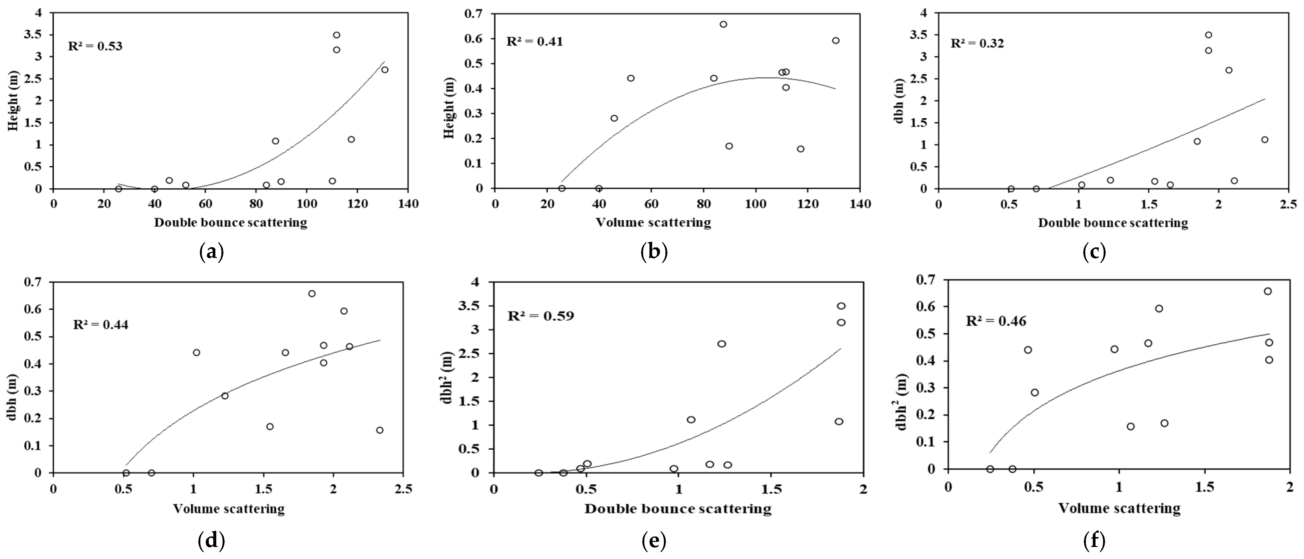
3.3.2. Regression Analysis with Polarimetric Parameters

The polarimetric parameters used in this study were CSI, RANSAC shape detection, VSI, BMI, cross-pol HH/HV ratio, co-pol HH/VV ratio, cross-pol VV/VH ratio and, RVI. The R2 value obtained for the CSI and biomass was 0.85, which showed a higher correlation between the canopy and the biomass. The ecosystem comprises more vertical and woody structures. The correlation R2 obtained between VSI and biomass was 0.49, which clearly showed that the thickness of the canopy was less; hence, VSI is less significant in the biomass assessment [30]. The R2 value obtained for BMI and biomass was 0.58 and 0.59 for RVI and biomass. This emphasizes the greater significance of RVI over BMI.

3.3.3. Regression Analysis with Backscatter and Textural Parameters

The biomass correlation was carried out using 7 textural variables, namely, mean, entropy, correlation, homogeneity, second moment (ASM), contrast, and variance. The backscatter values for HH and HV intensity were also considered. The regression analysis showed both a negative and a positive correlation. This is because in the modeling, both positive and negative correlations were useful in regulating the significance of the independent variables over the dependent variables. As can be seen in Figure 8, the positive R2 value was obtained with entropy and variance. The R2 value for the entropy was 0.21. The R2 value obtained for the variance and biomass was 0.52. The degree of randomness and variability of the area was more relevant, whereas the negative R2 value obtained was for ASM and mean. Therefore, textural parameters such as ASM, entropy, variance, and mean were significant in predicting the biomass of a natural forest.
The relation between the backscatter values for HH and HV intensity and the biomass showed that the R2 value obtained for HH intensity and biomass was 0.40, while 0.49 was obtained for HV intensity. Log transformation was then conducted to enhance the correlation between the variables HH and HV intensity with the biomass. Thus, the R2 value increased to 0.67 and 0.77 for HH and HV intensity with the biomass, respectively.

3.3.4. Regression between ALOS PALSAR L-Band and TLS-Derived Variables

The double-bounce and volume scattering were regressed with the height obtained using point cloud. The double-bounce scattering component was found to be more significant. As can be seen in Figure 9, the relation was not linear. The regression between height and volume scattering was log-transformed to better fit with an R2 value of 0.40, while the double-bounce and height were transformed to a higher order to obtain a better correlation with the R2 value of 0.53.
The double-bounce scattering component showed a correlation of 0.32 with dbh, which was a high-order relation, while dbh and volume scattering were log-transformed, yielding an R2 value of 0.44. A linear relation was found between dbh2, double-bounce, and the volume-scattering components. The correlation value was enhanced to 0.59 with the high-order polynomial relation for dbh2 and double-bounce, while the dbh2 and volume scattering were log transformed to show some relation, yielding an R2 value of 0.46. Here, the double-bounce showed a better correlation with dbh2.

3.3.5. Integration of Outputs of ALOS PALSAR and TLS

RF Regression Approach

Based on the correlation values of the 19 variables, the RF regression approach was used to integrate the TLS and SAR parameters. The % IncMSE showed the mean square error in the absence of any independent variables, while the IncNodePurity defined the purity of nodes at ntree in the presence of any important variables, as shown in Figure 10a.
In Figure 10c, the range of error is shown as per the number of trees. As the number of trees increased, the error of the graph decreased. Training datasets and RMSE were used to optimize the parameter (ntree, mtry) values and found values that were used for the best prediction of the dependent variable (AGB). In Figure 10d, the prediction and observed biomass values were plotted based on the best RMSE and R2 values, which were 38.95 and 0.94, respectively. Parameters such as ntree and mtry were optimized repeatedly to obtain the best results and reduce errors.
A graph between the RMSE and the number of variables was plotted to obtain the cross-validation of the number of variables taken for the estimation of the dependent variable. The forest error rate was calculated using Out-of-Bag (OOB) error analysis. OOB error was calculated for four mtry values. The mtry value for which OOB fewer errors were found was 4, while the highest probability of error was found for mtry 16. Using this method, each tree was tested on 1/3rd of the number of observations and not used in building the tree, indicating that the high strength of the tree showed a lower error. The maximum error obtained for mtry was 16 due to the high correlation between trees. The lowest error was obtained for mtry 4 due to the lesser correlation between the trees.

ANN Regression Approach

ANN were trained and tested with 23 independent variables. The variables were divided based on the number of weights assigned to each variable. The hidden layers were optimized to obtain a better R2 and RMSE. The negative weight assigned to any variable indicated the least contribution of that variable. The predicted and observed values of biomass are shown in Figure 11. The R2 value obtained for the ANN was 0.77. The number of hidden layers was fitted to ensure maximum accuracy for the prediction. Several hidden layers were tried to ensure minimum RMSE and maximum accuracy for the model. Figure 3 shows the different number of hidden layers and their accuracy at each level. Based on the R2 and RMSE of the model, an analysis was conducted and spatial distribution of biomass was carried out. The R2 value for RF was 0.94, the RMSE was 59.72 ton ha−1, and the percentage RMSE was 15.97. The R2 value of ANN was 0.77, with an RMSE of 98.46 ton ha−1 and a percentage RMSE of 26.32, as shown in Table 1. Based on this analysis, the RF was found to be the best model for predicting biomass.

Spatial Distribution and Uncertainty of Biomass

The spatial distribution of biomass was conducted with RF predictions over the region of the Barkot Forest Range. The variable used for the spatial distribution encompassed the ALOS PALSAR GLCM textural variables as well as the polarimetric and TLS-derived parameters. The predicted biomass range was between 122.46 and 581.89 ton ha−1.
The uncertainty distribution of AGB over the Barkot Forest Range was conducted using the bootstrap resampling method and the Monte Carlo approach. The uncertainty ranged from 15.75 to 85.14 ton ha−1. The percentage of uncertainty obtained was 20.54%. The uncertainty map of the AGB and biomass spatial distribution is shown in Figure 12.

4. Discussion

In this study, we used terrestrial LiDAR (TLS) and ALOS PALSAR L-band derived variables to address the biomass saturation problem in forest regions. This method can be applied mainly in temperate forest zones, but can also be used in other forest-type regions. The RF and ANN model training was carried out using the calibration data. Previous research has shown that biomass value improvisation can be achieved by integrating different datasets or parameters derived from satellite data [19].
It has been shown that machine learning algorithms such as RF and ANN can estimate AGB with considerable accuracy. Overall, the RF showed promising accuracy when integrated with different RS (Remote Sensing) datasets over linear regression modeling [31].
The use of integrated data has shown great promise in reducing the underestimation of forest biomass values. Using a single RS dataset to predict biomass can result in considerable uncertainty [32]. SAR data can be used to estimate biomass, but there is a problem with the saturation of specific bands as forest density increases [33]. It has been observed that LiDAR data are more reliable in estimating biomass because they maintain the precision and accuracy of the predicted biomass. These data have yielded promising results, with an R2 value of 0.98 and an RMSE of 0.08 Mg [34]. The collective information obtained from both SAR and LiDAR is key in overcoming the biomass saturation problem in SAR when using machine learning. This is because several machine learning algorithms have already been proven to yield the best results in estimating forest biomass.
The ALOS PALSAR-derived variables showed an important correlation with biomass. The GLCM texture variables showed a potential correlation with biomass, improving the area’s biomass prediction values. In one study, it was shown that textural information yields good correlation with biomass, improving the AGB estimation [35]. ALOS PALSAR polarimetric parameters and Yamaguchi decomposition parameters, such as surface scattering, double-bounce, and volume scattering, were used to establish a correlation with the biomass. The results revealed that the CSI, RVI, and BMI showed a potentially high correlation with biomass [36].
The uncertainty prediction was also performed for the RF model since the quantification of uncertainty was required to prove the model’s performance. The uncertainty in the spatially distributed AGB indicated that the pattern of forest distribution plays a crucial role in modeling biomass. Moreover, the uncertainty value was lower in the high-density areas of the forest and higher in the low-density areas because of the low correlation of biomass with tree attributes derived using ALOS.

5. Conclusions

In the current research, biomass was predicted using both ALOS PALSAR L-band and TLS-derived parameters in the study area of the Barkot Forest Range. Biomass was calculated using TLS-derived parameters. Correlations were also examined between biomass and various SAR parameters, such as texture (GCLM co-occurrence), backscattered values, polarimetric ratios, other SAR indices, and parameters derived using TLS. Thus, the two models, RF and ANN, were trained with field data. Then, the integration of the above-mentioned parameters or indices was conducted using two machine learning algorithms, RF and ANN. The best fit model obtained for the prediction of biomass was RF, with an R2 value of 0.94 and an RMSE of 15.9%. In contrast, the R2 obtained for ANN was 0.77, with an RMSE of 26.3%. It has been concluded that L-band integration with TLS-derived parameters shows great potential for the assessment of forest areas with very high biomass. The uncertainty can be mitigated using different machine learning algorithms and increasing the number of variables to train the model.

Author Contributions

Methodology, conceptualization, data analysis, writing, result interpretation: A.S. (Arunima Singh); Writing: S.K.P.K.; conceptualization, methodology: S.N.; writing—review and editing: H.P.; uncertainty analysis of results: S.G., A.S. (Ankur Srivastava) and N.K. helped in APC for the publication. All authors have read and agreed to the published version of the manuscript.

Funding

The research was not funded by any external sources. Only APC was provided by A.S. (Ankur Srivastava).

Data Availability Statement

Not applicable.

Acknowledgments

This research was undertaken as part of an M. Tech. dissertation for A.S. at the Indian Institute of Remote Sensing (IIRS), Dehradun, India. The authors also thank the Director and the Dean Academics of the IIRS for their continuous support and guidance. A.S. would like to acknowledge the late P. K. Champati ray for his valuable guidance. Uttarakhand Forest Department’s support in the field data collection is duly acknowledged.

Conflicts of Interest

The authors declare no conflict of interest.

References

  1. Houghton, R.A.; Hall, F.; Goetz, S.J. Importance of biomass in the global carbon cycle. J. Geophys. Res. Biogeosci. 2009, 114, G00E03. [Google Scholar] [CrossRef]
  2. Brede, B.; Calders, K.; Lau, A.; Raumonen, P.; Bartholomeus, H.M.; Herold, M.; Kooistra, L. Non-destructive tree volume estimation through quantitative structure modelling: Comparing UAV laser scanning with terrestrial LIDAR. Remote Sens. Environ. 2019, 233, 111355. [Google Scholar] [CrossRef]
  3. Silva, C.A.; Duncanson, L.; Hancock, S.; Neuenschwander, A.; Thomas, N.; Hofton, M.; Fatoyinbo, L.; Simard, M.; Marshak, C.Z.; Armston, J.; et al. Fusing simulated GEDI, ICESat-2 and NISAR data for regional aboveground biomass mapping. Remote Sens. Environ. 2021, 253, 112234. [Google Scholar] [CrossRef]
  4. Kattenborn, T.; Leitloff, J.; Schiefer, F.; Hinz, S. Review on Convolutional Neural Networks (CNN) in vegetation remote sensing. ISPRS J. Photogramm. Remote Sens. 2021, 173, 24–49. [Google Scholar] [CrossRef]
  5. Mangla, R.; Kumar, S.; Nandy, S. Random forest regression modelling for forest aboveground biomass estimation using RISAT-1 PolSAR and terrestrial LiDAR data. In Proceedings of the Lidar Remote Sensing for Environmental Monitoring XV, New Delhi, India, 4–7 April 2016; Singh, U.N., Sugimoto, N., Jayaraman, A., Seshasai, M.V.R., Eds.; SPIE: Bellingham, WA, USA, 2016; Volume 9879, p. 98790Q. [Google Scholar]
  6. Ho Tong Minh, D.; Ndikumana, E.; Vieilledent, G.; McKey, D.; Baghdadi, N. Potential value of combining ALOS PALSAR and Landsat-derived tree cover data for forest biomass retrieval in Madagascar. Remote Sens. Environ. 2018, 213, 206–214. [Google Scholar] [CrossRef]
  7. Leonardo, E.M.C.; Watt, M.S.; Pearse, G.D.; Dash, J.P.; Persson, H.J. Comparison of TanDEM-X InSAR data and high-density ALS for the prediction of forest inventory attributes in plantation forests with steep terrain. Remote Sens. Environ. 2020, 246, 111833. [Google Scholar] [CrossRef]
  8. Montesano, P.M.; Nelson, R.F.; Dubayah, R.O.; Sun, G.; Cook, B.D.; Ranson, K.J.R.; Næsset, E.; Kharuk, V. The uncertainty of biomass estimates from LiDAR and SAR across a boreal forest structure gradient. Remote Sens. Environ. 2014, 154, 398–407. [Google Scholar] [CrossRef]
  9. Peregon, A.; Yamagata, Y. The use of ALOS/PALSAR backscatter to estimate above-ground forest biomass: A case study in Western Siberia. Remote Sens. Environ. 2013, 137, 139–146. [Google Scholar] [CrossRef]
  10. Santoro, M.; Wegmüller, U.; Askne, J. Forest stem volume estimation using C-band interferometric SAR coherence data of the ERS-1 mission 3-days repeat-interval phase. Remote Sens. Environ. 2018, 216, 684–696. [Google Scholar] [CrossRef]
  11. Kushwaha, S.K.P.; Singh, A.; Jain, K.; Mokros, M. Optimum Number and Positions of Terrestrial Laser Scanner to derive DTM at Forest plot level. Int. Arch. Photogramm. Remote Sens. Spat. Inf. Sci. 2022, XLIII-B3-2, 457–462. [Google Scholar] [CrossRef]
  12. Liang, X.; Hyyppä, J.; Kaartinen, H.; Lehtomäki, M.; Pyörälä, J.; Pfeifer, N.; Holopainen, M.; Brolly, G.; Francesco, P.; Hackenberg, J.; et al. International benchmarking of terrestrial laser scanning approaches for forest inventories. ISPRS J. Photogramm. Remote Sens. 2018, 144, 137–179. [Google Scholar] [CrossRef]
  13. Thapa, R.B.; Watanabe, M.; Motohka, T.; Shimada, M. Potential of high-resolution ALOS-PALSAR mosaic texture for aboveground forest carbon tracking in tropical region. Remote Sens. Environ. 2015, 160, 122–133. [Google Scholar] [CrossRef]
  14. Santoro, M.; Cartus, O.; Fransson, J.E.S. Integration of allometric equations in the water cloud model towards an improved retrieval of forest stem volume with L-band SAR data in Sweden. Remote Sens. Environ. 2021, 253, 112235. [Google Scholar] [CrossRef]
  15. Stovall, A.E.L.; Shugart, H.H. Improved biomass calibration and validation with terrestrial lidar: Implications for future LiDAR and SAR missions. IEEE J. Sel. Top. Appl. Earth Obs. Remote Sens. 2018, 11, 3527–3537. [Google Scholar] [CrossRef]
  16. Gleason, C.J.; Im, J. Forest biomass estimation from airborne LiDAR data using machine learning approaches. Remote Sens. Environ. 2012, 125, 80–91. [Google Scholar] [CrossRef]
  17. Mutanga, O.; Adam, E.; Cho, M.A. High density biomass estimation for wetland vegetation using worldview-2 imagery and random forest regression algorithm. Int. J. Appl. Earth Obs. Geoinf. 2012, 18, 399–406. [Google Scholar] [CrossRef]
  18. Powell, S.L.; Cohen, W.B.; Healey, S.P.; Kennedy, R.E.; Moisen, G.G.; Pierce, K.B.; Ohmann, J.L. Quantification of live aboveground forest biomass dynamics with Landsat time-series and field inventory data: A comparison of empirical modeling approaches. Remote Sens. Environ. 2010, 114, 1053–1068. [Google Scholar] [CrossRef]
  19. Dang, A.T.N.; Nandy, S.; Srinet, R.; Luong, N.V.; Ghosh, S.; Senthil Kumar, A. Forest aboveground biomass estimation using machine learning regression algorithm in Yok Don National Park, Vietnam. Ecol. Inform. 2019, 50, 24–32. [Google Scholar] [CrossRef]
  20. Foody, G.M.; Boyd, D.S.; Cutler, M.E.J. Predictive relations of tropical forest biomass from Landsat TM data and their transferability between regions. Remote Sens. Environ. 2003, 85, 463–474. [Google Scholar] [CrossRef]
  21. Mukesh; Manhas, R.K.; Tripathi, A.K.; Raina, A.K.; Gupta, M.K.; Kamboj, S.K. Sand and clay mineralogy of sal forest soils of the Doon Siwalik Himalayas. J. Earth Syst. Sci. 2011, 120, 123–144. [Google Scholar] [CrossRef] [Green Version]
  22. Watham, T.; Patel, N.R.; Kushwaha, S.P.S.; Dadhwal, V.K.; Kumar, A.S. Evaluation of remote-sensing-based models of gross primary productivity over Indian sal forest using flux tower and MODIS satellite data. Int. J. Remote Sens. 2017, 38, 5069–5090. [Google Scholar] [CrossRef]
  23. Singh, A.; Kushwaha, S.K.P.; Nandy, S.; Padalia, H. An approach for tree volume estimation using RANSAC and RHT algorithms from TLS dataset. Appl. Geomat. 2022, 14, 785–794. [Google Scholar] [CrossRef]
  24. Singh, A.; Kushwaha, S.K.P.; Nandy, S.; Padalia, H. Novel Approach for Forest allometric eqaution modelling with RANSAC shape detection using Terrestrial Laser Scanner. Int. Arch. Photogramm. Remote Sens. Spat. Inf. Sci. 2022, XLVIII-4/W, 133–138. [Google Scholar] [CrossRef]
  25. Olofsson, K.; Holmgren, J.; Olsson, H. Tree stem and height measurements using terrestrial laser scanning and the RANSAC algorithm. Remote Sens. 2014, 6, 4323–4344. [Google Scholar] [CrossRef] [Green Version]
  26. Rosich, B.; Meadows, P.J.; Monti-Guarnieri, A. ENVISAT ASAR Product Calibration and Product Quality Status. 2004. Available online: https://www.researchgate.net/publication/246078768_ENVISAT_ASAR_Product_Calibration_and_Product_Quality_Status (accessed on 19 December 2022).
  27. Bergervoet, J.R.; van Campen, P.C.; van der Sanden, W.A.; de Swart, J.J. Phase shift analysis of 0–30 MeV pp scattering data. Phys. Rev. C 1988, 38, 15–50. [Google Scholar] [CrossRef] [Green Version]
  28. Yamaguchi, Y.; Moriyama, T.; Ishido, M.; Yamada, H. Four-component scattering model for polarimetric SAR image decomposition. IEEE Trans. Geosci. Remote Sens. 2005, 43, 1699–1706. [Google Scholar] [CrossRef]
  29. Haralick, R.M.; Dinstein, I.; Shanmugam, K. Textural Features for Image Classification. IEEE Trans. Syst. Man Cybern. 1973, SMC-3, 610–621. [Google Scholar] [CrossRef] [Green Version]
  30. Pope, K.O.; Rey-Benayas, J.M.; Paris, J.F. Radar remote sensing of forest and wetland ecosystems in the Central American tropics. Remote Sens. Environ. 1994, 48, 205–219. [Google Scholar] [CrossRef]
  31. Dube, T.; Mutanga, O. Evaluating the utility of the medium-spatial resolution Landsat 8 multispectral sensor in quantifying aboveground biomass in uMgeni catchment, South Africa. ISPRS J. Photogramm. Remote Sens. 2015, 101, 36–46. [Google Scholar] [CrossRef]
  32. Zhao, P.; Lu, D.; Wang, G.; Liu, L.; Li, D.; Zhu, J.; Yu, S. Forest aboveground biomass estimation in Zhejiang Province using the integration of Landsat TM and ALOS PALSAR data. Int. J. Appl. Earth Obs. Geoinf. 2016, 53, 1–15. [Google Scholar] [CrossRef]
  33. Bouvet, A.; Mermoz, S.; Le Toan, T.; Villard, L.; Mathieu, R.; Naidoo, L.; Asner, G.P. An above-ground biomass map of African savannahs and woodlands at 25 m resolution derived from ALOS PALSAR. Remote Sens. Environ. 2018, 206, 156–173. [Google Scholar] [CrossRef]
  34. Beyene, S.M.; Hussin, Y.A.; Kloosterman, H.E.; Ismail, M.H. Forest Inventory and Aboveground Biomass Estimation with Terrestrial LiDAR in the Tropical Forest of Malaysia. Can. J. Remote Sens. 2020, 46, 130–145. [Google Scholar] [CrossRef]
  35. Liao, Z.; He, B.; Quan, X. Potential of texture from SAR tomographic images for forest aboveground biomass estimation. Int. J. Appl. Earth Obs. Geoinf. 2020, 88, 102049. [Google Scholar] [CrossRef]
  36. Chowdhury, T.; Thiel, C.; Schmullius, C.; Stelmaszczuk-Górska, M. Polarimetric Parameters for Growing Stock Volume Estimation Using ALOS PALSAR L-Band Data over Siberian Forests. Remote Sens. 2013, 5, 5725–5756. [Google Scholar] [CrossRef] [Green Version]
Figure 1. Study area [23].
Remotesensing 15 01143 g001
Figure 2. Sampling location of the field data collection.
Remotesensing 15 01143 g002
Figure 3. Representation of (a) scheme of the plot scanned with TLS and retro-reflectors; (b) scanned plot with the location of reflectors (red dot); (c) extracted plot and single tree; and (d) trunk of the tree with noise, and after the application of a noise filter [23].
Remotesensing 15 01143 g003
Figure 4. Workflow of (a) RF approach and (b) ANN approach for biomass prediction.
Remotesensing 15 01143 g004
Figure 5. Methodology flowchart.
Remotesensing 15 01143 g005
Figure 6. Correlation plots between TLS-derived parameters and biomass. (a) Correlation between height and biomass; (b) log-transformed correlation between height and biomass; (c) correlation between dbh and biomass; and (d) correlation between dbh2 and biomass.
Remotesensing 15 01143 g006
Figure 7. Yamaguchi decomposition of ALOS PALSAR L-band data.
Remotesensing 15 01143 g007
Figure 8. (ag) Correlation between different SAR variables and the field-measured biomass.
Remotesensing 15 01143 g008
Figure 9. (af) Correlation plots of the ALOS PALSAR and TLS-derived variables.
Remotesensing 15 01143 g009
Figure 10. Visualization of (a) % IncMSE and IncNodePurity of the variables used to train the model; (b) out-of-bag (OOB) error while training the data; (c) estimated error based on different no. of trees, (d) error and RMSE of the number of variables and trees in the RF model; and (e) scatterplot for the observed and predicted biomass value (ton/ha).
Remotesensing 15 01143 g010aRemotesensing 15 01143 g010b
Figure 11. Scatterplot of the predicted Vs observed biomass (ton/ha) based on the ANN model.
Remotesensing 15 01143 g011
Figure 12. Visualization of the (a) spatial distribution of AGB (t/ha) and (b) uncertainty of AGB (t/ha).
Remotesensing 15 01143 g012
Table 1. Statistical parameters for the models.
Sr. No.ModelR2RMSE (ton ha−1)RMSE%RMSECV
1RF0.9459.7215.970.15
2ANN0.7798.4626.320.23
Disclaimer/Publisher’s Note: The statements, opinions and data contained in all publications are solely those of the individual author(s) and contributor(s) and not of MDPI and/or the editor(s). MDPI and/or the editor(s) disclaim responsibility for any injury to people or property resulting from any ideas, methods, instructions or products referred to in the content.

