Article

Superpixel Generation for Polarimetric SAR Images with Adaptive Size Estimation and Determinant Ratio Test Distance

1
College of Electronic Science and Technology, National University of Defense Technology, Changsha 410073, China
2
College of Information and Navigation, Air Force Engineering University, Xi’an 710077, China
*
Author to whom correspondence should be addressed.
Remote Sens. 2023, 15(4), 1123; https://doi.org/10.3390/rs15041123
Submission received: 17 November 2022 / Revised: 3 February 2023 / Accepted: 16 February 2023 / Published: 18 February 2023
(This article belongs to the Section Remote Sensing Image Processing)

Abstract

:
Superpixel generation of polarimetric synthetic aperture radar (PolSAR) images is widely used for intelligent interpretation due to its feasibility and efficiency. However, the initial superpixel size setting is commonly neglected, and empirical values are utilized. When prior information is missing, a smaller value will increase the computational burden, while a higher value may result in inferior boundary adherence. Additionally, existing similarity metrics are time-consuming and cannot achieve better segmentation results. To address these issues, a novel strategy is proposed in this article for the first time to construct the function relationship between the initial superpixel size (number of pixels contained in the initial superpixel) and the structural complexity of PolSAR images; additionally, the determinant ratio test (DRT) distance, which is exactly a second form of Wilks’ lambda distribution, is adopted for local clustering to achieve a lower computational burden and competitive accuracy for superpixel generation. Moreover, a hexagonal distribution is exploited to initialize the PolSAR image based on the estimated initial superpixel size, which can further reduce the complexity of locating pixels for relabeling. Extensive experiments conducted on five real-world data sets demonstrate the reliability and generalization of adaptive size estimation, and the proposed superpixel generation method exhibits higher computational efficiency and better-preserved details in heterogeneous regions compared to six other state-of-the-art approaches.

1. Introduction

Synthetic aperture radar (SAR) is less sensitive to atmospheric and illumination conditions [1,2]. Polarimetric SAR (PolSAR) can acquire more scattering information than SAR and has been widely used in many military and civilian fields [3,4]. Superpixel generation is an efficient step in PolSAR images’ automatic interpretation [5,6]. The term superpixel is a series of pixels with similar low-level characteristics and adjacent positions, which are similar to huge pixels [7,8]. With the development of imaging techniques, the high number of pixels in high-resolution PolSAR images brings significant challenges to the computational complexity of many algorithms. Moreover, the speckle noise of PolSAR images raises some difficulties in image interpretation. The crucial advantages of PolSAR images’ superpixel generation are a decrease in the impact of speckle noise and the calculation amount for subsequent interpretation [9,10]. Therefore, for the intelligent interpretation of PolSAR images, superpixel generation is urgently needed and widely studied [11,12].
There are roughly five existing categories of superpixel generation algorithms for PolSAR images, including density-based methods [13], graph-based methods [14,15], contour evolution methods [16,17], energy optimization methods [18] and clustering-based methods [8,19]. However, some methods such as graph-based methods [20,21] and energy optimization methods need to combine a variety of technical elements, such as the revised Wishart distance (RWD), edge map, and energy-driven sampling (SEEDS), to improve the accuracy, which is computationally demanding. The loss of the control aimed at the number of superpixels makes the application of density-based methods limited [22,23]. However, clustering-based methods are capable of generating controllable numbers of superpixels, regular shapes, and compact regions, which are popularly used as the preprocessing step of PolSAR image interpretation. Most clustering-based methods use the principle of the k-means algorithm [8], and some efficient similarity measurements are adopted for relabeling, such as the spatial distance and statistic distance.
Superpixel generation is a preprocessing step of PolSAR image interpretation; therefore, the indispensable abilities are higher accuracy and lower computational burden. Among the numerous superpixel generation methods, there are many methods that need to set some parameters, and one of the more important parameters is the initial superpixel block size or the number of initial superpixels (which can be converted into each other). This issue has not received much attention because most researchers use empirical values or ergodic parameter values. Moreover, some methods commonly sacrifice calculation time in exchange for the guarantee of boundary adherence. In other words, in the face of complex PolSAR images, smaller initial superpixel blocks are commonly used to ensure segmentation accuracy. Therefore, defining the value of the initial superpixel size is a challenging dilemma; that is, converting a qualitative problem into a quantitative problem.
Hu et al. [24] proposed an initialization method based on edge information to adaptively generate initial superpixel blocks based on SAR images. The edge information is introduced into the initialization step of the clustering center, which is divided into N L equal parts according to the preset N L at the edge and initialized according to the initial grid width at the non-edge; thus, the adaptive initial width is obtained. However, this method needs to set the initial grid width, and there is still a big difference between SAR data sets and PolSAR data sets. On the one hand, it is obvious that there is no universal solution to this issue. On the other hand, this is because the problem is difficult to define.
Therefore, from the point of view of how to better strike a balance between accuracy and efficiency, this paper innovatively proposes adopting the structural complexity of PolSAR images to estimate the adaptive initial superpixel size; that is, the adaptive number of pixels contained in the initial superpixel (marked as N a ). One of the significant features of the social and natural sciences is the complexity of patterns, which are objects’ essential properties. Bagrov et al. [25] proposed a universal method for calculating the structural complexity, including two-dimensional and three-dimensional patterns, which can be generalized to more classes. Inspired by this, we propose calculating the structural complexity of PolSAR images via Pauli decomposition. Importantly, the value of N a should be as large as possible while meeting an accuracy that enhances the computational efficiency. Clearly, a larger N a will reduce the computational burden of superpixel generation.
Clustering-based methods are widely used because of their irreplaceable superiority, such as simple linear iterative clustering (SLIC), linear spectral clustering (LSC), and iterative edge refinement (IER). The Wishart distance was adopted to obtain compact superpixels in 2014 [26]. Qin et al. [27] utilized the revised Wishart distance (RWD) with the SLIC method (POL-SLIC method). To decrease the amount of time consumed, Zhang et al. [28] adopted the fast calculation of the RWD with an IER framework [29]. Subsequently, we improved the above method through an innovative initialization method that initializes the input image with a hexagonal distribution, which is called HAWS [30]. The geodesic distance (GD), which measures the shortest distance between two real symmetric Kennaugh matrices, is also proposed to reduce the time cost of superpixel generation for PolSAR images [31]. However, the boundary adherence ability of the GD is slightly inferior to that of RWD. Akbari et al. [32] proposed the complex-kind Hotelling–-Lawley trace (HLT) to measure the similarity between pixels for improving the performance of PolSAR image change detection. Then, Yin et al. [10] introduced the HLT distance to boost the ability of POL-SLIC for PolSAR images. However, the computational burden is large because of the double calculations of the HLT distance to eliminate the nonsymmetric effect.
The adopted distance measurements of the above-mentioned algorithms are unsatisfactory due to the heavy computation with complex matrices. The GD can reduce the computational burden; however, some edges of generated superpixels are blurred. Therefore, a comprehensive distance with good performance in terms of accuracy and efficiency is necessary to generate superpixels for PolSAR images. Specifically, the determinant ratio test (DRT) statistic is proposed for change detection in PolSAR images [33]. The DRT distance can measure the similarity between two covariance matrices, which are assumed to follow a scaled complex Wishart distribution. Moreover, the distribution of DRT distance is a second form of Wilks’ lambda distribution. Therefore, we improved the DRT distance to enhance the performance of superpixel generation for PolSAR images. Notably, the calculation of the DRT is much simpler than the above-mentioned distance measurements, and the result of the DRT distance is a scalar value.
To provide better performance for superpixel generation as a preprocessing step, we adopt the structural complexity of PolSAR images to estimate adaptive N a (i.e., CEN). Moreover, the DRT distance with a hexagonal distribution is utilized to enhance the performance of superpixels. The main contributions of this article are summarized as follows:
  • The adaptive size estimation of the initial superpixel via the structural complexity is proposed for PolSAR image superpixel generation for the first time.
  • The DRT distance, with superior similarity measurement ability and computational efficiency compared to other distance measurements for PolSAR images, is utilized to generate compact superpixels.
  • Extensive experiments conducted on five real-world PolSAR data sets effectively demonstrate that the proposed CEN can adaptively estimate N a . Our proposed method can provide better computational performance with higher boundary adherence than six competitive superpixel generation methods.
The remainder of this article is organized as follows. Section 2 introduces the efficient DRT distance. The proposed CEN method and superpixel generation framework is expressed in Section 3. Section 4 shows the experiments and comparisons with six state-of-the-art methods based on five real-world PolSAR data sets. The conclusion is given in Section 5.

2. Determinant Ratio Test Distance

Generally, scattering matrix S is commonly used to express each pixel of a PolSAR image, defined as follows [34]:
S = S H H S H V S V H S V V ,
according to the reciprocity medium, S H V = S V H .
It is assumed that S is a d-dimensional complex vector, which follows a circular complex Gaussian distribution S N d C ( 0 , Σ ) , with a zero-mean vector and a covariance matrix Σ . To decrease the impact of speckle noise, the calculation of polarimetric multilooking is defined as:
X = 1 L = 1 L S S H , L d ,
where L represents the number of looks, ( . ) H denotes the Hermitian operator, and S represents the S with different numbers of looks. X Ω + C d × d is the multilook polarimetric covariance matrix, which is a random matrix. Specifically, it is the positive definite complex Hermitian matrix. When L d , the unnormalized sample covariance matrix defined as Z = L X follows the nonsingular complex Wishart distribution denoted as Z W d C ( L , Σ ) [35]. Additionally, X follows a scaled complex Wishart distribution X s W d C ( L , Σ ) . The probability density function (pdf) of X is f X ( X ) = f Z ( L X ) J Z X , where the J Z X = L d 2 represents the Jacobian determinant of the transformation Z = L X [33]. The pdf of X is
f X ( X ) = L L d | X | L d Γ d ( L ) | Σ | L etr L Σ 1 X ,
where etr ( . ) = exp ( tr ( . ) ) is the exponential trace operator, | . | is the determinant operator, and Γ d ( L ) is the multivariate gamma function of the complex kind defined as
Γ d ( L ) = π d ( d 1 ) / 2 i = 0 d 1 Γ ( L i ) ,
where Γ ( L ) is the standard Euler gamma function.
Let X and Y be statistically independent Hermitian positive definite random d × d matrices that follow scaled complex Wishart distributions with different distribution parameters defined as:
X s W d C L x , Σ x and Y s W d C L y , Σ y .
According to the imaging characteristic of the PolSAR image, any two points i and j in the image can be represented by these two matrices X and Y . When the above conditions are satisfied, Bouhlel et al. [33] innovatively proposed that the determinant ratio statistic is defined by
τ DRT = L x X L y Y .
For details of the proof, please see [33]. DRT is used to measure the similarity between the two polarimetric covariance matrices X and Y for change detection by the hypotheses [33]. For the particular case where L x = L y = L , the DRT statistic becomes τ DRT Λ ( 2 L , d , L ) . Hence, to measure the distance of a pixel i and a class center j, the DRT distance is defined as follows:
d DRT ( i , j ) = X i Y j .
The DRT statistic is able to produce a scalar value and is nonnegative with higher computational efficiency. Moreover, since heavy complex operations can be efficiently avoided via the DRT statistic, it is obviously better than the often-used Wishart distance.

3. Materials and Methods

First, the function relationship between the PolSAR image’s structural complexity and the number of pixels contained in the initial superpixel is constructed, and the adaptive size of the initial superpixel is estimated by calculating the PolSAR image’s structural complexity. Second, the hexagonal distribution is adopted to initialize the input PolSAR image with the estimated size. Then, the efficient DRT distance is utilized for relabeling. Finally, postprocessing is performed to obtain the final superpixels. Figure 1 shows the flowchart of the proposed method.

3.1. PolSAR Image Structural Complexity

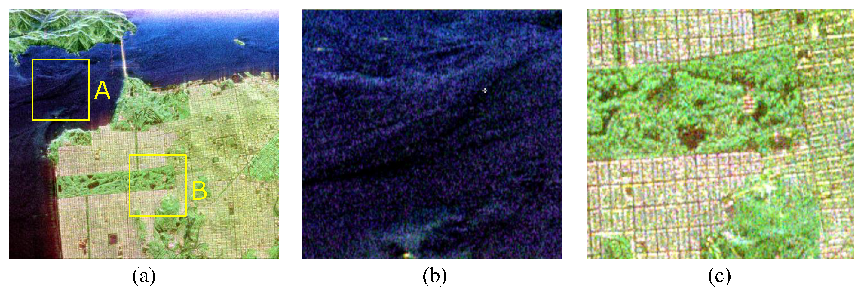
Complexity is difficult to precisely quantify. Figure 2a shows an AIRSAR L-Band PolSAR image from San Francisco Bay, United States. Regions A and B in Figure 2a are magnified to show the details in Figure 2b and Figure 2c, respectively. The terrain category of region A contains mainly water, while region B contains mainly buildings and vegetation. Clearly, according to visual analysis, the complexity of Figure 2c is higher than that of Figure 2b. However, quantifying the complexity is a difficult issue, and the complexity of Figure 2a, including regions A and B, is also troublesome. Bagrov et al. [25] proposed a method for calculating the structural complexity, including two-dimensional and three-dimensional models. Inspired by this, the above method is improved in this paper to calculate the structural complexity of a PolSAR image. The k P of the Pauli-basis scattering vector is given by
k P = S H H + S V V , S H H S V V , 2 S H V T S H H + S V V , S H H S V V , 2 S H V T 2 2 ,
where S H H + S V V , S H H S V V and S H V represent the three categories of terrain. For each pixel, we use blue, red, and green to represent their amplitudes | S H H + S V V | , | S H H S V V | , and | 2 S H V | , and obtain three color channels. The classified pseudo-color Pauli-RGB image can be obtained by mixing the three color channels.
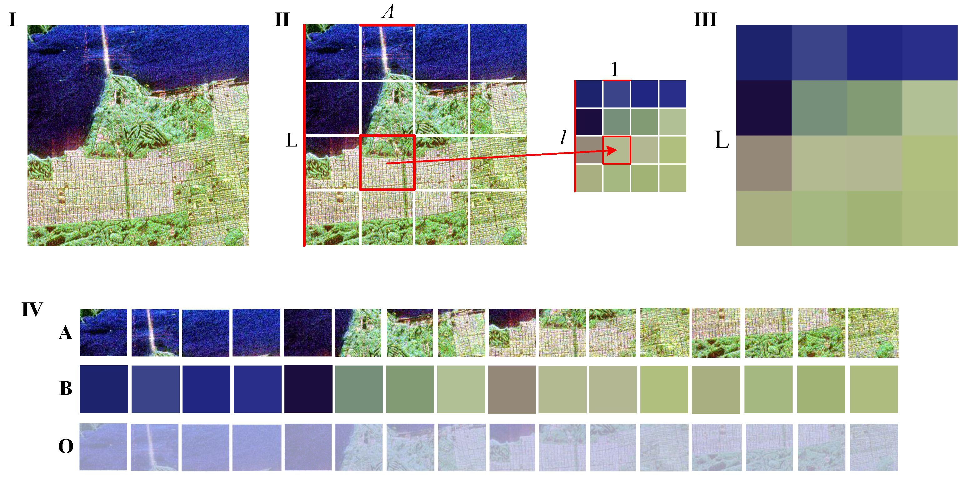
Specifically, a PolSAR image of 512 × 512 pixels as an example for calculating structural complexity is shown as Figure 3 [25]. Each pixel of a Pauli-RGB image can be represented by a vector s i j ; the i j denote the position of the pixel, which represents the scaled three color components in the RGB scheme with the range [ 1 , 1 ] . At each iteration of the coarse-graining procedure, the pattern is divided into blocks of Λ × Λ , and each block is substituted with a single pixel:
s i j ( k ) = 1 Λ 2 l m s Λ i + m , Λ j + l ( k 1 ) ,
where the l , m indices enumerate the pixels belonging to the same block and k is the number of iterations. This procedure is then repeated several times, resulting in a stack of renormalized patterns of different resolutions. An overlap of the pattern between scale k and k 1 is defined as:
O k , k 1 = 1 L k 1 2 i = 1 L k j = 1 L k s i j ( k ) · m = 1 Λ l = 1 Λ s Λ i + m , Λ j + l ( k 1 ) = Λ 2 L k 1 2 i = 1 L k j = 1 L k s i j 2 ( k ) = Λ 2 L k 1 2 · L k 2 · O k , k = O k , k ,
where k = 0 corresponds to the original pattern. The structural complexity C can be defined as an integral characteristic accounting for features emerging at every new scale shown by
C = k = 0 N 1 C k = k = 0 N 1 O k + 1 , k 1 2 O k , k + O k + 1 , k + 1 ,
where N is the total number of renormalization steps.

3.2. Estimation of the Adaptive Initial Superpixel Size

For clustering-based superpixel generation methods, the number of pixels contained in the initial superpixel block (marked as N ) is an essential parameter that basically determines the size of the final superpixel block. Generally, when other parameters remain constant, the smaller N is, the higher the precision is, but the longer the calculation time is. This is because most superpixel generation methods need to calculate the pairwise similarity, especially clustering-based methods, which need to constantly calculate the similarity between many pixels in multiple iterations. PolSAR images can obtain the rich polarimetric scattering information of targets. With the development of imaging platforms, extensive high-resolution PolSAR images need to be interpreted. Clearly, as an efficient preprocessing method for the intelligent interpretation of PolSAR images, superpixel generation methods should have high computational efficiency.
Generally, when more complex heterogeneous regions are segmented, a smaller N can adhere more closely to the edges of the real objects. Figure 4 and Figure 5 show examples of superpixel generation. According to Equation (11), the values of C are 0.293 and 0.267 for Figure 4a and Figure 5a, respectively. Clearly, the structural complexity of Figure 4a is larger than that of Figure 5a. Both the value of N = 64 and the smaller value of N = 36 can obtain superior edge adherence results in Figure 4b,c. However, the running time (RT) of N = 36 is longer than that of N = 64 . Similarly, for Figure 5a with a lower C , both the value of N = 64 and the larger value of N = 100 can generate compact superpixels in Figure 5b,c. The computational efficiency of N = 100 is obviously better than N = 64 . Nevertheless, quantifying a “small” or “large” N to obtain close superpixels and lighten the computational burden as much as possible remains a challenging issue.
When superpixel generation is based on terrain distribution or homogeneous or heterogeneous high-resolution PolSAR images, most researchers choose to adopt empirical values or traverse a certain range of parameter values to obtain the initial size. This method requires many computing resources, which reduces the significance of superpixel generation. More importantly, this method cannot meet the accuracy requirements when selecting a larger N to take into account the accuracy and computational efficiency of superpixel generation.
Clearly, Figure 4 and Figure 5 show a close relationship between the structural complexity and N for input PolSAR images. There is less manual processing in estimating the N using the structural complexity, which is entirely determined by the structural complexity of the input PolSAR image. Therefore, the estimated N a is an adaptive value according to the structural complexity of the input PolSAR image. This will greatly improve the computational efficiency of superpixel generation during preprocessing, make superpixel generation more convenient, and improve the utilization rate. Therefore, the functional relationship N a = f C between the structural complexity and N a should be constructed, and an appropriate value of N a can be calculated from the structural complexity C .
Generally, four criteria are adopted to quantitatively assess the results of superpixel generation, including boundary recall (BR), running time (RT), under-segmentation error (USE), and achievable segmentation accuracy (ASA) [8,36]. The BR is the ratio of boundary pixels shared by the obtained superpixels and the ground truth, and a higher BR value indicates that superpixel blocks agree better with the input image edges. The USE should be as low as possible for obtaining good superpixels.
The ASA is a performance upper-bound measure and the highest achievable accuracy of object segmentation. Undoubtedly, the higher the ASA value is, the higher the credibility of the segmentation result is, but it does not represent boundary adherence. To quantify the reasonableness of different values of N a , we propose the comprehensive accuracy, which is defined as
CA = BR + USE + ASA ,
where USE = 1 USE , USE 0 , 1 . Therefore, a larger value of USE represents a smaller USE , which means more reliable superpixels.
Different PolSAR data sets come from a variety of imaging platforms, and the interference in the imaging process is also distinct. In addition, the types of terrain distribution observed are unique, which makes different PolSAR data sets highly diverse. To make the constructed N a = f C have strong generalization ability and stability, this study utilizes polynomial curve fitting to construct the function relationship by collecting a large number of points C , N a . Polynomial curve fitting is usually used to optimize the square loss using the least squares method, and the idea is simple and easy to implement [37]. At the same time, the generated function is easy to utilize for estimating the adaptive N a in this paper.
There are few publicly available PolSAR data sets, and it is necessary to crop the existing PolSAR images to obtain large sample points C , N a . Evidently, the difference in C between each patch in the same image is quite disparate because of the various terrain categories in an individual image. When cropping a variety of PolSAR data sets, choosing the same step value will result in a large difference in C between patches, which will interfere with the accuracy and generalization ability of the polynomial curve fitting. Often, in the same image, when there is overlap between patches, the change in the C value may be continuous. Therefore, a strategy of pseudo-cropping is proposed to equalize the value of C . Details of obtaining sample points C , N a are summarized as follows:
(1)
Parameter initialization. Input a PolSAR image. Set values of the patch size, the presupposed difference between the patches C expdiff , and a predefined threshold G D i f f .
(2)
Pseudo-cropping. Crop the input PolSAR image to get n u m p c pseudo-patches with uniform steps. Calculate C p c = C p c _ 1 , , C p c _ n u m p c .
(3)
Real cropping. The total number of real-patches of the input PolSAR image is n u m r c = max C p c min C p c / C expdiff .
(4)
Calculate C r c . Obtain n u m r c real patches with uniform steps. Calculate C r c = { C r c _ 1 , , C r c _ n u m r c } .
(5)
Superpixel generation. Superpixel generation for patch r c _ i is r c _ 1 , , r c _ n u m r c ; let the input N traverse the range n u m s u p _ 1 , n u m s u p _ m . Record the CA r c _ s u p _ i of N = n u m s u p _ i of the patch r c _ i .
(6)
Calculate differences. Sort the CA r c _ s u p _ 1 , , CA r c _ s u p _ m from highest to lowest CA r c _ s u p _ s m , , CA r c _ s u p _ s 1 , and calculate the difference Diff r c _ s u p _ s 1 =   CA r c _ s u p _ s m CA r c _ s u p _ s i , where r c _ s u p _ s i r c _ s u p _ s m .
(7)
Calculate N a . Select the corresponding N r c _ s u p values of Diff r c _ s u p _ s i G Diff , and sort the corresponding N r c _ s u p _ p , , N r c _ s u p _ 1 from highest to lowest. Therefore, N a = N r c _ s u p _ p .
(8)
Calculate sample points C , N a . Repeat step (5) to step (7) to obtain N a _ 1 , , N a _ n u m r c of n u m r c patches for the input PolSAR image, and sample points { C r c _ 1 , N a _ 1 , ,   C r c _ n u m r c , N a _ n u m r c } .
A large number of sample points C , N a can be obtained based on the diverse PolSAR images with different patch sizes. Moreover, the flowchart of the proposed CEN is shown in Figure 6.

3.3. Superpixel Generation Based on the DRT Distance

First, the hexagonal distribution is adopted to initialize the input PolSAR image based on the N a via the CEN method. Then, the DRT distance is utilized for relabeling. Finally, postprocessing is performed to obtain the final superpixels.

3.3.1. Initialization

In an image, unstable pixels [28] are pixels whose labels are likely to change and should be checked in the next iteration. The definition of unstable pixels is as follows:
UP = p | n t p n t q   and n t q t q , q N b p ,
where p and q represent pixels in the image domain. N b ( p ) is the neighborhood function, and a 4-connected neighborhood is utilized in the experiments. Further, t ( i ) represents the label of i, n t ( i ) represents the new label after one iteration, and i = p , q .
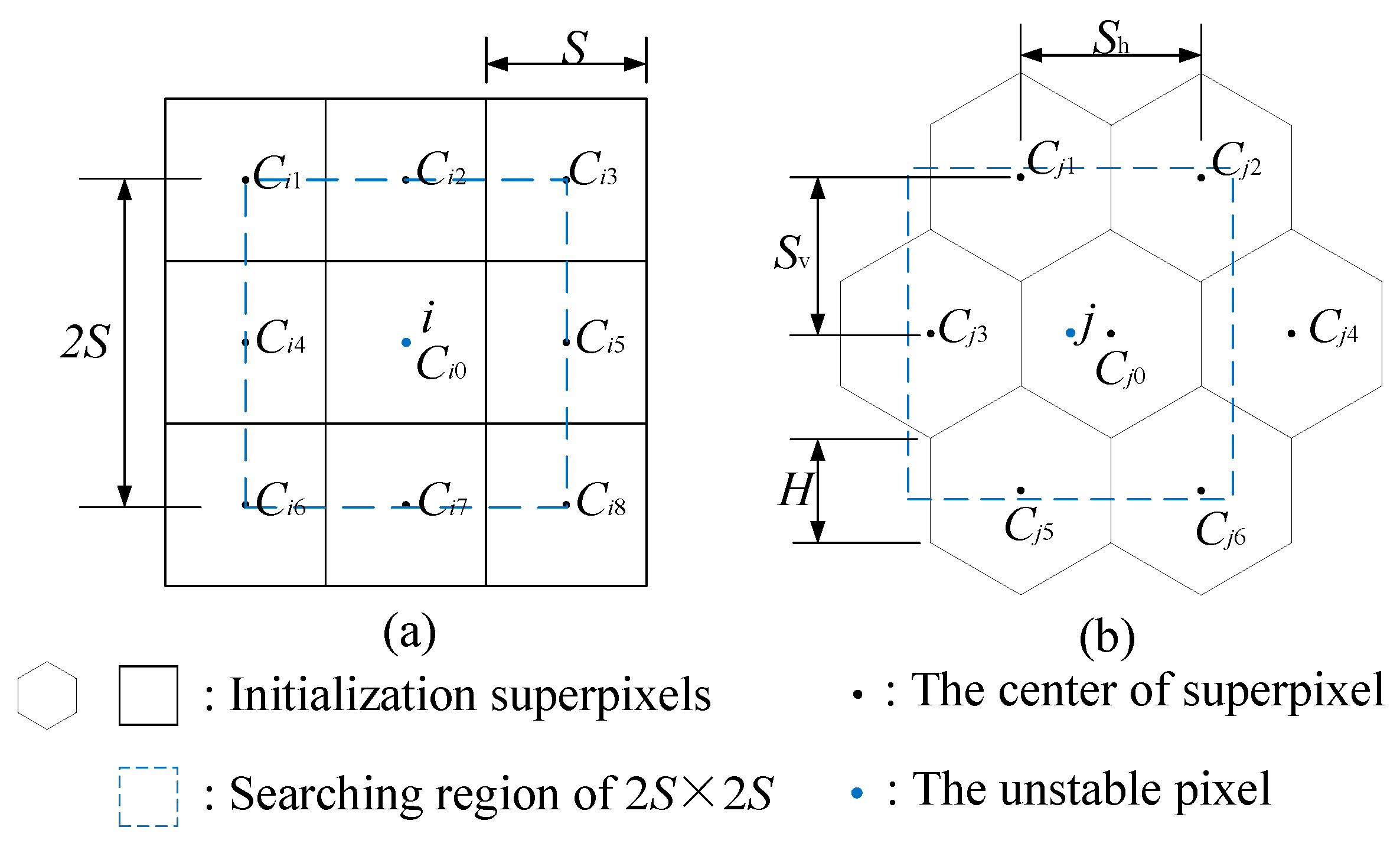
Figure 7 shows the square (grid) initialization and hexagonal initialization, and rectangles with black solid lines are initialized superpixels. Specifically, both square and hexagonal distributions’ searching region is 2 S × 2 S , where S = N a . In the local regions of the same size, the square distribution has nine clustering centers ( C i 0 C i 8 ); however, Figure 7b shows only six clustering centers ( C j 0 , C j 1 , C j 2 , C j 3 , C j 5 and C j 6 ) for the hexagonal distribution. Therefore, the hexagonal distribution can reduce the number of redundant calculations with just six distance calculations, compared with the square distribution of nine distance calculations [30], for one unstable pixel.

3.3.2. Local Relabeling and Postprocessing

The DRT and the spatial distance are utilized for relabeling [8], defined as follows:
D i , j = d DRT i , j m DRT 2 + d s i , j S 2 , d s i , j = x j x i 2 + y j y i 2 ,
where m DRT is the compactness parameter, d s i , j is the spatial distance, and S = N a .
A postprocessing procedure based on the DRT distance is adopted in this study [28]. When the size of a superpixel is smaller than N t h = N a / 4 , the dissimilarity between this superpixel R i and its eight neighboring superpixels R j will be calculated respectively, defined as follows:
G R i , R j = 1 q C i d i a g C j d i a g C i d i a g + C j d i a g 1 ,
where C d i a g is a vector consisting of the diagonal elements of the center C matrix of a superpixel, . 1 denotes the 1-norm of a matrix, and q is the dimension of k P . When G G t h , this superpixel is merged into the current neighbor. The predefined threshold G t h = 0.3 is adopted throughout this article [28]. The details of our proposed method are summarized as follows:
(1)
Initialization. Initialize the input PolSAR image as a hexagonal distribution by utilizing N a via the proposed CEN. Set the iteration index n = 0 .
(2)
Local relabeling. If n n m a x or the unstable pixel set is empty, then the algorithm ends and proceeds to (4). Otherwise, Equation (14) is adopted to relabel all unstable pixels with the 2 S × 2 S searching area.
(3)
Updating. Update the superpixel models and the unstable pixel set. Set n = n + 1 and return to (2).
(4)
Postprocessing. Locate the superpixels with sizes smaller than N t h and merge them with the predefined criterion.
Because the algorithm in this paper is initialized by a regular hexagon and the DRT distance uses high efficiency to measure the similarity between pixels for relabeling, taking into account the spatial continuity using the spatial distance, the algorithm proposed in this paper is called the HADS algorithm. Moreover, the flowchart of the proposed HADS is shown in Figure 6.

4. Results and Discussion

This section carries out experiments on five actual PolSAR data sets to discuss the effectiveness of the proposed CEN and HADS. In Section 4.1, we first introduce the details of five real-world PolSAR data sets. Section 4.2 introduces the details of polynomial curve fitting using numerous points C , N a in the proposed CEN method. In Section 4.3, the accuracy of the proposed CEN method is verified based on the five real-world PolSAR data sets. In Section 4.4 and Section 4.5, experiments and discussions about two actual PolSAR data sets are presented.

4.1. Data Sets

Figure 8 shows the five real-world data sets used in our experiments, and Table 1 presents the details of these data sets. Moreover, according to [34,38], the manual segmentation maps of the five real-world data sets are adopted for quantitative evaluation as ground truth. Data sets 1 and 2 were acquired over Flevoland, the Netherlands. Figure 8a,c shows that data sets 1 and 2 contain a large number of different categories of crops, including potatoes, fruit, and oats. Therefore, the edges of the real objects are more regular. In contrast, data set 3 is in San Francisco [34], CA, USA, and large regions of homogeneity can be clearly observed in Figure 8e, even though the boundary is blurred at some edges. The ESAR data set acquired over Oberpfaffenhofen, Germany, contains many complex heterogeneous regions and blurred boundaries. Data set 5, acquired over Changsha, Hunan Province, China, on 13 July 2017, is a C-band PolSAR image with 1000 × 1000 pixels, which is a Gaofen-3 (GF-3) data set and is adopted for the first time. Figure 8 shows that data set 5 mainly contains vegetation, urban buildings, and water. Changsha has many dense buildings; part of the vegetation is urban greening, so it is intertwined with buildings.
It can be observed that the five data sets adopted in this study come from different regional types, including many classical terrain categories, both large homogeneous regions and complex heterogeneous regions. Diversified real-world data sets are beneficial to the curve fitting of the proposed CEN and verification of accuracy.

4.2. Experimental Setup of the Proposed CEN

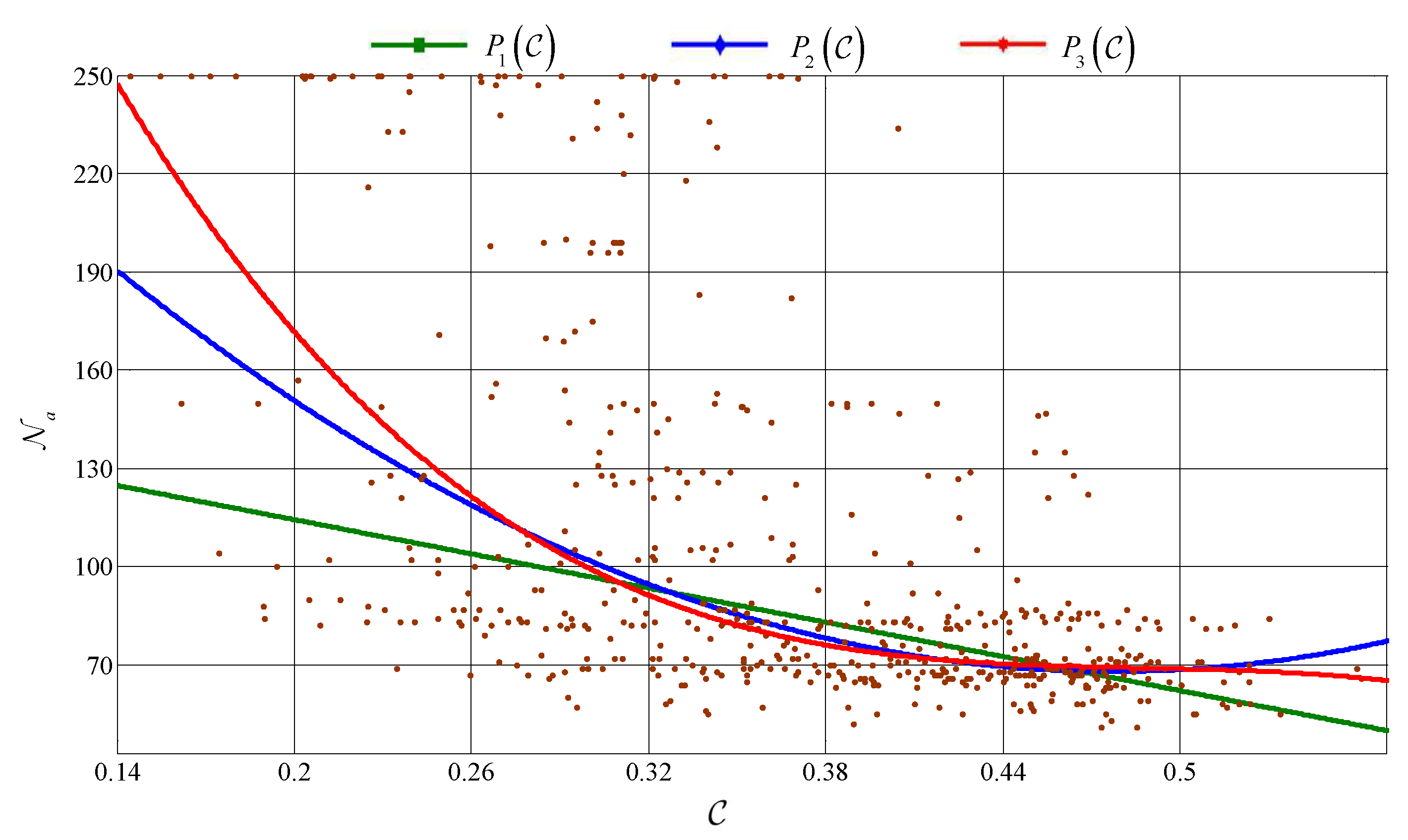
Considering the stability and generalization ability of the fitting function, data sets 1–4, including vegetation, buildings, crops, water, and other common terrain objects, are adopted to construct sample points to fit the generalized polynomial. The patch size is 512 × 512 and 256 × 256 . Clearly, a smaller patch size represents more focused attention, and Diff _ C p c = max C p c min C p c is larger. Table 2 shows the details of the image patches from data sets 1–4. Some examples of patches with different sizes are shown in Figure 9. The G D i f f = 0.2 for data sets 1–4 in this study. Therefore, we conducted 126,334 superpixel generations to obtain 559 sample points C , N a . Then, polynomial curve fitting was adopted to construct N a = P n C , as shown in Figure 10. The robust least-squares fitting method was adopted by minimizing the least absolute residuals in the polynomial curve fitting [37].
The three function expressions with different orders n are shown in Equation (16).
N a = P n C = 174.1 C + 149.1 , n = 1 1077 C 2 1028 C + 313.2 , n = 2 4113 C 3 + 6013 C 2 2948 C + 553.7 , n = 3
Compared with the optical images, the value of C is larger, which also confirms that the PolSAR images have the characteristics of speckle noise interference, many kinds of terrain objects, and complex distribution patterns. Only a small number of patches have a value of C less than 0.25, and 8% of the patches are mainly a single category of terrain, such as water with less noise in Figure 9. Therefore, the slope of the curve is very large when C < 0.25 ; at this time, the larger N a can still adhere to the edge of the real object well.
When C is approximately 0.4, the image usually contains more than two categories of terrain and the distribution is different, which is also a common complexity in PolSAR images. When C > 0.55 , the image commonly contains more detailed information, the edge is blurred, and there are large heterogeneous areas or the image is seriously disturbed by noise. To ensure the accuracy of superpixel generation, the value of N a is smaller. Specifically, Figure 9 shows the respective values of C . Obviously, P 3 C can describe the function relationship between C and N a more accurately than P 1 C and P 2 C in Figure 10.

4.3. Curve Effectiveness Evaluation

To validate the effectiveness of the curve fitted in this paper, this subsection utilizes data sets 1–5 to evaluate the estimation accuracy with the randomly generated patch sizes compared to those grid sizes in the polynomial curve fitting. Moreover, data set 5 and data sets 1–4 used in the polynomial curve fitting come from different sensors and have different terrain characteristics. These experimental settings have high requirements for the stability of the function shown in Equation (16). The evaluation details are as follows:
(1)
Input. Input a PolSAR image and the number of test patches n u m t p .
(2)
Generate test patches. Randomly generate the size r t p _ i × s t p _ i of the current test patch t p _ i , and 512 r t p _ i M c , 512 r t p _ i N c .
(3)
Calculate the optimal value of N o . Perform steps (5) to (7) of the algorithm details in Section 3.2 to obtain the N o of patch t p _ i .
(4)
Calculate the estimated value of N a . Calculate the C of patch t p _ i , and then put this value into Equation (16) to obtain the estimated adaptive N a .
(5)
Calculate the Diff t p _ i = N o N a . Calculate the absolute value Diff t p _ i = N o N a of the difference between the optimal value and estimated value of the patch t p _ i . Repeat steps (3) to (5), and calculate the Diff t p of the n u m t p patches of the input PolSAR image.
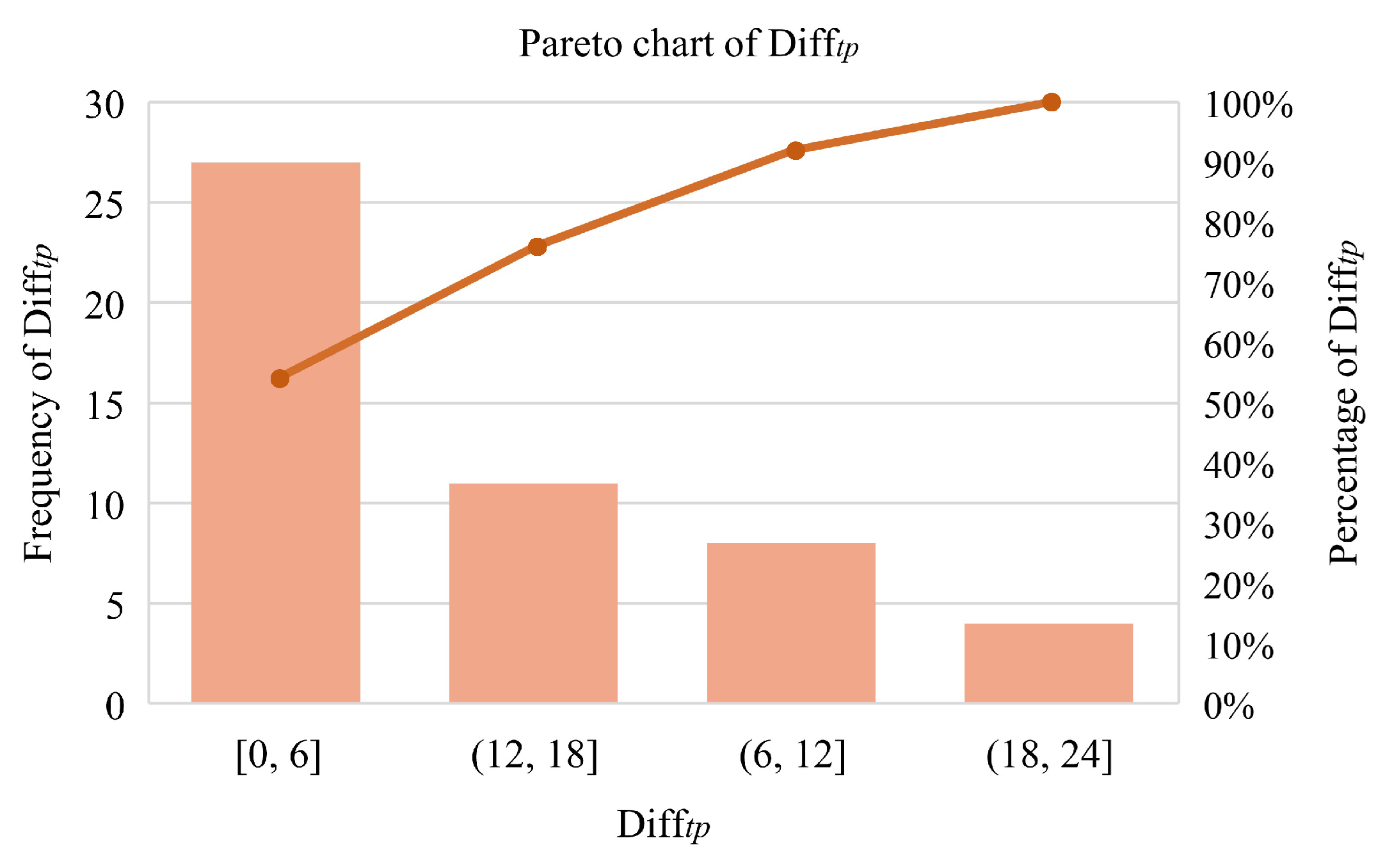
The value of n u m t p is 10 for data sets 1–5; therefore, there are 50 test patches in this subsection. The Pareto chart of Diff t p is shown in Figure 11. To objectively evaluate the effectiveness of the fitted curve N a = P 3 C , this paper puts forward the estimation accuracy (EA) curve evaluation criteria. By counting the frequency of these Diff t p and sorting them from small to large, we obtain:
Diff t p _ u = diff t p _ u 1 , , diff t p _ u h .
The abscissa of the EA curve is the Diff t p _ u , and the ordinate is the EA, which is defined as follows:
EA = N O P N O P A l l ,
where N O P represents the number of test patches of Diff t p Diff t p _ u , and N O P A l l represents the number of all test patches for evaluation.
Figure 12 shows the EA curves of P 1 C , P 2 C , and P 3 C based on data sets 1–5 and a randomly selected patch size. Moreover, data set 5 is not used for polynomial curve fitting. The EA curve shows that the differences Diff t p 2 of 24% test patches and 2 test patches are completely consistent with the optimal value N o for the P 3 C . When Diff t p _ u 5 , the EA curve rises sharply, and the difference Diff t p 6 of 54% test patches. The red line is clearly higher than the blue and green lines, which effectively shows the accuracy of P 3 C .When Diff t p _ u 15 , the accuracy set already contains 90% of the test patches, and only 8% of the test patches have a 20 Diff t p 23 . Data set 5 contains many kinds of terrain, such as water, buildings, and vegetation. Figure 8i shows that data set 5 is also seriously disturbed by noise. Figure 12b shows the EA curve of data set 5, which is superior to that of data sets 1–4. Moreover, the max Diff t p _ u of P 3 C is smaller than that of the P 1 C and P 2 C . The experiment results based on data set 5 verify the generalization ability of the proposed CEN.
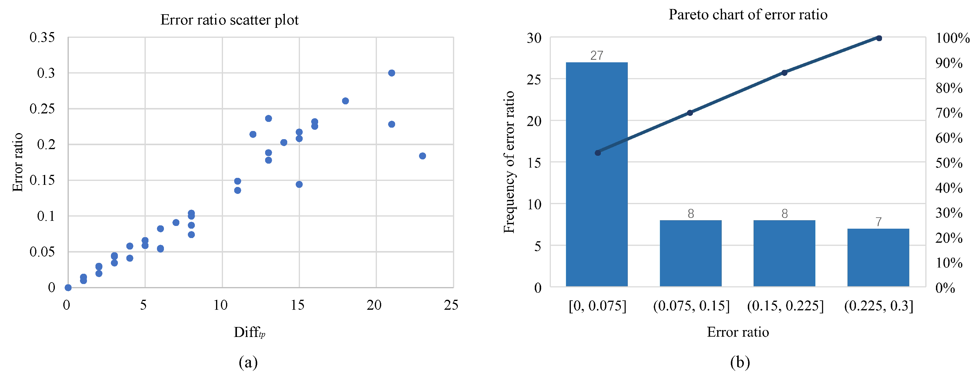
Figure 13a shows the error ratio scatter plot of P 3 C ; the abscissa is Diff t p _ u , and the ordinate is Diff t p _ u / N o , which is called the error ratio (ER), with a total of 5 × n u m t p scatter points. Figure 13b shows the ER 0.075 of 54% test patches, and a smaller ER shows that the accuracy of superpixel generation using N a and N o is almost similar; only three data points have an ER greater than 0.25.
Our proposed CEN achieves an EA of 92% when Diff t p 18 , and the ER is less than 0.26. The EA curve and the ER verify the universality and stability of the CEN algorithm to estimate adaptive N a via the structural complexity C . The proposed method does not need traversal parameters and greatly improves the computational efficiency of the parameter settings by utilizing superpixel generation for preprocessing. Meanwhile, the results verify that the proposed CEN has strong generalization ability and reliable estimation results for diverse data sets.

4.4. Superpixel Generation Results on Data Set 1

To verify the effictiveness of the proposed HADS, six comparison algorithms chosen from clustering-based methods were evaluated on data set 1, including POL-SLIC [26], POL-LSC [19], POL-HLT [10], HAGS [7], HAWS [30], and HAHS [10]. HAGS, HAHS, and HAWS adopt the same superpixel generation framework but different distance measurements. The parameter settings are as follows: 0.3 for POL-LSC, 0.1 for POL-SLIC, 1.8 for POL-HLT and HAHS, 0.13 for HAGS, 0.4 for HAWS, and m D R T = 1.4 for the proposed HADS.
According to Equation (12), the C of data set 1 is 0.521, and the adaptive N a is estimated using Equation (16) as shown in Table 3. Data set 1 contains more than 10 categories of terrain with high density and complex distribution [34]. Therefore, the ER of 0.05 ( n = 3 ) clearly demonstrates the reliability of the proposed CEN method to estimate N a of complex real-world PolSAR images. Therefore, HAGS, HAWS, HAHS, and HADS adopt the same superpixel generation framework with parameter N a = 68 . The initialization methods of POL-SLIC, POL-LSC and POL-HLT are the square distribution shown in Figure 7, so the value closest to N a , that is, S = 8 , is chosen. Figure 14 shows our proposed HADS method can obtain the smoothest superpixel boundary compared to the other six methods, where the average coherency matrix of the superpixel is the value of each pixel in the current superpixel.
Table 4 shows the evaluation results of data set 1, while Figure 15 and Figure 16 show the enlarged regions A and B in Figure 14. The BRs of POL-SLIC and POL-LSC are the worst, and the generated superpixels are irregular. Therefore, although POL-LSC has a lower time cost by MATLAB mixed with C code, the unsatisfactory segmentation results will lose the significance of superpixel generation and impact the efficiency of the interpretation. Both POL-HLT and HAHS utilize the HLT distance to generate superpixels; therefore, the BR, USE, and ASA are almost nondifferential. However, to satisfy the symmetric of the distance, calculating the HLT distance is time-consuming. Clearly, the RT of HAHS is 31% lower than that of POL-HLT because of the efficient initialization strategy. Moreover, Figure 15f and Figure 16f show the superiority of the hexagonal distribution with smoother edges. HAGS, HAWS, and the proposed HADS demonstrate the better performance of BR. Although the RT of HAGS has a slight advantage compared with that of HAWS and HADS, the BR and USE are clearly inferior. Figure 15d and Figure 16d also show that the HAGS is severely sensitive to speckle noise, such as the roads. Figure 15 demonstrates the ability of boundary adherence of HAWS and HADS to outperform others. However, our proposed HADS can preserve the detailed information better than HAWS in the blue rectangles of Figure 16. Moreover, the computational efficiency of HADS is 3% superior than that of HAWS, and the BR outperforms other competitive methods.
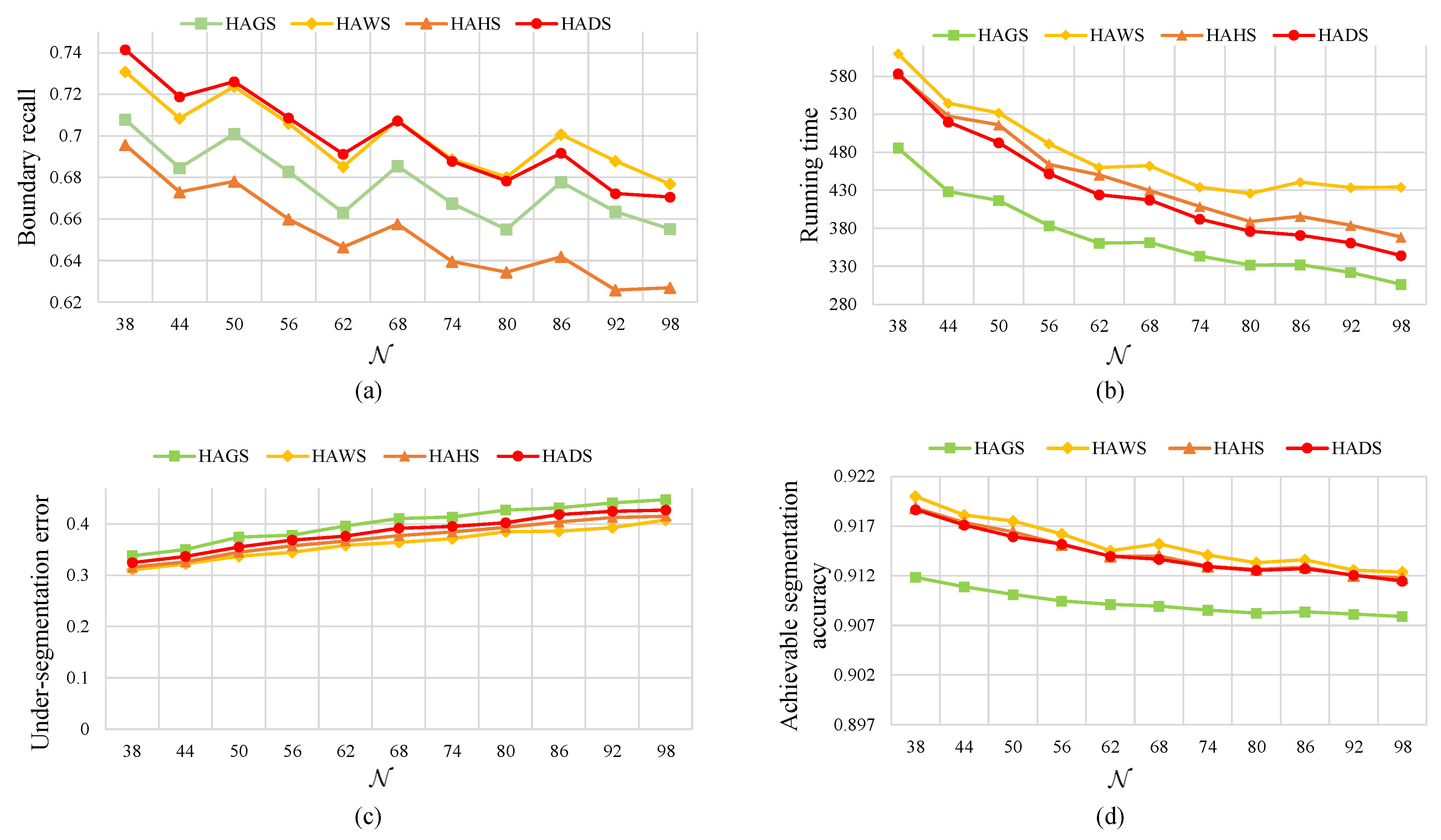
HAGS, HAWS, HAHS, and our proposed HADS adopt a similar superpixel generation framework with the same input parameter N a , for which only the distance measurement is different. To intuitively verify the effectiveness of the DRT distance, this subsection discusses a number of experiments based on the four competitive methods shown in Figure 17. The orange line representing HAHS is below the other lines in Figure 17a, which indicates inferior boundary adherence. The yellow and red lines are always intertwined and above the other lines, which demonstrates that HAWS and HADS can obtain superpixels with better performance of boundary adherence. Notably, the computational efficiency of HADS is superior to that of HAWS, as shown in Figure 17b. Moreover, not only is the adherent ability of HADS higher than that of HAHS, but the computational burden is also clearly lower. Figure 17b shows that the RT of HAGS outperforms the other methods because GD calculates the shortest distance between two pixels. However, the green line representing the proposed HADS is always approximately 6% higher than the HAGS, and Figure 15a and Figure 17 also show the irregular generated superpixels of HAGS. The USE and ASA of the four methods have no evident differences.
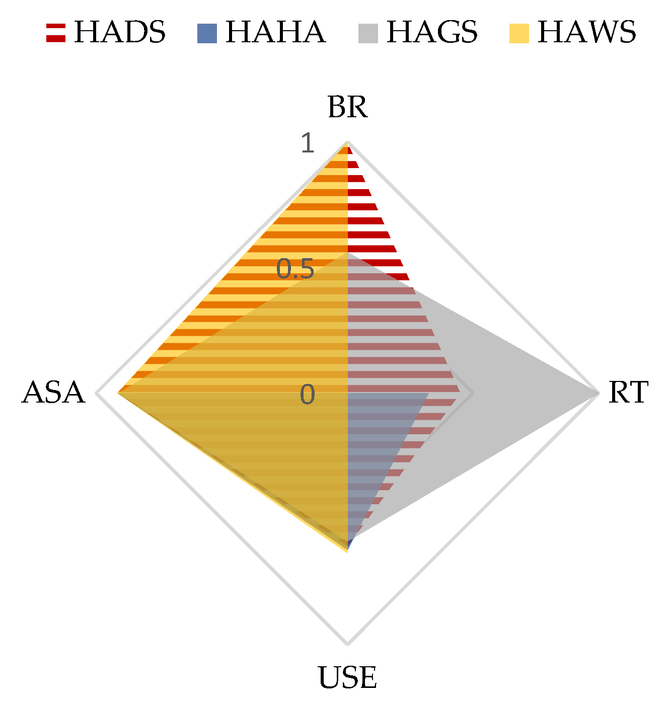
The results of data set 1 were inverted and normalized to construct a radar chart that can reflect the comprehensive performance of algorithms, as shown in Figure 18. The larger the value of each dimension of the radar chart, the better the segmentation performance. Superpixel generation is a preprocessing step of PolSAR image interpretation; therefore, the indispensable abilities are higher accuracy and lower computational burden. Figure 18 shows that the BR of HAHS is relatively poor, and the RT of HAWS is also lower than that of the other comparison methods. Moreover, the results of HAGS contain some blurred edges in Figure 15. Clearly, our proposed HADS can better balance segmentation accuracy and computational efficiency. When taking the value of N a = 65 , each algorithm not only owns a high value of BR, but also has a lower computational burden. The obtained superpixels can retain the details well, which fully verifies the effectiveness and feasibility of the proposed CEN in this paper.

4.5. Superpixel Generation Results on Data Set 5

This subsection details experiments conducted based on the actual PolSAR image of data set 5 with the six comparison methods mentioned above. Due to the noise interference in data set 5, the Lee filter was adopted to enhance the definition of the image with size w = 5 [39]. The parameter settings are as follows: 0.7 for POL-LSC, 0.1 for POL-SLIC, 4 for POL-HLT and HAHS, 0.3 for HAGS, 1.2 for HAWS, and m D R T = 1.4 for the proposed HADS.
According to Equation (12), C of data set 5 is 0.3213, and adaptive N a is estimated by Equation (16), as shown in Table 5. For visual analysis, the noise interference of data set 5 is serious compared with data sets 1–4. Therefore, the ER of 0.05 ( n = 3 ) illustrates the stability of the proposed CEN to estimate adaptive N a via the C under partially undesirable situations. Therefore, N a = 91 for HAGS, HAWS, HAHS, and HADS. The POL-SLIC, POL-LSC, and POL-HLT initialization methods are the square distribution shown in Figure 7, so the value closest to N a , that is, S = 10 , is chosen.
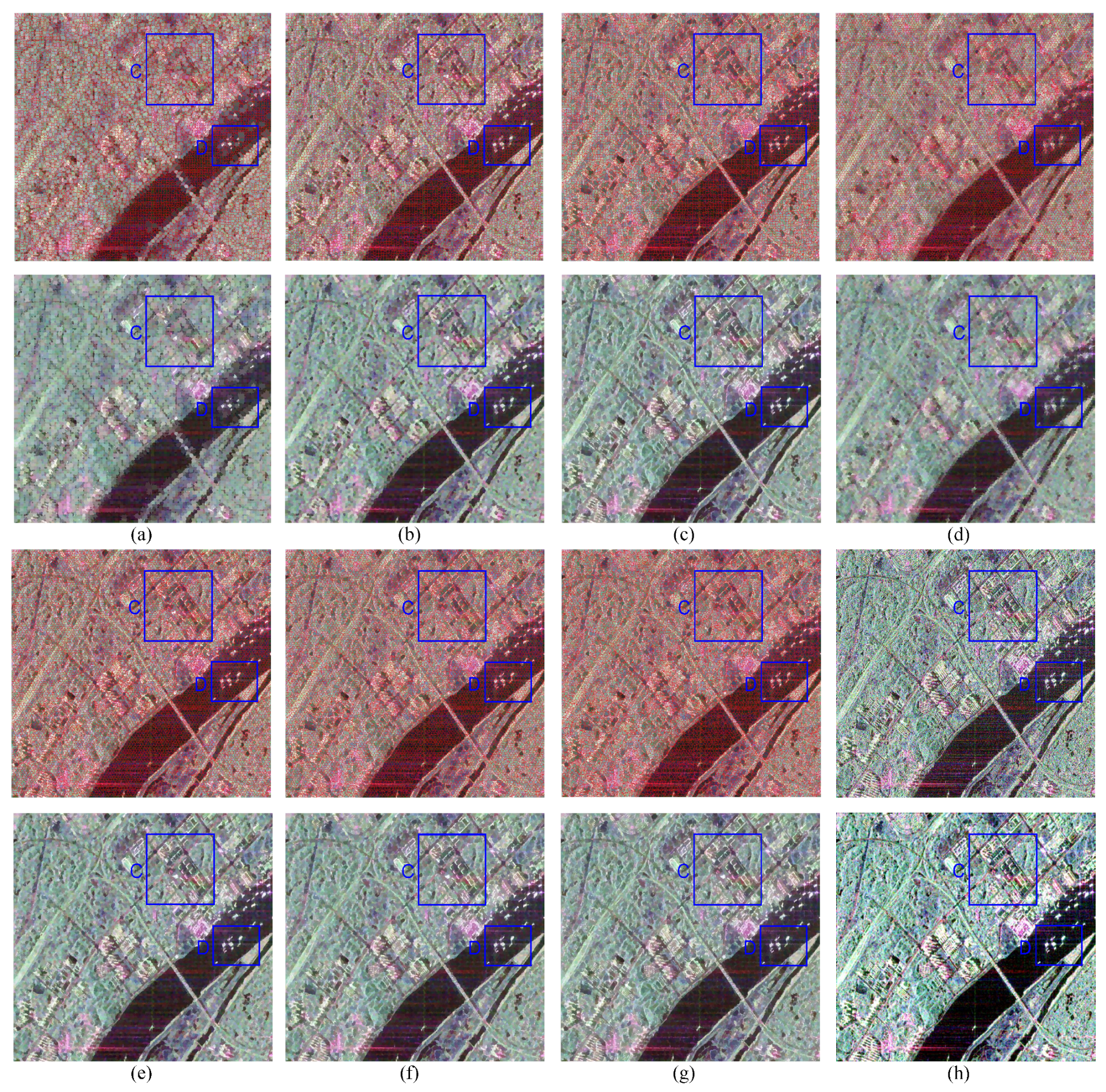
Figure 19 shows the results of the superpixel generation. The second row of Figure 19a–g shows the representation maps of different algorithms, where the average coherency matrix of the superpixel is the value of each pixel in the current superpixel. The first row of Figure 19a–g shows the corresponding superpixels with the red edges. Moreover, Figure 19h shows the unfiltered image and the filtered image with the size of w = 5 , respectively. POL-SLIC adopts the Wishart distance with a heavy computational burden to measure the similarity between pixels, and the square distribution also increases the number of distance calculations. Therefore, Table 6 shows the lower BR and higher RT of POL-SLIC.
Clearly, the filtering may slightly change the edge of the image. The calculation of the GD is greatly affected by filtering, and the boundary adherence of HAGS is slightly inferior to that of POL-LSC. However, Figure 19 illustrates that the generated superpixels of HAGS are more regular and closely arranged. Although the RT of POL-LSC is the smallest because of the mixed codes, the BR of POL-LSC has a large gap compared with our proposed HADS. The BR of HADS is 0.06 higher than that of POL-LSC. HAHS and POL-HLT adopt the HLT distance to generate superpixels, and the largest difference is the initialization. Therefore, Table 6 clearly shows the lighter computational burden of HAHS compared with POL-HLT. The BR of HAWS and our proposed HADS are superior to those of the other five competitive methods. Nevertheless, the computational efficiency of HADS obviously outperforms HAWS, and the RT of HADS is 33% smaller than that of HAWS. Figure 20 and Figure 21 show the enlarged two blue rectangles in Figure 19. Figure 21a,b shows the generated regular superpixels of POL-SLIC and POL-LSC; however, the boundary adherence ability is inferior, as shown in Figure 20. The blurred edges will create a loss of detail and reduce the efficiency of the subsequent interpretation steps. Figure 20 and Figure 21 show that the results of HAGS are severely affected by speckle noise. Compared with POL-HLT, HAWS, and HAHS, our proposed HADS can obtain more acceptable regularity and detailed edges shown as the blue rectangles in Figure 20.
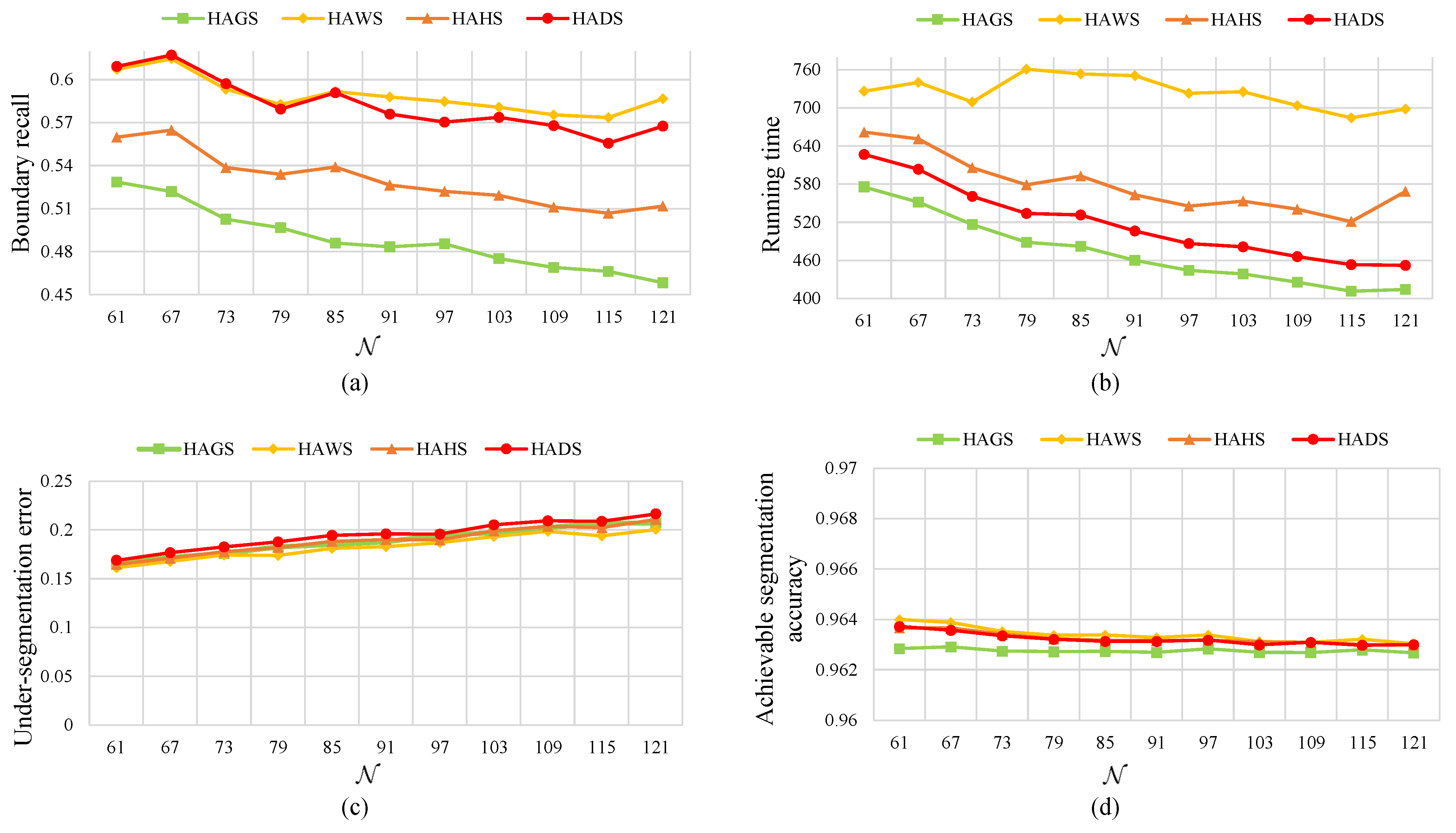
To verify the ability of the DRT distance, extensive experiments were conducted based on HAGS, HAWS, HAHS, and our proposed HADS on filtered data set 5. The USE and ASA in Figure 22 have no evident difference. The BR of HAGS is the lowest, but the computational burden is the smallest. Figure 22 shows the ordinary boundary adherence of HAHS, and the RT of HAHS is also unsatisfactory owing to the calculation of the HLT distance. The orange and red lines are always above the other lines, which represents the superiority of edge closeness for HAWS and HADS. However, the RT of HAWS is the poorest. Figure 23 shows the radar chart of data set 5. The BR of HAGS and the RT of HAWS are the worst among the four methods. Moreover, the BR and RT of the HAHS are inferior to that of the proposed HADS. It cannot be denied that the proposed HADS is capable of balancing accuracy and computational efficiency. The RT of HADS is 33% lower than that of HAWS when N = N a . Figure 22 verifies that the proposed HADS is capable of balancing the time consumed and segmentation accuracy. Furthermore, Figure 22 shows that when N = N a , each algorithm is capable of adhering closely to the edges and retaining superior computational efficiency, which demonstrates the accuracy of the proposed CEN.

5. Conclusions

Most superpixel generation methods for PolSAR images should set the initial superpixel size. The initial superpixel size commonly has a great impact on the boundary adherence, and some unreasonable selections with small empirical values may increase the calculation time. Therefore, this paper proposes to define the function expression between the structural complexity of PolSAR images and the adaptive number of pixels contained in the initial superpixel. Moreover, comprehensive evaluation criteria are proposed to select N a for constructing numerous sample points that are utilized to fit the generalized polynomial. Clustering-based superpixel generation methods are attractive because of their feasibility and controllability. Actually, the distance measurement plays a key role in clustering-based methods. The modeling capabilities and the simple calculation of the DRT distance are crucial for generating superpixels of PolSAR images.
Quantitative performance evaluations on three AIRSAR data sets, one ESAR data set, and one Gaofen-3 PolSAR data set demonstrate the generalization of the proposed CEN and the availability of the proposed HADS in terms of four commonly used criteria, i.e., the BR, RT, USE, and ASA. In total, 559 sample points from five real-world data sets were used to fit the reliable polynomial curve, and the new evaluation of the EA curve and the ER demonstrate the universality of the CEN. Among the six state-of-the-art PolSAR image superpixel generation algorithms, using either unfiltered or filtered data, the proposed HADS outperforms other algorithms with a better balance between computational efficiency and segmentation accuracy. In our future work, other excellent distance measurements can be adopted to enhance the segmentation performance for PolSAR images.

Author Contributions

Conceptualization, M.L. and H.Z.; methodology, M.L.; software, M.L.; validation, M.L. and X.Q.; formal analysis, M.L. and Z.D.; investigation, M.L.; resources, H.Z. and Z.D.; data curation, M.L. and H.Z.; writing—original draft preparation, M.L.; writing—review and editing, M.L. and X.Q.; visualization, L.S. and J.W.; supervision, H.Z. and Z.D. All authors have read and agreed to the published version of the manuscript.

Funding

This work was supported by the National Natural Science Foundation of China under Grant 62071474 and in part by the Natural Science Basic Research Plan in Shaanxi Province 2022JM-157 and the China Postdoctoral Science Foundation 2021M702672.

Data Availability Statement

Not applicable.

Conflicts of Interest

The authors declare no conflict of interest.

References

  1. Ren, S.; Zhou, F. Semi-Supervised Classification for PolSAR Data With Multi-Scale Evolving Weighted Graph Convolutional Network. IEEE J. Sel. Top. Appl. Earth Obs. Remote Sens. 2021, 14, 2911–2927. [Google Scholar] [CrossRef]
  2. Zhang, T.; Du, Y.; Yang, Z.; Quan, S.; Liu, T.; Xue, F.; Chen, Z.; Yang, J. PolSAR Ship Detection Using the Superpixel-Based Neighborhood Polarimetric Covariance Matrices. IEEE Geosci. Remote Sens. Lett. 2021, 19, 1–5. [Google Scholar] [CrossRef]
  3. Gadhiya, T.; Roy, A.K. Superpixel-Driven Optimized Wishart Network for Fast PolSAR Image Classification Using Global k-Means Algorithm. IEEE Trans. Geosci. Remote Sens. 2019, 58, 97–109. [Google Scholar] [CrossRef]
  4. Bi, H.; Sun, J.; Xu, Z. A Graph-Based Semisupervised Deep Learning Model for PolSAR Image Classification. IEEE Trans. Geosci. Remote Sens. 2019, 57, 2116–2132. [Google Scholar] [CrossRef]
  5. Tan, W.; Sun, B.; Xiao, C.; Huang, P.; Yang, W. A Novel Unsupervised Classification Method for Sandy Land Using Fully Polarimetric SAR Data. Remote Sens. 2021, 13, 355. [Google Scholar] [CrossRef]
  6. Meilin, L.; Huanxin, Z.; Qian, M.; Jiachi, S.; Xu, C.; Xianxiang, Q. Unsupervised classification of PolSAR image based on tensor product graph diffusion. Proc. SPIE 2019, 11198, 1–6. [Google Scholar]
  7. Stutz, D.; Hermans, A.; Leibe, B. Superpixels: An evaluation of the state-of-the-art. Comput. Vis. Image Underst. CVIU 2018, 166, 1–27. [Google Scholar] [CrossRef] [Green Version]
  8. Achanta, R.; Shaji, A.; Smith, K.; Lucchi, A.; Fua, P.; Sstrunk, S. SLIC Superpixels Compared to State-of-the-Art Superpixel Methods. IEEE Trans. Pattern Anal. Mach. Intell. 2012, 34, 2274–2282. [Google Scholar] [CrossRef] [Green Version]
  9. Quan, S.; Xiang, D.; Wang, W.; Xiong, B.; Kuang, G. Scattering Feature-Driven Superpixel Segmentation for Polarimetric SAR Images. IEEE J. Sel. Top. Appl. Earth Obs. Remote Sens. 2021, 14, 2173–2183. [Google Scholar] [CrossRef]
  10. Yin, J.; Wang, T.; Du, Y.; Liu, X.; Zhou, L.; Yang, J. SLIC Superpixel Segmentation for Polarimetric SAR Images. IEEE Trans. Geosci. Remote. Sens. 2021, 60, 1–17. [Google Scholar] [CrossRef]
  11. Xiang, D.; Wang, W.; Tang, T.; Guan, D.; Quan, S.; Liu, T.; Su, Y. Adaptive Statistical Superpixel Merging With Edge Penalty for PolSAR Image Segmentation. IEEE Trans. Geosci. Remote Sens. 2020, 58, 2412–2429. [Google Scholar] [CrossRef]
  12. Gao, H.; Wang, C.; Xiang, D.; Ye, J.; Wang, G. TSPol-ASLIC: Adaptive Superpixel Generation With Local Iterative Clustering for Time-Series Quad- and Dual-Polarization SAR Data. IEEE Trans. Geosci. Remote Sens. 2022, 60, 1–15. [Google Scholar] [CrossRef]
  13. Comaniciu, D.; Meer, P. Mean shift analysis and applications. In Proceedings of the IEEE International Conference on Computer Vision, Washington, DC, USA, 3–6 December 2002. [Google Scholar]
  14. Tuzel, M.; Ramalingam, O.; Liu, M.; Tuzel, O.; Ramalingam, S. Entropy rate superpixel segmentation. In Proceedings of the CVPR 2011, Colorado Springs, CO, USA, 20–25 June 2011. [Google Scholar]
  15. Zhang, Y.; Hartley, R.; Mashford, J.; Burn, S. Superpixels via pseudo-Boolean optimization. In Proceedings of the 2011 IEEE International Conference on Computer Vision (ICCV), Barcelona, Spain, 6–13 November 2011; pp. 1387–1394. [Google Scholar]
  16. Levinshtein, A.; Stere, A.; Kutulakos, K.N.; Fleet, D.J.; Siddiqi, K. TurboPixels: Fast Superpixels Using Geometric Flows. IEEE Trans. Pattern Anal. Mach. Intell. 2009, 31, 2290–2297. [Google Scholar] [CrossRef] [Green Version]
  17. Nock, R.; Nielsen, F. Statistical region merging. IEEE Trans. Pattern Anal. Mach. Intell. 2004, 26, 1452. [Google Scholar] [CrossRef]
  18. Yang, S.; Yuan, X.; Liu, X.; Chen, Q. Superpixel generation for polarimetric SAR using Hierarchical Energy maximization. Comput. Geosci. 2019, 135. [Google Scholar] [CrossRef]
  19. Li, Z.; Chen, J. Superpixel segmentation using Linear Spectral Clustering. In Proceedings of the 2015 IEEE Conference on Computer Vision and Pattern Recognition (CVPR), Boston, MA, USA, 7–12 June 2015. [Google Scholar]
  20. Liu, B.; Hu, H.; Wang, H.; Wang, K.; Liu, X.; Yu, W. Superpixel-Based Classification With an Adaptive Number of Classes for Polarimetric SAR Images. IEEE Trans. Geosci. Remote Sens. 2013, 51, 907–924. [Google Scholar] [CrossRef]
  21. Wang, W.; Xiang, D.; Ban, Y.; Zhang, J.; Wan, J. Superpixel Segmentation of Polarimetric SAR Data Based on Integrated Distance Measure and Entropy Rate Method. IEEE J. Sel. Top. Appl. Earth Obs. Remote Sens. 2017, 10, 4045–4058. [Google Scholar] [CrossRef]
  22. Lang, F.; Yang, J.; Li, D.; Shi, L.; Wei, J. Mean-Shift-Based Speckle Filtering of Polarimetric SAR Data. IEEE Trans. Geosci. Remote. Sens. 2014, 52, 4440–4454. [Google Scholar] [CrossRef]
  23. Fengkai, L.; Jie, Y.; Shiyong, Y.; Fachao, Q. Superpixel Segmentation of Polarimetric Synthetic Aperture Radar (SAR) Images Based on Generalized Mean Shift. Remote Sens. 2018, 10, 1592. [Google Scholar]
  24. Hu, H.; Liu, B.; Zhang, Z.; Guo, W.; Yu, W. Superpixel generation for synthetic aperture radar imagery using edge-dominated local clustering. J. Appl. Remote Sens. 2018, 12, 045006. [Google Scholar] [CrossRef]
  25. Bagrov, A.A.; Iakovlev, I.A.; Iliasov, A.A.; Katsnelson, M.I.; Mazurenko, V.V. Multiscale structural complexity of natural patterns. Proc. Natl. Acad. Sci. USA 2020, 117, 30241–30251. [Google Scholar] [CrossRef]
  26. Feng, J.; Cao, Z.; Pi, Y. Polarimetric Contextual Classification of PolSAR Images Using Sparse Representation and Superpixels. Remote Sens. 2014, 6, 7158–7181. [Google Scholar] [CrossRef] [Green Version]
  27. Qin, F.; Guo, J.; Lang, F. Superpixel Segmentation for Polarimetric SAR Imagery Using Local Iterative Clustering. IEEE Geosci. Remote Sens. Lett. 2017, 12, 13–17. [Google Scholar]
  28. Yue, Z.; Zou, H.; Luo, T.; Qin, X.; Zhou, S.; Ji, K. A Fast Superpixel Segmentation Algorithm for PolSAR Images Based on Edge Refinement and Revised Wishart Distance. Sensors 2016, 16, 1687. [Google Scholar]
  29. Zhu, S.; Cao, D.; Jiang, S.; Wu, Y.; Hu, P. Fast superpixel segmentation by iterative edge refinement. Electron. Lett. 2015, 51, 230–232. [Google Scholar] [CrossRef]
  30. Li, M.; Zou, H.; Ma, Q.; Sun, J.; Qin, X. Superpixel Segmentation for PolSAR Images Based on Hexagon Initialization and Edge Refinement. In Proceedings of the ISPRS Archives, Virtual Event, 7–8 October 2020. [Google Scholar]
  31. Ratha, D.; De, S.; Celik, T.; Bhattacharya, A. Change Detection in Polarimetric SAR Images Using a Geodesic Distance Between Scattering Mechanisms. IEEE Geosci. Remote Sens. Lett. 2017, 14, 1040–1066. [Google Scholar] [CrossRef]
  32. Akbari, V.; Anfinsen, S.N.; Doulgeris, A.P.; Eltoft, T.; Moser, G.; Serpico, S.B. Polarimetric SAR Change Detection With the Complex Hotelling–Lawley Trace Statistic. IEEE Trans. Geosci. Remote Sens. 2016, 54, 3953–3966. [Google Scholar] [CrossRef] [Green Version]
  33. Bouhlel, N.; Akbari, V.; Méric, S. Change Detection in Multilook Polarimetric SAR Imagery With Determinant Ratio Test Statistic. IEEE Trans. Geosci. Remote Sens. 2022, 60, 1–15. [Google Scholar] [CrossRef]
  34. Qin, X.; Zou, H.; Yu, W.; Wang, P. Superpixel-Oriented Classification of PolSAR Images Using Complex-Valued Convolutional Neural Network Driven by Hybrid Data. IEEE Trans. Geosci. Remote Sens. 2020, 59, 10094–10111. [Google Scholar] [CrossRef]
  35. Goodman, N.R. Statistical Analysis Based on a Certain Multivariate Complex Gaussian Distribution. Ann. Math. Stat. 1963, 34, 152–177. [Google Scholar] [CrossRef]
  36. Li, M.; Zou, H.; Qin, X.; Dong, Z.; Sun, L.; Wei, J. Efficient Superpixel Generation for Polarimetric SAR Images with Cross-Iteration and Hexagonal Initialization. Remote Sens. 2022, 14, 2914. [Google Scholar] [CrossRef]
  37. Yang, Y.; Xu, T.; Sun, Z.; Nie, W.; Fang, Z. Middle- and Long-Term UT1-UTC Prediction Based on Constrained Polynomial Curve Fitting, Weighted Least Squares and Autoregressive Combination Model. Remote Sens. 2022, 14, 3252. [Google Scholar] [CrossRef]
  38. Ai, J.; Wang, F.; Mao, Y.; Luo, Q.; Yao, B.; Yan, H.; Xing, M.; Wu, Y. A Fine PolSAR Terrain Classification Algorithm Using the Texture Feature Fusion-Based Improved Convolutional Autoencoder. IEEE Trans. Geosci. Remote Sens. 2022, 60, 1–14. [Google Scholar] [CrossRef]
  39. Yommy, A.S.; Liu, R.; Wu, A.S. SAR Image Despeckling Using Refined Lee Filter. In Proceedings of the International Conference on Intelligent Human-Machine Systems and Cybernetics, Hangzhou, China, 26–27 August 2015. [Google Scholar]
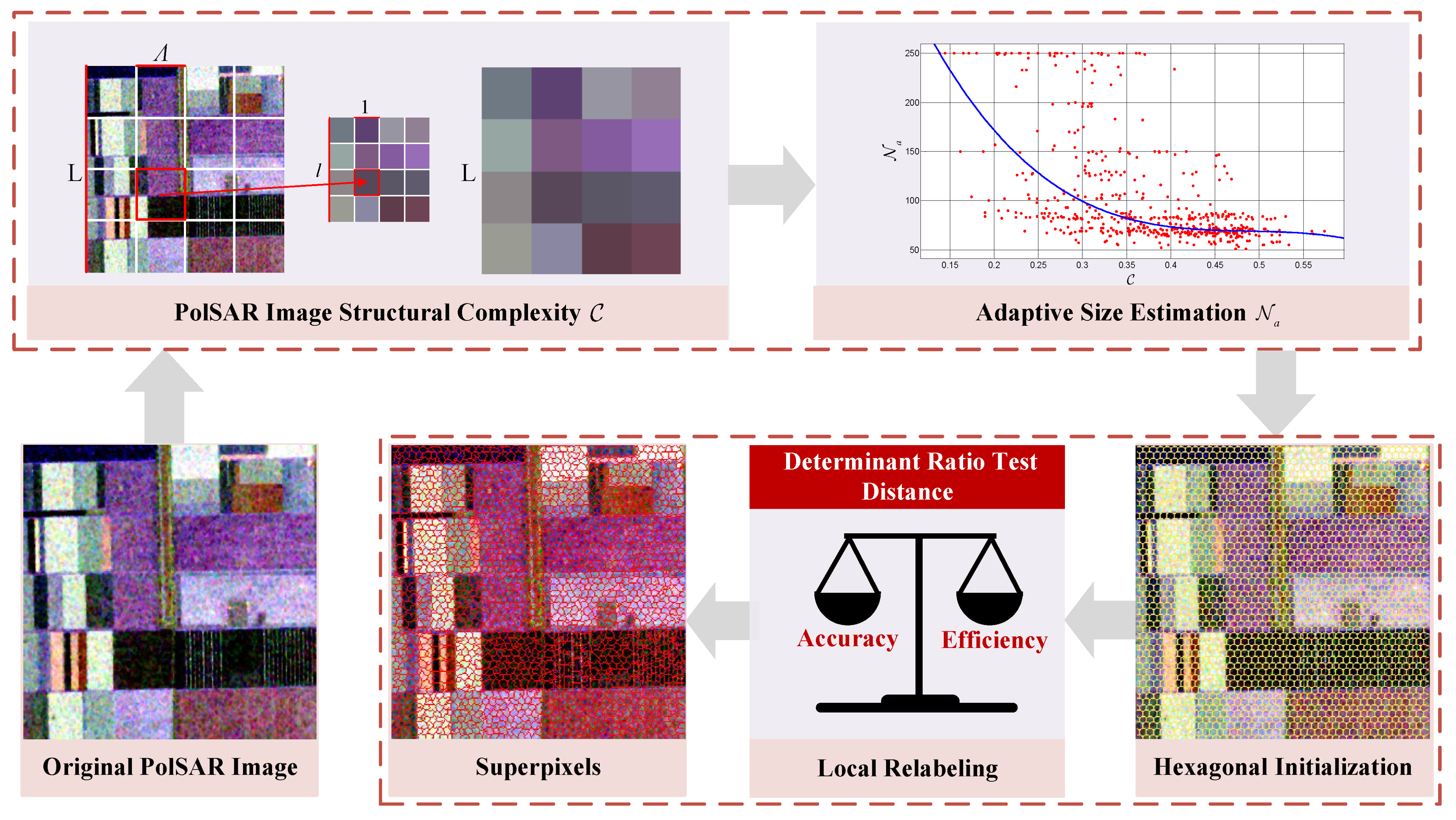
Figure 1. An overview of the proposed method.
Remotesensing 15 01123 g001
Figure 2. An example of an AIRSAR L-Band PolSAR image. (a) The AIRSAR L-Band PolSAR image. (b) Enlarged region A. (c) Enlarged region B.
Remotesensing 15 01123 g002
Figure 3. Schematic representation of the PolSAR image’s structural complexity. A PolSAR image of L × L pixels (I) is divided into blocks of Λ × Λ pixels (II). A renormalized image of l × l pixels is plotted, where l = L / Λ ( l = 4 , Λ = 2 in this paper). The renormalized image is rescaled up to the initial image size (III). Vectors A and B are constructed from blocks of the initial and the renormalized images, respectively (IV). The scalar product of these vectors is used to define overlap O. For illustrative purposes, pixelwise products of A and B blocks are shown as vector O.
Remotesensing 15 01123 g003
Figure 4. Results of IER based on hexagonal initialization of the 300 × 300 pixel simulated PolSAR image. (a) Pauli-RGB image. (b) Generated superpixels of N = 36 ; the RT is 32 s. (c) Generated superpixels of N = 64 ; the RT is 29 s.
Remotesensing 15 01123 g004
Figure 5. Results of IER based on hexagonal initialization of the 512 × 512 pixel simulated PolSAR image. (a) Pauli-RGB image. (b) Generated superpixels of N = 64 ; the RT is 85 s. (c) Generated superpixels of N = 100 ; the RT is 74 s.
Remotesensing 15 01123 g005
Figure 6. Flowchart of the proposed CEN and the proposed HADS.
Remotesensing 15 01123 g006
Figure 7. Distribution of cluster centers. (a) Square distribution. (b) Hexagonal distribution.
Remotesensing 15 01123 g007
Figure 8. Data sets 1–5. (a,c,e,g,i) are the Pauli-RGB images of data sets 1–5. (b,d,f,h,j) are ground-truth maps of data sets 1–5.
Remotesensing 15 01123 g008
Figure 9. Some examples of patches used for polynomial curve fitting from data sets 1–4. (ad) are the patches of 512 × 512 pixels, and (eh) are the patches of 256 × 256 pixels. The values of complexity C are 0.4536, 0.4582, 0.3196, 0.5612, 0.4503, 0.3814, 0.1616, and 0.3545, respectively.
Remotesensing 15 01123 g009
Figure 10. Polynomial curve N a = P n C between the complexity C and the estimated N a .
Remotesensing 15 01123 g010
Figure 11. Pareto chart of Diff t p of the fitted curve N a = P 3 C .
Remotesensing 15 01123 g011
Figure 12. Estimation accuracy of the three fitted curves. (a) Estimation accuracy based on data sets 1–5. (b) Estimation accuracy based on data set 5.
Remotesensing 15 01123 g012
Figure 13. Results of error ratio. (a) Error ratio scatter plot. (b) Pareto chart of error ratio.
Remotesensing 15 01123 g013
Figure 14. Qualitative evaluation results of data set 1. (a) POL-SLIC. (b) POL-LSC. (c) POL-HLT. (d) HAGS. (e) HAWS. (f) HAHS. (g) The proposed HADS. (h) Pauli-RGB image.
Remotesensing 15 01123 g014
Figure 15. Enlarged results for region A of data set 1. (a) POL-SLIC. (b) POL-LSC. (c) POL-HLT. (d) HAGS. (e) HAWS. (f) HAHS. (g) The proposed HADS. (h) Pauli-RGB image.
Remotesensing 15 01123 g015
Figure 16. Enlarged results for region B of data set 1. (a) POL-SLIC. (b) POL-LSC. (c) POL-HLT. (d) HAGS. (e) HAWS. (f) HAHS. (g) The proposed HADS. (h) Pauli-RGB image.
Remotesensing 15 01123 g016
Figure 17. Quantitative evaluation results based on data set 1. (a) BR. (b) RT(s). (c) USE. (d) ASA.
Remotesensing 15 01123 g017
Figure 18. The radar chart of data set 1 when N a = 65 .
Remotesensing 15 01123 g018
Figure 19. Qualitative evaluation results of data set 5. (a) POL-SLIC. (b) POL-LSC. (c) POL-HLT. (d) HAGS. (e) HAWS. (f) HAHS. (g) The proposed HADS. (h) Pauli-RGB image.
Remotesensing 15 01123 g019
Figure 20. Enlarged results for region C of data set 5. (a) POL-SLIC. (b) POL-LSC. (c) POL-HLT. (d) HAGS. (e) HAWS. (f) HAHS. (g) The proposed HADS. (h) Pauli-RGB image.
Remotesensing 15 01123 g020
Figure 21. Enlarged results for region D of data set 5. (a) POL-SLIC. (b) POL-LSC. (c) POL-HLT. (d) HAGS. (e) HAWS. (f) HAHS. (g) The proposed HADS. (h) Unfiltered Pauli-RGB image.
Remotesensing 15 01123 g021
Figure 22. Quantitative evaluation results based on data set 5. (a) BR. (b) RT(s). (c) USE. (d) ASA.
Remotesensing 15 01123 g022
Figure 23. The radar chart of data set 5 when N a = 91 .
Remotesensing 15 01123 g023
Table 1. Some information on experimental PolSAR data sets.
DescriptionData Set 1Data Set 2Data Set 3Data Set 4Data Set 5
OrganizationNASA/JPLNASA/JPLNASA/JPLDLRCASC
SystemAIRSARAIRSARAIRSARESARGaofen-3
LocationFlevolandFlevolandSan FranciscoOberpfaffenhofenChangsha
Imaging year19911989-19992017
BandLLCLC
Resolution∼ 12 × 6 m---8 m
Size750 × 1024768 × 1024900 × 10241300 × 12001000 × 1000
Table 2. Some details of image patches from data sets 1–4.
Data SetsPatch Size max C pc min C pc C expdiff Number of
Patches
num sup _ 1 , num sup _ w Number of
Superpixel
Generation
Data set 1512 × 512
256 × 256
0.066
0.207
0.00321
63
25 , 250 21 × 226
63 × 226
Data set 2512 × 512
256 × 256
0.080
0.208
0.00328
63
25 , 250 28 × 226
63 × 226
Data set 3512 × 512
256 × 256
0.187
0.305
0.00363
99
25 , 250 63 × 226
99 × 226
Data set 4512 × 512
256 × 256
0.286
0.384
0.00390
132
25 , 250 90 × 226
132 × 226
Table 3. Estimation results of data set 1.
N o C n N a EREA ( Diff tp _ u = 5 )EA ( Diff tp _ u = 15 )
650.52161
2
3
58
70
68
0.10
0.08
0 . 05
13%
49%
49 %
76%
78%
86 %
Note: The results of the proposed P3(C) are in bold faces.
Table 4. Four evaluation criteria for 7 methods based on data set 1.
MethodsPOL-SLICPOL-LSCPOL-HLTHAGSHAWSHAHSHADS
Criteria
BR0.510.610.670.690.710.660.71
RT(s)831.50203.44603.19361.41462.35429.69417.08
USE0.370.370.380.410.360.380.39
ASA0.910.910.910.910.920.910.91
Note: The results of the proposed HADS in bold faces.
Table 5. Estimation results for data set 5.
N o C n N a EREA ( Diff tp _ u = 5 )EA ( Diff tp _ u = 15 )
870.32131
2
3
93
94
91
0.07
0.09
0 . 05
13%
48%
50 %
77%
79%
87 %
Note: The results of the proposed P3(C) in bold faces.
Table 6. Four evaluation criteria for 7 methods based on the filtered data set 5 using Lee filter with w = 5 .
MethodsPOL-SLICPOL-LSCPOL-HLTHAGSHAWSHAHSHADS
Criteria
BR0.370.520.540.480.590.530.58
RT(s)1085.21255.90752.99460.02750.68562.82506.24
USE0.230.200.200.190.180.190.20
ASA0.960.960.960.960.960.960.96
Note: The results of the proposed HADS in bold faces.
Disclaimer/Publisher’s Note: The statements, opinions and data contained in all publications are solely those of the individual author(s) and contributor(s) and not of MDPI and/or the editor(s). MDPI and/or the editor(s) disclaim responsibility for any injury to people or property resulting from any ideas, methods, instructions or products referred to in the content.