Article

Assessment of Irrigation Demands Based on Soil Moisture Deficits Using a Satellite-Based Hydrological Model

Department of Agricultural and Food Engineering, Indian Institute of Technology Kharagpur, Kharagpur 721302, India
*
Author to whom correspondence should be addressed.
Remote Sens. 2023, 15(4), 1119; https://doi.org/10.3390/rs15041119
Submission received: 27 December 2022 / Revised: 2 February 2023 / Accepted: 16 February 2023 / Published: 18 February 2023

Abstract

:
Soil moisture deficit is an essential element in the estimation of irrigation demands, both spatially and temporarily. The determination of temporal and spatial variations of soil moisture in a river basin is challenging in many aspects; however, distributed hydrological modelling with remote sensing inputs is an effective way to determine soil moisture. In this research, a water demand module was developed for a satellite-based National Hydrological Model—India (NHM-I) to estimate distributed irrigation demands based on soil moisture deficits. The NHM-I is a conceptual distributed model that was explicitly developed to utilize the products from remote sensing satellites. MOD13Q1.5 data were used in this study to classify paddy and irrigated dry crops. Along with the above data, the DEM, Leaf Area Index, FAO soil map, and crop characteristics data were also used as inputs. The NHM-I with water demand module was evaluated in the Damodar river basin, India, from 2009 to 2018. The integrated NHM-I model simulated the irrigation demands effectively with remote sensing data. The temporal analysis reveals that soil moisture deficits in the Kharif season varied annually from 2009 to 2018; however, soil moisture deficits in the Rabi season were almost constant. The 50% Allowable Moisture Depletion (AMD-50) scenario can reduce the irrigation demand of 1966 MCM compared to the Zero Allowable Moisture Depletion (AMD-0) scenario. The highest annual irrigation demand (8923 MCM) under the AMD-50 scenario occurred in the 2015–2016 season, while the lowest (6344 MCM) happened in 2013–2014 season. With a new water demand module and remote sensing inputs, the NHM-I will provide a platform to assess spatial and temporal irrigation demands and soil moisture.

1. Introduction

Water is crucial for a region’s development, planning, and management in the 21st century. Demand for irrigation water is rising quickly due to climate change and the increasing global population [1]. Understanding the dynamics of human–water interactions in both time and space requires estimating the irrigation water demands in a river basin [2,3]. The assessment of current and future irrigation water demands using water balance approaches can be supported by estimates of soil moisture together with estimations of evapotranspiration [4]. Soil moisture deficit due to evapotranspiration is essential in estimating spatial and temporal irrigation demands. However, determining temporal and spatial variations of soil moisture in a river basin is challenging.
The fast growth of remote sensing technologies in previous decades has made it possible to collect spatial soil moisture from space. Numerous investigations, from the optical to the microwave areas, have shown the capacity and potential to determine soil moisture using different electromagnetic spectrums [5,6,7]. Based on the electromagnetic radiation’s sensing depths, the soil moisture obtained by these remote sensing techniques is referred to as surface or near-surface moisture [8]. These techniques may not capture the soil moisture variations in the root zone. Although soil moisture estimation in the root zone has been the subject of several studies, most of these methods use surface moisture as an input to establish connections with root zone soil moisture [9,10,11]. In this context, a hydrological model with suitable remote sensing inputs provides a reasonable estimation of variations in soil moisture and, thus, of irrigation demands over space and time [12].
Understanding the effects of anthropogenic activities on the water balance and water resources management can be achieved by hydrological modelling. Distributed hydrological models effectively simulate the water balance among all hydrological components, including spatial variations in surface water and groundwater [13,14,15]. Distributed hydrological modelling with water demand components is necessary and is a better technique for effective water management in a river basin [16]. The irrigation demands in these distributed hydrological models are represented using crop water requirements and effective rainfall [17,18,19,20,21,22]. However, no study has reported representing the irrigation demands based on the soil moisture deficit in a hydrological model.
Examining the temporal and spatial variations of irrigation demands is essential for effectively distributing water resources. This assessment also forms the basis for evaluating the potential for agricultural water savings [23]. Few model-independent studies used the concept of crop water requirements and effective rainfall to assess the temporal and spatial variations of irrigation demands [23,24,25,26]. However, these studies did not explicitly consider soil moisture deficits and other hydrological processes. Thus, limited research is available on assessing temporal and spatial variations of irrigation demand using a distributed hydrological model, especially under different soil moisture deficits.
Assessing and managing water resources using conventional methods in India is difficult. Therefore, a comprehensive hydrological modelling framework for the entire topography of India is desirable. National Hydrological Model—India (NHM-I), formerly known as the Satellite-based Hydrological Model, is a fully distributed conceptual hydrological model developed for the Indian landmass [14]. The NHM-I model primarily concentrates on the spatial distribution of hydrological variables for evaluating effective water resource management at the scale of river basins. A water demand module that can estimate the irrigation water demands is needed within the NHM-I for effective water management in a river basin and the command area.
Based on the identified research gaps above, the novelty of this study lies in estimating irrigation demands based on soil moisture deficits using a distributed hydrological model and assessing temporal and spatial variations of irrigation demand under different soil moisture deficits. The objectives of this study are 1. To develop a water demand module for the NHM-I model; 2. To assess irrigation demand’s temporal and spatial variations using the water demand module in a river basin.

2. Materials and Methods

2.1. Study Area

The Damodar River basin, a reservoir-regulated basin (Figure 1), is situated at the boundary of West Bengal and Jharkhand, India (22°45′N–24°30′N; 84°45′E–88°00′E). The Damodar River basin has a catchment area of 19,673 km2. The river basin receives 1250 mm of rainfall on average per year, with the monsoon season (June to September) accounting for 80% of that total. The study area experiences a tropical environment with an average temperature of 30 °C, rising to a maximum to 48 °C from May to July. The temperature in winter can drop as low as −2 °C. The Damodar river basin has five reservoirs: Tenughat, Konar, Tilaya, Panchet, and Maithon. The agricultural area is the dominant land cover in the study area, with an area of 13,152 km2, followed by forest (3846 km2). Paddy is the main crop in the study area during the Kharif season (June to October). Apart from the paddy, maize and seasonal vegetables are cultivated. However, potatoes, millets, and pulses are major crops in the Rabi season (November–February). Most people live in rural areas and depend heavily on agriculture in the study area. The Damodar river is the perennial water source in the basin, while the Barakar river, a tributary of the Damodar river, is an intermittent secondary source.

2.2. Data Used

From the USGS Earth Explorer website, a 30 m high-resolution Digital Elevation Model (DEM) was downloaded to assess the topographic characteristics (https://earthexplorer.usgs.gov/, accessed on 1 December 2022) (Figure 1). From 2009 to 2018, maximum and minimum temperature data (1° × 1°) and daily gridded rainfall data (0.25° × 0.25°) were downloaded from the website of the India Meteorological Department (IMD). For crop classification, this study used the MOD13Q1.5 product, which provides an every 16-day composite picture obtained by the MODIS sensor with a spatial resolution of 250 m. The satellite imageries of MODIS were classified by Gumma et al. [27] at International Crops Research Institute for the Semi-Arid Tropics (ICRISAT), Hyderabad. In the classification, ideal spectra of paddy were created, utilizing every 16-day MODIS NDVI time-series data and detailed knowledge on croplands based on extensive ground survey data. Class spectra were produced by unsupervised classification of MODIS NDVI time-series data using the ISOCLASS cluster algorithm. To identify the spatial distribution of paddy classes, the class spectra from unsupervised classification were spectrally matched with ideal spectra using qualitative and quantitative spectral matching techniques [27]. Leaf Area Index (LAI) time series data (2009–2018) from the MODIS database was also used to assess vegetation characteristics. The map of soil properties was downloaded from the Food and Agriculture Organization (FAO) website with a resolution of 1 km (http://www.fao.org/soils-portal/soil-survey/soil-maps-and-databases/, accessed on 1 December 2022).

2.3. Description of NHM-I Model

In the model selection, we considered multiple features (spatial resolution, ease of utility, operating system, representation of hydrology) for selecting a hydrological model over other models [28]. Here, NHM-I model features are compared with five widely used hydrological models, i.e., Variable Infiltration Capacity (VIC) [29], Soil and Water Assessment Tool (SWAT) [30], MIKE-SHE [31], HEC-HMS [32], and Water Evaluation and Planning (WEAP) [33]. The NHM-I has an independent and user-friendly graphical user interface similar to MIKE-SHE, HEC-HMS, and WEAP models [31,32,33]. Unlike other models, the NHM-I model can operate with various operating systems, as it is system-independent. The NHM-I model is distributed and offers flexible resolution, much like the VIC and MIKE-SHE models [14,29,31]. Like the MIKE-SHE model, the NHM-I model can represent the forest, snow, and groundwater hydrology separately [14,31]. This feature is not available in the VIC, SWAT, HEC-HMS, or WEAP models [29,30,32,33]. In summary, the NHM-I model has more features to simulate the hydrological processes effectively compared to the VIC, SWAT, HEC-HMS, and WEAP models, and is compatible with the MIKE-SHE model.
NHM-I offers multiple spatial resolution options for the entire country of India, including 1 km × 1 km, 2.5 km × 2.5 km, 5 km × 5 km, and 10 km × 10 km. This study employed a cell resolution of 5 km × 5 km. The land cover and soil characteristics at the cell’s center were considered to be indicative of the cell’s characteristics. The NHM-I model runs on a daily temporal scale. The overall workflow of the NHM-I model is illustrated in Figure 2. The NHM-I model is in-built with five modules: Forest (F), Snowmelt (S), Surface Water (SW), Groundwater (GW), and Routing (ROU). The hydrological variables in the forest and snow land cover cells are simulated by the F and S modules, respectively, while the SW module simulates the hydrological processes in the remaining cells. In the SW module, the surface runoff is estimated using the Soil Conservation Service—Curve Number (SCS-CN) method, given as,
Q = P I a 2 P I a S
S = 25400 C N 254
I a = 0.2 S
where, I a = initial abstraction (mm); S = maximum soil retention (mm); CN = curve number, which depends on soil type, AMC and land use/cover; P = precipitation (mm); and Q = surface runoff (mm).
Soil moisture is calculated from a single-layered zone of 300 mm using the water balance technique considering the moisture holding and transmitting characteristics of soil and the underlying layer. Potential evapotranspiration (PET) from the soil moisture was determined using the Hangreaves–Samani equation (Equation (8)). Water that is in excess of the zone’s maximum capacity percolates and contributes to the groundwater. The F module was developed based on hydrological water balancing with vegetation and subsurface dynamics to simulate runoff, soil moisture, and percolation. The methodology adopted in F module was driven by Ruiz et al.’s [34] study. Please refer to Ruiz et al. [34] for detailed technical information about the F module. The S module employs two different algorithms, namely the radiation–temperature index and temperature index, to calculate the snowmelt depth from snow albedo. The S module is not considered in this study because the study area does not have any snow land cover. With the SW, F, and S contribution (i.e., percolation), the GW module simulates groundwater level, employing the water level variation process described in Sekhar and Ruiz [35]. The GW module also simulates the baseflow in the channel cells using the simulated groundwater level and channel characteristics (hydraulic conductivity, stream bed elevation, and width).
The ROU model routes baseflow from the groundwater module and surface runoff from the remaining modules to a specified outlet using a time-variant spatially distributed direct hydrograph (SDDH) method [14]. It requires the flow path and network, which is derived from DEM. The steepest descent technique was used to define a single downstream cell for each DEM cell to identify a unique connection from each cell to the outlet. Along these lines, the flow path for each cell was characterized. Therefore, the travel time for each cell along the flow path was calculated to carry out the routing of the estimated runoff and base flow.
Flow velocity (v) of each cell:
For Overland cell:
v = S f 1 / 2 h 2 / 3 n 0
For Channel cell:
v = S 0 3 / 10 Q 2 / 5 B 2 / 5 n c 3 / 5
where, n 0 = Manning roughness coefficient for overland cell; n c = Manning roughness coefficient for channel cell; B = width of channel (m); S f = frictional slope (%); S 0 = slope of surface (%).
Arriving time ( t a ) was calculated by the following equation:
t a = t i + t 1   Δ t
where, t i = cumulative travel time for each cell at a time interval t.
Again,
Travel time of each cell is calculated as
t i   = l v
where, l = travel distance (m).
The input data, e.g., precipitation, maximum and minimum temperatures, leaf area index, and other data required by the NHM-I model, were stored in an external database server (MySQL). The NHM-I database is composed of tables having data on static and dynamic data as well as model parameters. In this study, a water demand module (WD) has been integrated into NHM-I to estimate a river basin’s irrigation water demands.

2.4. Development of Water Demand Module for NHM-I

Irrigation demand is the water depth needed to meet Crop Evapotranspiration (ETc) under non-restricting soil moisture conditions. Irrigation demand mainly depends on soil moisture deficits, crop type, and cropping intensity. The irrigation demand is also seasonal and directly depends on the rainfall in the agricultural area. In this study, we have considered the irrigation demands as water to be supplied after the rainfall to satisfy the crop water requirements. Thus, we have not employed the actual irrigation data in this analysis. Irrigation demand is simulated based on daily ETc and soil moisture or water level depletion. The conceptual representation of irrigation water demand estimation is illustrated in Figure 3.
The crop coefficient (Kc) and reference evapotranspiration (ETo), mm, are multiplied to determine the ETc. Kc is the property of the crop, and its value at different crop stages is collected from the FAO data for different crops. ETo can be calculated using Penman, Modified Penman, Penman–Monteith, Hangreaves–Samani, or Blaney–Criddle methods. Among these methods, the Hangreaves–Samani equation is widely used as it requires minimal data and produces good results [36,37]. Hargreaves and Samani [38] developed the following equation, which requires maximum and minimum temperatures and extraterrestrial solar radiation as input:
ETo = (0.0023 × Ra × (TmaxTmin)0.5 × (T + 17.8))/2.26
where Ra is extraterrestrial solar radiation, W/m2; Tmax = daily maximum temperature, °C; Tmin = daily minimum temperature, °C; and T = daily mean air temperature, °C.
For irrigated dry crops,
The water demand module simulation is based on the daily water balance in the crop root zone of irrigated dry crops (Figure 4). The water balance equation is as follows:
SM2 = SM1 + PETc
where SM1 and SM2 are the initial and final soil moisture in a day, mm; P is the depth of precipitation, mm; ETc is crop evapotranspiration, mm.
The SM1 for the first day is assumed as maximum (fully saturated):
SM1 = d × AW
where d = root zone depth of crop, mm; AW = Available Water in soil = Field Capacity (FC)—Permanent Wilting Point (PWP), mm. The d and AW for each soil type are taken from FAO soil data.
Irrigation demands are calculated if SM2 reaches the prescribed percent (a) of FC (50% or 100% of FC). The irrigation demand (D1, mm) is calculated as the depth of water needed to maintain the soil at the given FC based on the following conditions:
If SM2 > (a × FC × d), D1 = 0
else D1 = (a × FC × d) − SM2
After estimating the irrigation demand, the SM2 will be updated to its maximum capacity and become SM1 for the next time step. In AMD-0 condition (100% FC), irrigation demands are simulated in days with P < ETc. Here, water demand for two consecutive, non-rainfall days would be similar and equal to the ETc of those days. In the AMD-50 condition (50% FC), irrigation demands are only simulated after reaching the 50% FC level. Here, soil moisture depletion depends on rainfall and ETc.
Finally, the volume of irrigation demand for irrigated dry crops (ID1, m3) was calculated by multiplying the area under irrigated dry crops (Ao) with D1.
ID1 = Ao × D1
For paddy,
We used water levels (WL) instead of soil moisture for the water balance simulation (Figure 4). The initial water level (WL1) in a day is assumed as 50 mm. Percolation losses (PL), which are significant in the water balance of paddy, are considered according to soil type. The PL for each soil type is taken from a literature survey [39]. The final water level (WL2, mm) in a day and paddy irrigation demand (D2, mm) are calculated using the following equations:
WL2 = WL1 + PETcPL
If WL2 > 0, D2 = 0
else D2 = 50 − WL2
After estimating the irrigation demand, the WL2 will be updated to its maximum capacity and become WL1 for the next time step.
Finally, the volume of irrigation demand for paddy (ID2, m3) was calculated by multiplying the area under paddy (Ap) with D2.
ID2 = Ap × D2
The annual or seasonal irrigation demands of a cell were estimated by adding all the estimated irrigation demands in that period.

2.5. Preparation of Input Data

ArcGIS software was used to project and resample the DEM data to the model resolution (5 km × 5 km). A pour point was created at the Durgapur barrage, and a watershed boundary was delineated corresponding to that point. The delineated map of the Damodar River basin has 756 cells of 5 km × 5 km resolution. The daily climate data (P, Tmax, and Tmin) were interpolated to the 5 km × 5 km resolution using a linear interpolation method. The time series LAI data were also interpolated to 5 km × 5 km resolution. The climate and LAI data are added to the time series table of the NHM-I model database. The soil data like d and AW for different soil types were taken from the FAO soil database and added to the NHM-I model database. The PL data for each soil type were taken from the published documents and added to the existing soil data of the NHM-I database.
Apart from the above data, the agricultural area in each cell is needed to simulate the irrigation water demands. In the assessment of soil moisture deficits and irrigation demands spatially using the NHM-I model, information about the crops and their areal extent is needed. The crops in the study area are mainly classified as paddy and irrigated dry crops. The classified MODIS imagery with a resolution of 250 m is used to identify the paddy and irrigated dry crops in Kharif (June to October) and Rabi (November to February) seasons. This imagery is further processed in ArcGIS software, where the study area is extracted and reprojected the coordinates according to the UTM zone. Subsequently, the imagery is intersected with the study area grids to calculate the area under paddy and irrigated dry crops in Kharif and Rabi for each cell. The estimated area under paddy and irrigated dry crops for each cell are stored as an additional table in the database. The user prescribes static data like water level, allowable soil moisture deficit, and water level depletion.

3. Results

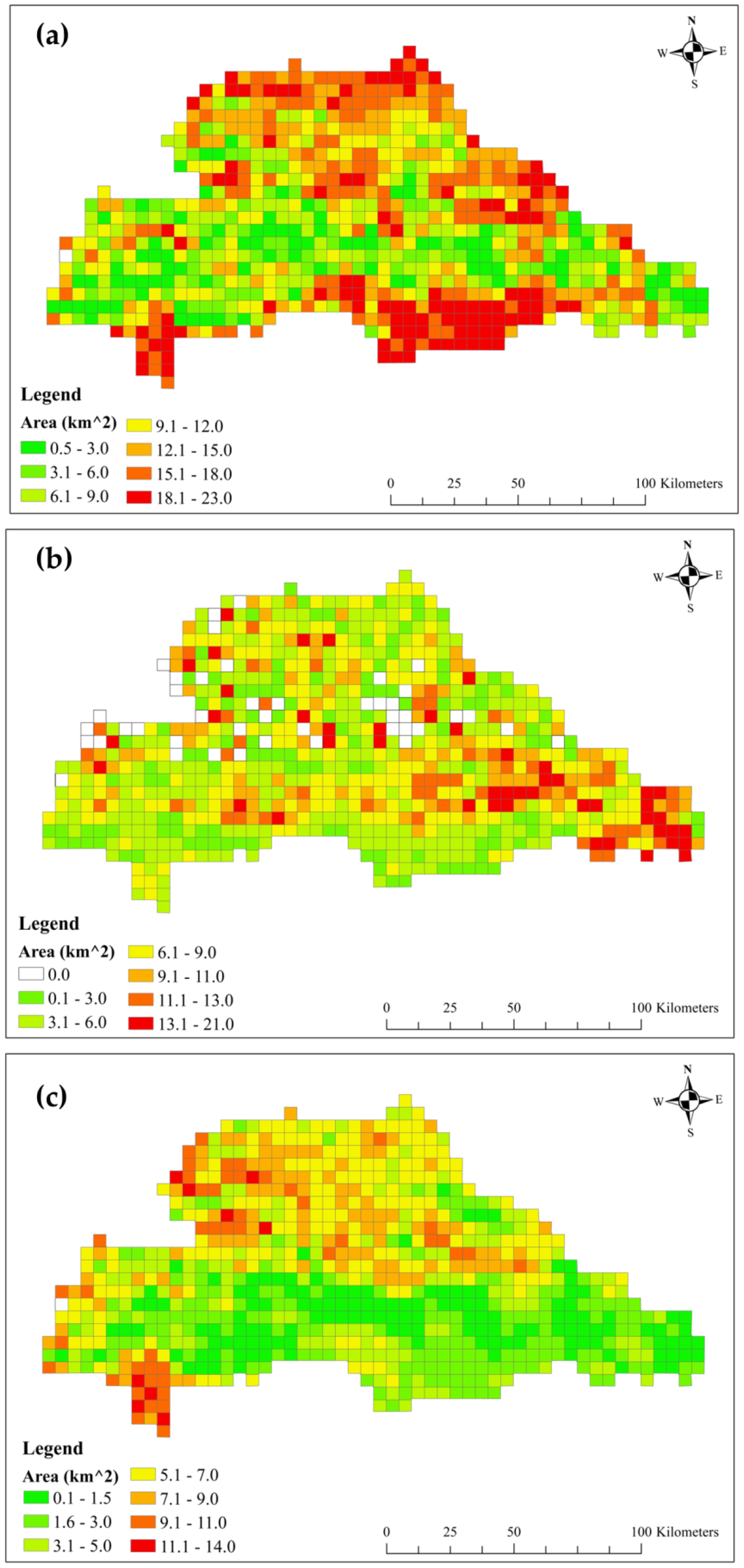
3.1. Paddy and Irrigated Dry Crops Area for Each Cell

The producers’ and users’ accuracies of the MODIS imagery for paddy classification were between 75% and 82% [27]. The estimated Kappa coefficient for paddy classification was 0.79, while the total accuracy was 82%. The crop classification map of the study area is presented in Figure 5. The LAI map of the study area is shown in Figure 6 to display the differences in vegetation distribution within the basin. Figure 5 shows that most of the agricultural area in the river basin is cultivated by paddy in Kharif and left fallow in Rabi. Some downstream areas are cultivated by paddy in Kharif and irrigated dry crops in Rabi. Additionally, a significant agricultural area was used for cultivating irrigated dry crops in both seasons (Figure 5). This classified map was further processed to estimate the paddy and irrigated dry crops area in each cell of the river basin.
Figure 7a presents the paddy area allocation in various model cells during the Kharif season. The paddy area in cells varies from 0.5 to 23 km2, with cells having more than 18 km2 under the paddy dominating the study area. Thus, there is intensive cultivation of the paddy during the Kharif season. Mostly, those cells are located around the boundaries of the river basin (Figure 7a). Figure 7b presents the irrigated dry crops area in each cell during the Kharif season. The area under irrigated dry crops in a cell varies from 0 to 22 km2, with most cells having less than 3 km2 under irrigated dry crops. The cells with high irrigated dry crops area (>11 km2) are significantly less, located just above the Durgapur barrage (Figure 7b). The paddy cultivation in the rabi season is negligible in the study area; hence, the area under paddy is considered zero in all cells. In the rabi season, irrigated dry crops, i.e., wheat, pulses, and oilseeds, are mainly cultivated. Figure 7c presents the cell-wise distribution of the irrigated dry crops. The maximum irrigated dry crop area in a cell is 13 km2, and such cells are primarily located in the upland area of the basin (Figure 7c). Figure 7b,c show that the irrigated dry crops are cultivated over a larger area in the Kharif season than in the rabi season.

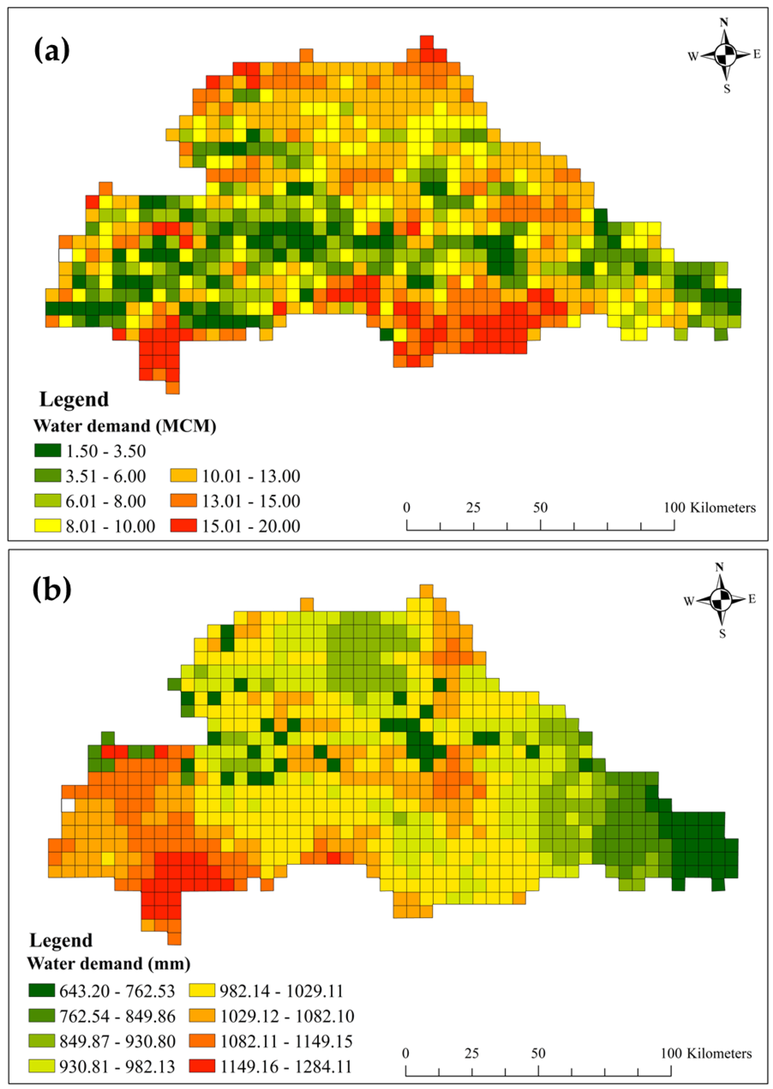
3.2. Temporal and Spatial Variation of Irrigation Demand in the Cell

The irrigated demand is estimated under two moisture deficit scenarios: zero allowable moisture depletion (AMD-0) and 50% allowable moisture depletion (AMD-50). Figure 8 presents the temporal variation of irrigation water demand under the AMD-0 and AMD-50 scenarios for one year (2015–2016) in a typical cell. The AMD-0 scenario means that the moisture or water level is not allowed to decrease, so the water demand is calculated daily to maintain the moisture or water level at 100%. Figure 8 shows that the module simulated the water demand every day, except when precipitation exceeded the crop evapotranspiration and percolation losses. In the cell, the Kharif water demand is higher than the Rabi because of the smaller agricultural area cultivated in the rabi season. The maximum irrigation demand in the cell occurred in the first week of June because of the delayed monsoon in 2015–2016. The AMD-50 means moisture or the water level is not allowed to decrease beyond 50%, so the water demand is calculated after 50% moisture or water level depletion. In this scenario, the water demand appeared after every 5 to 7 days in the rabi season. However, the time between two water demands appearance in the Kharif season varied depending on the rainfall contribution. The maximum irrigation demand occurred in the second week of August when the water demand for paddy and irrigated dry crops coincided.
The spatial distribution of irrigation demand (1 July 2015) for AMD-0 and AMD-50 scenarios is shown in Figure 9. Since July falls under the monsoon period, most cells receive rainfall on the day. However, the climatic variables (P, Tmax, Tmin) vary throughout the study area, so there is an uneven distribution of irrigation demand. The cells with no rainfall show higher irrigation demands (Figure 9a), while cells with rainfall depth exceeding the ETc have no irrigation demand, even under AMD-0 conditions. The rest of the cells show low to medium irrigation demands. Under the AMD-50 scenario, most cells have no water demand because the water level and soil moisture are not depleted to 50% (Figure 9b). The soil moisture or water level is reduced beyond 50% in cells with water demands. However, the irrigation demand in those cells is more compared to the AMD-0 scenario, because the demands refer to cumulative demands of up to 50% moisture and water level depletion. A river basin’s water resources can be effectively managed using this knowledge of the temporal and spatial variations in the study area.

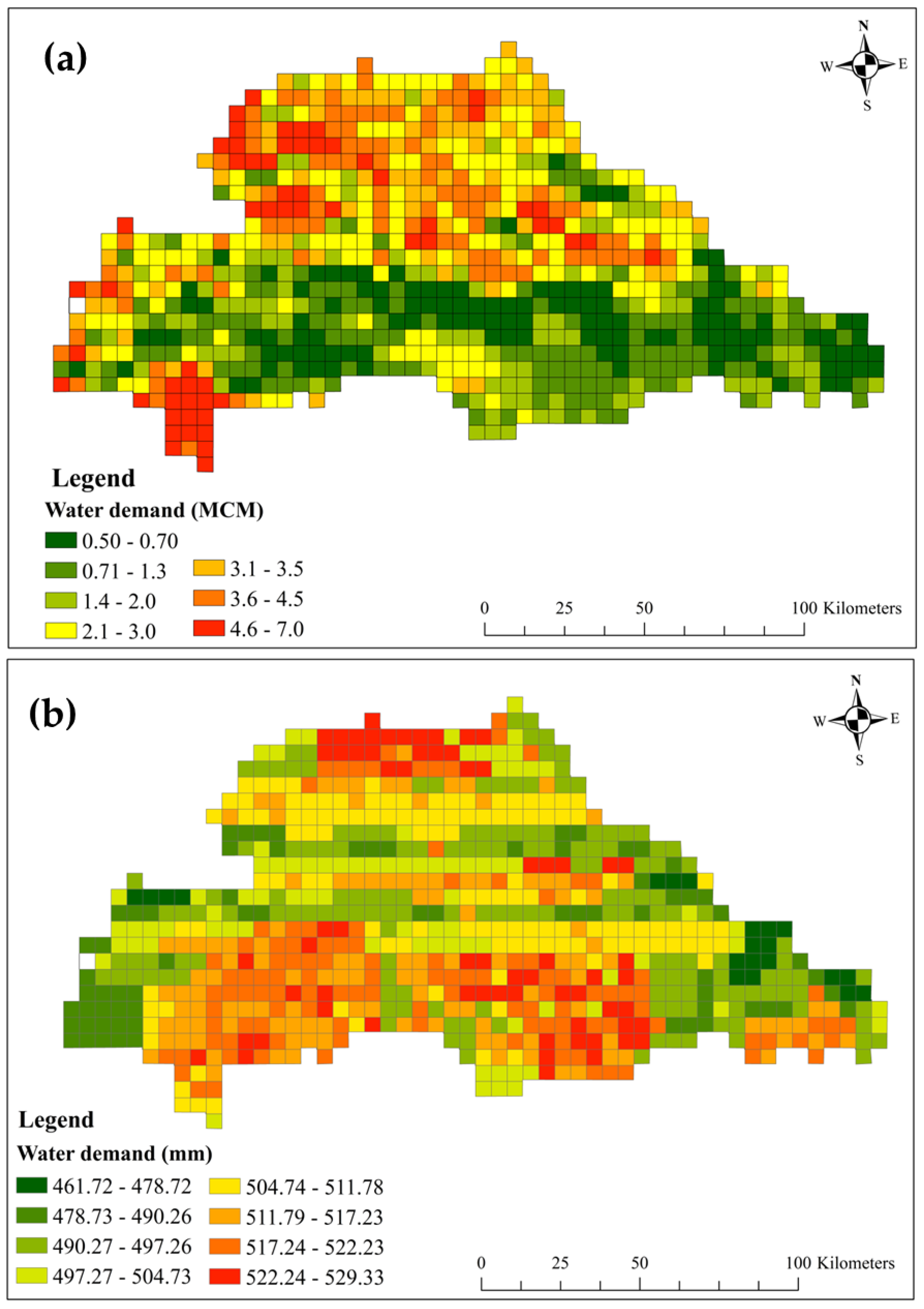
3.3. Kharif and Rabi Irrigation Demands

Figure 10 and Figure 11 present the Kharif and Rabi irrigation demands for the entire basin during 2009–2018 under AMD-0 and AMD-50 scenarios. In both scenarios, the Kharif irrigation demands varied annually because of the seasonal monsoon rainfall variability, affecting water demand. In India, the Kharif season mostly depends upon monsoon rainfall, and 70% of the annual rain falls within the Kharif season. However, irrigation demands in the rabi season did not vary significantly over ten years because of no or less rainfall in the rabi season. Figure 10 and Figure 11 show that the highest irrigation demand in the Kharif occurred in the 2015–2016 season under both scenarios compared to other years. If we compare the Kharif irrigation demands under both scenarios, it is higher in the AMD-0 scenario than in the AMD-50 scenario (Figure 10 and Figure 11). However, the rabi irrigation demand is only marginally more in the AMD-0 scenario. The annual irrigation demands (Kharif + Rabi) under AMD-0 and AMD-50 scenarios are presented in Table 1. From Table 1, it is evident that annual irrigation demand under the AMD-50 scenario is significantly less compared to the AMD-0 scenario. The maximum difference between the annual irrigation demands of the two scenarios occurred for the 2013–2014 year, whereas the minimum difference occurred in the 2015–2016 year. The yearly average irrigation demand under the AMD-50 scenario is 1966 MCM less than the annual irrigation demands under the AMD-0 scenario. Therefore, the AMD-50 scenario of irrigation demand estimation is a good approach for effective water management in a river basin.
The spatial variation of irrigation demand under the AMD-50 scenario in the Kharif and Rabi seasons (in volumetric (MCM) and linear (mm) units) is presented in Figure 12a–d. From Figure 12 and Figure 13, it is evident that there are differences in the spatial variation of irrigation demands between the volumetric and linear units. This is mainly due to the spatial variation of agricultural area in the river basin. The Kharif irrigation demand varies from 1.5 to 20 MCM (Figure 12a) and 643 to 1285 mm (Figure 12b). The Kharif irrigation demand in MCM is highest (15 to 20 MCM) in the cells around the basin’s boundary. This is due to the intensive agriculture around the basin’s boundary (Figure 7a). The Kharif irrigation demand was lowest, mainly at the center and downstream of the basin in both units, where the forest and urban areas are present. The rabi irrigation demand varied over the basin, with a maximum demand of 7.0 MCM or 530 mm and minimum demand of 0.5 MCM or 461 mm (Figure 13a,c). The cells with higher irrigation demand in the rabi season are located in upland areas of the basin, where the irrigated dry crops are primarily cultivated in the rabi season (Figure 7c). The low irrigation demands occurred in the lowland areas of the basin where the cultivation of irrigated dry crops is low.

4. Discussion

A satellited-based hydrological model, NHM-I, was developed for assessing the distributed water resources in the entire land mass of India. Paul et al. [14] developed the ROU module and implemented it in the NHM-I module, along with other modules. They also tested the developed model in Kabini catchment area, India, and found satisfactory results. Paul et al. [40] tested the credibility of the NHM-I model in the Subarnarekha river basin, India, using a robust hierarchical operational testing scheme. They concluded that the NHM-I model is geographically and climatically transposable with satisfactory results. Paul et al. [41] compared the performance of the NHM-I model with the SWAT model in Baitarini river basin, India, and concluded that the NHM-I model performed better than the SWAT model, especially in estimating the annual peak flows. From the above discussion, we can say that the NHM-I model has great potential in simulating the hydrological processes.
In this study, a water demand module was developed for the NHM-I model to simulate the irrigation demands based on soil moisture deficits. The classified MODIS imageries reasonably estimated paddy and irrigated dry crops area in each cell in Kharif and Rabi seasons. Most of the river basin’s agricultural area falls under the rice-fallow class (paddy in Kharif and fallow in Rabi). Kumar et al. [42] reported that West Bengal and Jharkhand states have 3.18 Mha of the area under the rice-fallow class. Similarly, Gumma et al. [43] reported that the 3.34 Mha area of West Bengal and Jharkhand states belong to the rice-fallow class. As the river basin lies in West Bengal and Jharkhand states, we can say that our findings are consistent with the above studies’ findings. The important finding of this study is that intensive paddy cultivation is done mostly at the basin boundary in the Kharif season, whereas irrigated dry crops are mostly cultivated in upland areas in the Rabi season. These findings are consistent with West Bengal and Jharkhand states’ district statistics.
The NHM-I model, with its new water demand module, can effectively simulate irrigation demands using remote sensing input data. Fries et al. [44] and Khan et al. [45] used a similar approach to estimate irrigation demands based on soil moisture deficits and crop water requirements. However, these studies are model-independent and lack a hydrological approach in estimating the soil moisture deficits, therefore, the irrigation demands. An assessment of irrigation demands in AMD-0 and AMD-50 conditions revealed that the irrigation demand frequency under the AMD-50 condition is less spatial and temporary; however, the magnitude of irrigation demand is higher than in the AMD-0 conditions. It is due to the AMD-50 scenario consideration of cumulative demand up to 50% moisture or water level depletion as irrigation demand. The above findings are consistent with the studies of Fries et al. [44] and Khan et al. [45]. The seasonal analysis of irrigation demands disclosed that irrigation demands varied annually in Kharif but not significantly in Rabi. This is due to the monsoon rainfall variability in the Kharif season. The same was reported in the studies of Prasanna [46], Kumar et al. [47], and Pradhan et al. [48]. The spatial analysis of Kharif and Rabi irrigation demands reveals that the cells near the basin’s boundary have the highest Kharif irrigation demand due to extensive paddy cultivation. At the same time, the upland areas of the basin have the highest irrigation demand during the rabi season. The difference between the annual irrigation demands under the AMD-0 and AMD-50 scenarios is high, with an average value of 1966 MCM of water. That means if the water management officials and farmers follow the AMD-50 scenario for supplying or managing the irrigation water, an average of 1966 MCM can be saved in the basin. The saved water can be stored and utilized correctly to cultivate irrigated dry crops in fallow areas of the Rabi season.
The developed water demand module is robust and fast and requires less data. The integrated NHM-I model can assess the spatial and temporal dynamics of soil moisture and irrigation demands. The allowable moisture or water level depletions are prescribed by the user. Therefore, the user can assess the irrigation demands under different scenarios. This will be helpful in effective water management. The classified MODIS imageries accurately classify paddy and irrigated dry crops. However, more ground control points from the extensive field survey can further enhance the classification accuracy. Only one soil moisture zone is considered in the water balance equation of the NHM-I model. Considering multiple soil moisture zones instead of one will significantly enhance the accuracy of the water demand module and the NHM-I model. In the estimation of ETc, only standard conditions are considered using the Kc factor and are not considered ETc under stressful soil moisture conditions. Additionally, the capillary rise from groundwater is not accounted for in the soil moisture balance. Apart from the above limitations, the NHM-I with water demand module offers a practical approach to assess the irrigation demands spatially and temporarily.

5. Conclusions

Assessment of irrigation demands is necessary for effective water management in a river basin. This study assessed spatial and temporal variations of irrigation demands by integrating a new water demand module with the NHM-I model. This study concludes that the NHM-I model with a water demand module has great potential for simulating the irrigation demands with remote sensing input data. In the study area, irrigation demands in Kharif varied annually, and high irrigation demands were observed at basin boundaries and upstream areas. In the basin, an average of 1966 MCM of water can be saved per year using the AMD-50 scenario compared to the AMD-0 scenario. This analysis will help the water management officials and farmers to effectively manage basin water for irrigation.
Classifying the paddy and irrigated dry crops from the remote sensing data is difficult, as it requires high-resolution cloud-free imageries and more ground control points. The classified MODIS imageries from ICRISAT reasonably estimated the area under paddy and irrigated dry crops. Due to data restrictions, this study considered only two crop classes (paddy and irrigated dry crops). Future work may consider more crop classes in the analysis to know the variation of irrigation demands. This water demand module can be tested in other reservoir command areas to enhance its credibility. Additionally, this analysis can be expanded to the whole landmass of India, as the NHM-I model is built for the entirety of India. However, this expansion faces challenges regarding the availability of classified agricultural maps of the entire India. The crop classification in the whole of India from remote sensing imageries is a rigorous task to do. Handling these data with other spatial and temporal data will also become challenging, as it requires high-performance computers and a database. However, increasing computational power and emerging machine-learning techniques can be laid as a platform for this progressive work to be done in the future.

Author Contributions

Conceptualization, K.S. and R.S.; methodology, K.S., A.B. and A.M.; software, K.S. and A.B.; validation, K.S. and A.B.; formal analysis, K.S.; investigation, R.S. and A.M.; data curation, K.S. and A.B.; writing—original draft preparation, K.S.; writing—review and editing, R.S. and A.M.; visualization, K.S., R.S. and A.M.; supervision, R.S. and A.M.; project administration, R.S.; funding acquisition, R.S. All authors have read and agreed to the published version of the manuscript.

Funding

This research was funded by the National Institute of Hydrology (NIH), Roorkee, under the National Hydrology Project (Grant number: NHP/IIT Kharagpur/NIH-2018).

Data Availability Statement

The data presented in this study are available on request from the corresponding author. The data are not publicly available due to project embargo reasons.

Acknowledgments

The authors thank the National Institute of Hydrology (NIH), Roorkee, for their financial support during this study. The technical assistance of Partha Pratim Samanta in developing and implementing the reservoir module is thankfully recognised.

Conflicts of Interest

The authors declare no conflict of interest.

References

  1. De-Wrachien, D.; Schultz, B.; Goli, M.B. Impacts of population growth and climate change on food production and irrigation and drainage needs: A world-wide view. Irrig. Drain. 2021, 70, 981–995. [Google Scholar] [CrossRef]
  2. Nazemi, A.; Wheater, H.S. On inclusion of water resource management in Earth system models–Part 1: Problem definition and representation of water demand. Hydrol. Earth Syst. Sci. 2015, 19, 33–61. [Google Scholar] [CrossRef] [Green Version]
  3. Sushanth, K.; Mishra, A.; Mukhopadhyay, P.; Singh, R. Real-time streamflow forecasting in a reservoir-regulated river basin using explainable machine learning and conceptual reservoir module. Sci. Total Environ. 2023, 861, 160680. [Google Scholar] [CrossRef]
  4. Torres-Rua, A.F.; Ticlavilca, A.M.; Bachour, R.; McKee, M. Estimation of Surface Soil Moisture in Irrigated Lands by Assimilation of Landsat Vegetation Indices, Surface Energy Balance Products, and Relevance Vector Machines. Water 2016, 8, 167. [Google Scholar] [CrossRef] [Green Version]
  5. Zhang, D.; Zhou, G. Estimation of soil moisture from optical and thermal remote sensing: A review. Sensors 2016, 16, 1308. [Google Scholar] [CrossRef] [Green Version]
  6. Babaeian, E.; Sadeghi, M.; Jones, S.B.; Montzka, C.; Vereecken, H.; Tuller, M. Ground, proximal, and satellite remote sensing of soil moisture. Rev. Geophys. 2019, 57, 530–616. [Google Scholar] [CrossRef] [Green Version]
  7. De-Lima, R.S.; Li, K.Y.; Vain, A.; Lang, M.; Bergamo, T.F.; Kokamägi, K.; Burnside, N.G.; Ward, R.D.; Sepp, K. The Potential of Optical UAS Data for Predicting Surface Soil Moisture in a Peatland across Time and Sites. Remote Sens. 2022, 14, 2334. [Google Scholar] [CrossRef]
  8. Li, Z.L.; Leng, P.; Zhou, C.; Chen, K.S.; Zhou, F.C.; Shang, G.F. Soil moisture retrieval from remote sensing measurements: Current knowledge and directions for the future. Earth Sci. Rev. 2021, 218, 103673. [Google Scholar] [CrossRef]
  9. Choi, M.; Jacobs, J.M.; Bosch, D.D. Remote sensing observatory validation of surface soil moisture using Advanced Microwave Scanning Radiometer E, Common Land Model, and ground based data: Case study in SMEX03 Little River Region, Georgia, US. Water Resour. Res. 2008, 44, W08421. [Google Scholar] [CrossRef] [Green Version]
  10. Manfreda, S.; Brocca, L.; Moramarco, T.; Melone, F.; Sheffield, J. A physically based approach for the estimation of root-zone soil moisture from surface measurements. Hydrol. Earth Syst. Sci. 2014, 18, 1199–1212. [Google Scholar] [CrossRef] [Green Version]
  11. Stefan, V.G.; Indrio, G.; Escorihuela, M.J.; Quintana-Seguí, P.; Villar, J.M. High-Resolution SMAP-Derived Root-Zone Soil Moisture Using an Exponential Filter Model Calibrated per Land Cover Type. Remote Sens. 2021, 13, 1112. [Google Scholar] [CrossRef]
  12. Zhuo, L.; Han, D. The relevance of soil moisture by remote sensing and hydrological modelling. Procedia Eng. 2016, 154, 1368–1375. [Google Scholar] [CrossRef] [Green Version]
  13. Jung, G.; Wagner, S.; Kunstmann, H. Joint climate–hydrology modelling: An impact study for the data-sparse environment of the Volta Basin in West Africa. Hydrol. Res. 2012, 43, 231–248. [Google Scholar] [CrossRef]
  14. Paul, P.K.; Kumari, N.; Panigrahi, N.; Mishra, A.; Singh, R. Implementation of cell-to-cell routing scheme in a large scale conceptual hydrological model. Environ. Model. Softw. 2018, 101, 23–33. [Google Scholar] [CrossRef]
  15. Gaur, S.; Bandyopadhyay, A.; Singh, R. From changing environment to changing extremes: Exploring the future streamflow and associated uncertainties through integrated modelling system. Water Resour. Manag. 2021, 35, 1889–1911. [Google Scholar] [CrossRef]
  16. Bathurst, J.C.; O’connell, P.E. Future of distributed modelling: The Systeme Hydrologique Europeen. Hydrol. Process. 1992, 6, 265–277. [Google Scholar] [CrossRef]
  17. Haddeland, I.; Lettenmaier, D.P.; Skaugen, T. Effects of irrigation on the water and energy balances of the Colorado and Mekong river basins. J. Hydrol. 2006, 324, 210–223. [Google Scholar] [CrossRef]
  18. Biemans, H.; Haddeland, I.; Kabat, P.; Ludwig, F.; Hutjes, R.W.A.; Heinke, J.; Von Bloh, W.; Gerten, D. Impact of reservoirs on river discharge and irrigation water supply during the 20th century. Water Resour. Res. 2011, 47, W03509. [Google Scholar] [CrossRef] [Green Version]
  19. Wu, Y.; Chen, J. Estimating irrigation water demand using an improved method and optimizing reservoir operation for water supply and hydropower generation: A case study of the Xinfengjiang reservoir in southern China. Agric. Water Manag. 2013, 116, 110–121. [Google Scholar] [CrossRef]
  20. Wada, Y.; Wisser, D.; Bierkens, M.P. Global modeling of withdrawal, allocation and consumptive use of surface water and groundwater resources. Earth Syst. Dyn. 2014, 5, 15–40. [Google Scholar] [CrossRef] [Green Version]
  21. Brunner, M.I.; Gurung, A.B.; Zappa, M.; Zekollari, H.; Farinotti, D.; Stähli, M. Present and future water scarcity in Switzerland: Potential for alleviation through reservoirs and lakes. Sci. Total Environ. 2019, 666, 1033–1047. [Google Scholar] [CrossRef]
  22. Gorguner, M.; Kavvas, M.L. Modelling impacts of future climate change on reservoir storages and irrigation water demands in a Mediterranean basin. Sci. Total Environ. 2020, 748, 141246. [Google Scholar] [CrossRef]
  23. Zhang, P.; Ma, W.; Hou, L.; Liu, F.; Zhang, Q. Study on the Spatial and Temporal Distribution of Irrigation Water Requirements for Major Crops in Shandong Province. Water 2022, 14, 1051. [Google Scholar] [CrossRef]
  24. Mainuddin, M.; Kirby, M.; Chowdhury, R.A.R.; Shah-Newaz, S.M. Spatial and temporal variations of, and the impact of climate change on, the dry season crop irrigation requirements in Bangladesh. Irrig. Sci. 2015, 33, 107–120. [Google Scholar] [CrossRef]
  25. Christou, A.; Dalias, P.; Neocleous, D. Spatial and temporal variations in evapotranspiration and net water requirements of typical Mediterranean crops on the island of Cyprus. J. Agric. Sci. 2017, 155, 1311–1323. [Google Scholar] [CrossRef]
  26. Wu, D.; Fang, S.; Li, X.; He, D.; Zhu, Y.; Yang, Z.; Xu, J.; Wu, Y. Spatial-temporal variation in irrigation water requirement for the winter wheat-summer maize rotation system since the 1980s on the North China Plain. Agric. Water Manag. 2019, 214, 78–86. [Google Scholar] [CrossRef]
  27. Gumma, M.K.; Thenkabail, P.S.; Teluguntla, P.; Rao, M.N.; Mohammed, I.A.; Whitbread, A.M. Mapping rice-fallow cropland areas for short-season grain legumes intensification in South Asia using MODIS 250 m time-series data. Int. J. Digit. Earth 2016, 9, 981–1003. [Google Scholar] [CrossRef] [Green Version]
  28. Kumari, N.; Srivastava, A.; Sahoo, B.; Raghuwanshi, N.S.; Bretreger, D. Identification of suitable hydrological models for streamflow assessment in the Kangsabati River Basin, India, by using different model selection scores. Nat. Resour. Res. 2021, 30, 4187–4205. [Google Scholar] [CrossRef]
  29. Liang, X.; Lettenmaier, D.P.; Wood, E.F.; Burges, S.J. A simple hydrologically based model of land surface water and energy fluxes for general circulation models. J. Geophys. Res. Atmos. 1994, 99, 14415–14428. [Google Scholar] [CrossRef]
  30. Arnold, J.G.; Srinivasan, R.; Muttiah, R.S.; Williams, J.R. Large area hydrologic modeling and assessment Part I: Model development. J. Am. Water Resour. Assoc. 1998, 34, 73–89. [Google Scholar] [CrossRef]
  31. Wijesekara, G.N.; Gupta, A.; Valeo, C.; Hasbani, J.G.; Qiao, Y.; Delaney, P.; Marceau, D.J. Assessing the impact of future land-use changes on hydrological processes in the Elbow River watershed in southern Alberta, Canada. J. Hydrol. 2012, 412, 220–232. [Google Scholar] [CrossRef]
  32. Feldman, A. Hydrologic Modeling System HEC-HMS; Technical Reference Manual; US Army Corps of Engineeres: Washington, DC, USA, 2000; Available online: https://www.hec.usace.army.mil/software/hec-hms/documentation/HEC-HMS_Technical%20Reference%20Manual_(CPD-74B).pdf (accessed on 1 December 2022).
  33. Sieber, J.; Purkey, D. WEAP: Water Evaluation and Planning System; User Guide; Technical Report; Stockholm Environment Institute, U.S. Center: Somerville, MA, USA, 2015; Available online: https://www.weap21.org/downloads/WEAP_User_Guide.pdf (accessed on 1 December 2022).
  34. Ruiz, L.; Varma, M.R.; Kumar, M.M.; Sekhar, M. Water balance modelling in a tropical watershed under deciduous forest (Mule Hole, India): Regolith matric storage buffers the groundwater recharge process. J. Hydrol. 2010, 380, 460–472. [Google Scholar] [CrossRef] [Green Version]
  35. Sekhar, M.; Ruiz, L. Groundwater flow modeling of Gundal sub-basin in Kabini river basin, India. Asian J. Water Environ. Pollut. 2004, 1, 65–77. [Google Scholar]
  36. Raziei, T.; Pereira, L.S. Estimation of ETo with Hargreaves–Samani and FAO-PM temperature methods for a wide range of climates in Iran. Agric. Water Manag. 2013, 121, 1–18. [Google Scholar] [CrossRef]
  37. Valiantzas, J.D. Temperature-and humidity-based simplified Penman’s ET0 formulae. Comparisons with temperature-based Hargreaves-Samani and other methodologies. Agric. Water Manag. 2018, 208, 326–334. [Google Scholar] [CrossRef]
  38. Hargreaves, G.H.; Samani, Z.A. Reference crop evapotranspiration from temperature. Appl. Eng. Agric. 1985, 1, 96–99. [Google Scholar] [CrossRef]
  39. Chapagain, A.K.; Hoekstra, A.Y. The blue, green and grey water footprint of rice from production and consumption perspectives. Ecol. Econ. 2011, 70, 749–758. [Google Scholar] [CrossRef]
  40. Paul, P.K.; Gaur, S.; Kumari, B.; Panigrahy, N.; Mishra, A.; Singh, R. Diagnosing credibility of a large-scale conceptual hydrological model in simulating streamflow. J. Hydrol. Eng. 2019, 24, 04019004. [Google Scholar] [CrossRef]
  41. Paul, P.K.; Zhang, Y.; Mishra, A.; Panigrahy, N.; Singh, R. Comparative Study of Two State-of-the-Art Semi-Distributed Hydrological Models. Water 2019, 11, 871. [Google Scholar] [CrossRef] [Green Version]
  42. Kumar, R.; Mishra, J.S.; Upadhyay, P.K.; Hans, H. Rice fallows in the Eastern India: Problems and prospects. Indian J. Agric. Sci. 2019, 89, 567–577. [Google Scholar] [CrossRef]
  43. Gumma, M.K.; Thenkabail, P.S.; Teluguntla, P.; Whitbread, A.M. Monitoring of spatiotemporal dynamics of Rabi rice fallows in south Asia using remote sensing. In Geospatial Technologies in Land Resources Mapping, Monitoring and Management; Springer: Cham, Switzerland, 2018; pp. 425–449. [Google Scholar] [CrossRef]
  44. Fries, A.; Silva, K.; Pucha-Cofrep, F.; Oñate-Valdivieso, F.; Ochoa-Cueva, P. Water balance and soil moisture deficit of different vegetation units under semiarid conditions in the andes of southern Ecuador. Climate 2020, 8, 30. [Google Scholar] [CrossRef] [Green Version]
  45. Khan, S.; Rasool, A.; Irshad, S.; Hafeez, M.B.; Ali, M.; Saddique, M.; Asif, M.; Hasnain, Z.; Naseem, S.; Alwahibi, M.S.; et al. Potential soil moisture deficit: A useful approach to save water with enhanced growth and productivity of wheat crop. J. Water Clim. Chang. 2021, 12, 2515–2525. [Google Scholar] [CrossRef]
  46. Prasanna, V. Impact of monsoon rainfall on the total foodgrain yield over India. J. Earth Syst. Sci. 2014, 123, 1129–1145. [Google Scholar] [CrossRef]
  47. Kumar, H.V.; Shivamurthy, M.; Lunagaria, M.M. Impact of rainfall variability and trend on rice yield in coastal Karnataka. J. Agrometeorol. 2017, 19, 286–287. [Google Scholar] [CrossRef]
  48. Pradhan, A.; Chandrakar, T.; Nag, S.K.; Dixit, A.; Mukherjee, S.C. Crop planning based on rainfall variability for Bastar region of Chhattisgarh, India. J. Agrometeorol. 2020, 22, 509–517. [Google Scholar] [CrossRef]
Figure 1. Damodar river basin.
Remotesensing 15 01119 g001
Figure 2. A framework of the national hydrological model—India (NHM-I).
Remotesensing 15 01119 g002
Figure 3. Conceptual representation of irrigation water demand estimation.
Remotesensing 15 01119 g003
Figure 4. Conceptual representation of distributed approach for estimating irrigation demand.
Remotesensing 15 01119 g004
Figure 5. Crop classification map of the study area.
Remotesensing 15 01119 g005
Figure 6. LAI map of the study area.
Remotesensing 15 01119 g006
Figure 7. (a) Paddy area, (b) irrigated dry cops area in each cell for the Kharif season, (c) irrigated dry cops area in each cell for the Rabi season.
Remotesensing 15 01119 g007
Figure 8. Irrigation water demand in a typical cell for one-year under AMD-0 and AMD-50 scenarios.
Remotesensing 15 01119 g008
Figure 9. Spatial variation of irrigation water demand under (a) AMD-0 and (b) AMD-50.
Remotesensing 15 01119 g009
Figure 10. Yearly irrigation water demand of the Kharif and Rabi (AMD-0).
Remotesensing 15 01119 g010
Figure 11. Yearly irrigation water demand of the Kharif and Rabi (AMD-50).
Remotesensing 15 01119 g011
Figure 12. Spatial variation of irrigation demand in the Kharif season in (a) MCM and (b) mm of 2015–2016.
Remotesensing 15 01119 g012
Figure 13. Spatial variation of irrigation demand in the Rabi season in (a) MCM and (b) mm of 2015–2016.
Remotesensing 15 01119 g013
Table 1. Annual irrigation demand under AMD-0 and AMD-50 scenarios.
YearAnnual Irrigation Demand (MCM)Difference (MCM)
AMD-0AMD-50
2009–201010,254.858086.282168.57
2010–201110,186.088269.721916.36
2011–20129302.147708.731593.41
2012–20139665.427689.891975.53
2013–20148889.036344.412544.63
2014–20159932.787871.162061.63
2015–201610,583.448923.321660.12
2016–20179147.147189.301957.84
2017–201810,596.708778.341818.36
Disclaimer/Publisher’s Note: The statements, opinions and data contained in all publications are solely those of the individual author(s) and contributor(s) and not of MDPI and/or the editor(s). MDPI and/or the editor(s) disclaim responsibility for any injury to people or property resulting from any ideas, methods, instructions or products referred to in the content.

