A Transfer-Based Framework for Underwater Target Detection from Hyperspectral Imagery

Abstract

The detection of underwater targets through hyperspectral imagery is a relatively novel topic as the assumption of target background independence is no longer valid, making it difficult to directly detect underwater targets using land target information. Meanwhile, deep-learning-based methods have faced challenges regarding the availability of training datasets, especially in underwater conditions. To solve these problems, a transfer-based framework is proposed in this paper, which exploits synthetic data to train deep-learning models and transfers them to real-world applications. However, the transfer becomes challenging due to the imparity in the distribution between real and synthetic data. To address this dilemma, the proposed framework, named the transfer-based underwater target detection framework (TUTDF), first divides the domains using the depth information, then trains models for different domains and develops an adaptive module to determine which model to use. Meanwhile, a spatial–spectral process is applied prior to detection, which is devoted to eliminating the adverse influence of background noise. Since there is no publicly available hyperspectral underwater target dataset, most of the existing methods only run on simulated data; therefore, we conducted expensive experiments to obtain datasets with accurate depths and use them for validation. Extensive experiments verify the effectiveness and efficiency of TUTDF in comparison with traditional methods.

1. Introduction

Hyperspectral imagery (HSI) contains data in the form of a cube containing two spatial dimensions and one spectral dimension. Unlike RGB images, which only contain three bands, each pixel in HSI has rich spectral information, which usually possesses hundreds of immediately adjacent bands. Generally, the reflection spectrum of a material is called its spectral signature, which could be used to distinguish this from others. Thus, HSI is widely exploited in various fields, such as agricultural management, resource exploration, and military detection. Research on HSI usually includes dimensionality reduction [1], target detection [2,3] and classification [4], among which hyperspectral target detection (HTD) is a significant part. This can be divided into object-level and pixel-level detection. Object-level detection [5] is the detection of a specific target object as a whole, and existing methods tend to detect this target by extracting spatial–spectral features and using RGB image object-detection algorithms. However, pixel-level detection is more mainstream. This is usually regarded as a binary classifier that can be used to determine whether the pixel belongs to the target or background [6]. To be more precise, differing from the binary classifier, it performs a classification by assigning each pixel to one of two classes: the detector used to perform HTD finds an appropriate threshold, which corresponds to a boundary between the class of target absence and the class of target presence [4]. Generally, detectors fall into three categories according to whether their background information and target spectral information are known. In the first category, neither is available—for example, RX [7], which merely detects anomalies with limited performance. The target information is known in the second group, while the background information is unknown, as in CEM [8]. As for the third category, such as OSP [9], both the target and background information are known.

In general, the spectral signature can directly reflect the type of substance; there seems to be no need to learn and classify them using a network. However, when the target is submerged and the situation is not the same, the signature of the to-be-detected target will change due to interference from the water background. Compared with land-based HTD, less research has been conducted on underwater target detection (UTD) from HSI. There are challenges in the direct application of land-based methods to UTD, mainly because the observed target spectra, i.e., water-leaving radiance, are highly dependent on the inherent optical properties (IOPs) of water and the depth of the target, making it difficult to distinguish the target from the background. In response, research [6,10,11] may provide partial solutions. According to the implementation scene, these solutions fall into one of two categories.

In the first category, which we shall call the underwater scene, a spectral imager is attached to an autonomous underwater vehicle, which directly dives underwater to acquire HSI. A rapid target detection technique employing band selection (BS) is proposed [10]. This first uses a constrained target optimal refraction factor band selection (CTOIFBS) method to choose bands with high levels of information and low band correlation. Then, an underwater spectral imaging system incorporating the optimal subset of wavebands is built for underwater target picture capture. To detect the desired underwater targets, the CEM algorithm is finally employed. This overcomes the problems of a complex background and poor imaging environment. However, the expenses associated with underwater vehicle photography are considerable, the range of movement is limited, and BS loses a lot of spectral information while increasing its speed.

In the second category, denoted a satellite remote sensing (SRS) scene, the pipeline generally starts with IOPs estimation due to the water body’s influence on the off-water irradiance. IOPs are calculated using mathematical optimization methods (such as SOMA [12]), then a target space is constructed based on a bathymetric model to solve the issue of missing depth information, and finally, detection is carried out using a manifold learning method [11]. However, manifold learning has the drawback of being time-consuming. Deep learning has also been applied to address this issue. A network named IOPE-Net [13], in the form of an unsupervised autoencoder, was proposed to estimate IOPs and achieved a good performance. In light of this, a self-improving framework [6] is proposed, which is based on deep learning and EM theory. Firstly, anomalies are detected by a joint anomaly detector with a high threshold to obtain a guide training set, which is used to train a depth estimation network. Then, shallower pixels are screened as targets and used to train a detection network. After that, the guide training set is updated based on the detection results. Two networks are alternately iterated to boost the final detection performance. Although this framework shows a large improvement in detection performance compared to several land-based methods, it requires different iterations; thus, the issue of it being time-consuming remains, and the initial guided training set often leads to few-shot problems in practice due to its small size.

To facilitate the experiment, this paper focuses on unmanned aerial vehicle remote sensing (UAVRS) scenarios, which have the advantages of a low cost, broad applicability, high spatial resolution, and good real-time performance. In fact, in both UAVRS and SRS scenarios, underwater targets are detected from the air, so the proposed method can also be extended to SRS scenarios.

Based on the above scenarios, we propose a new framework for underwater target detection, which does not require repeated iterations or time-consuming mathematical optimization operations. We can quickly perform detection after training a model with the a priori land information of the target and the HSI of the specific water area. Deep learning methods are used throughout the pipeline. Since there is no publicly accessible HSI dataset containing underwater targets, and the received spectra are strongly influenced by the water body, which varies from water to water, it is difficult to generalize the model even if a dataset is available. Therefore, we used synthetic data to train the model for each specific water area. To solve the adaptation problem from the source domain to the target domain, we adopted domain randomization and domain adaptation strategies. Meanwhile, the spatial–spectrum process was used to utilize spatial information.

Generally speaking, the proposed framework consists of three main phrases: synthetic data, domain selection, and target detection. Firstly, we used a specific network to estimate the water quality parameters, combined the information of the target to plot the spectral distance variation curve with depth, and found the depth maximum where the spectral distance shows almost no change. Then, we selected certain target pixels, water background pixels, and depths to synthesize the underwater target observation spectra based on the bathymetric model and divided them into different domains according to depth intervals. Then, we used synthetic data and proper water background data to train the target detection network and domain prediction network. After that, we fine-tuned the detection network’s fully connected layers, i.e., the domain adaptive sub-network, according to domains. Finally, the trained model can be directly used for detection.

Aiming to quickly detect underwater targets, our main idea is to use synthetic data for training and directly apply them to real-world tasks. The closer the real-world data are to the domain of the synthetic data, the corresponding model of that domain will lead to better detection results.

In summary, the major contributions of our work are listed as follows:

• A novel framework named TUTDF has been proposed to address the underwater detection problem based on deep learning and synthetic data theory. To the best of our knowledge, this is the first time that synthetic data have been used to train models, then directly applied to underwater target detection tasks in real environments.
• We propose a synthetic data approach based on depth interval partitioning to solve the transfer problem from the synthetic data source domain to the real data target domain. We also develop domain prediction and domain adaptive networks to select the corresponding sourced domain model to yield more accurate detection results.
• Due to the lack of hyperspectral underwater target datasets, we conducted extensive experiments to obtain realistic underwater target datasets. As far as we know, this is the first hyperspectral underwater target dataset with accurate depth information.

The remainder of this paper is structured as follows. Section 2 first introduces the relevant model, followed by a detailed description of the experimental procedure and some theory, before finally displaying the proposed method in more detail. The experimental results are shown in Section 3. Some of the components are discussed in Section 4. In Section 5, we summarize the entire work and draw a comprehensive conclusion.

2. Materials and Methods

In this section, a brief review of the bathymetric model of ocean hyperspectral data is given, providing a fundamental field background. The experimental implementation will be presented, which describes the data acquisition and processing in more detail. Then, some theories are introduced, and our proposed method is described in detail. Finally, the evaluation criteria, data partitioning, and other experimental details are described.

2.1. Bathymetric Model

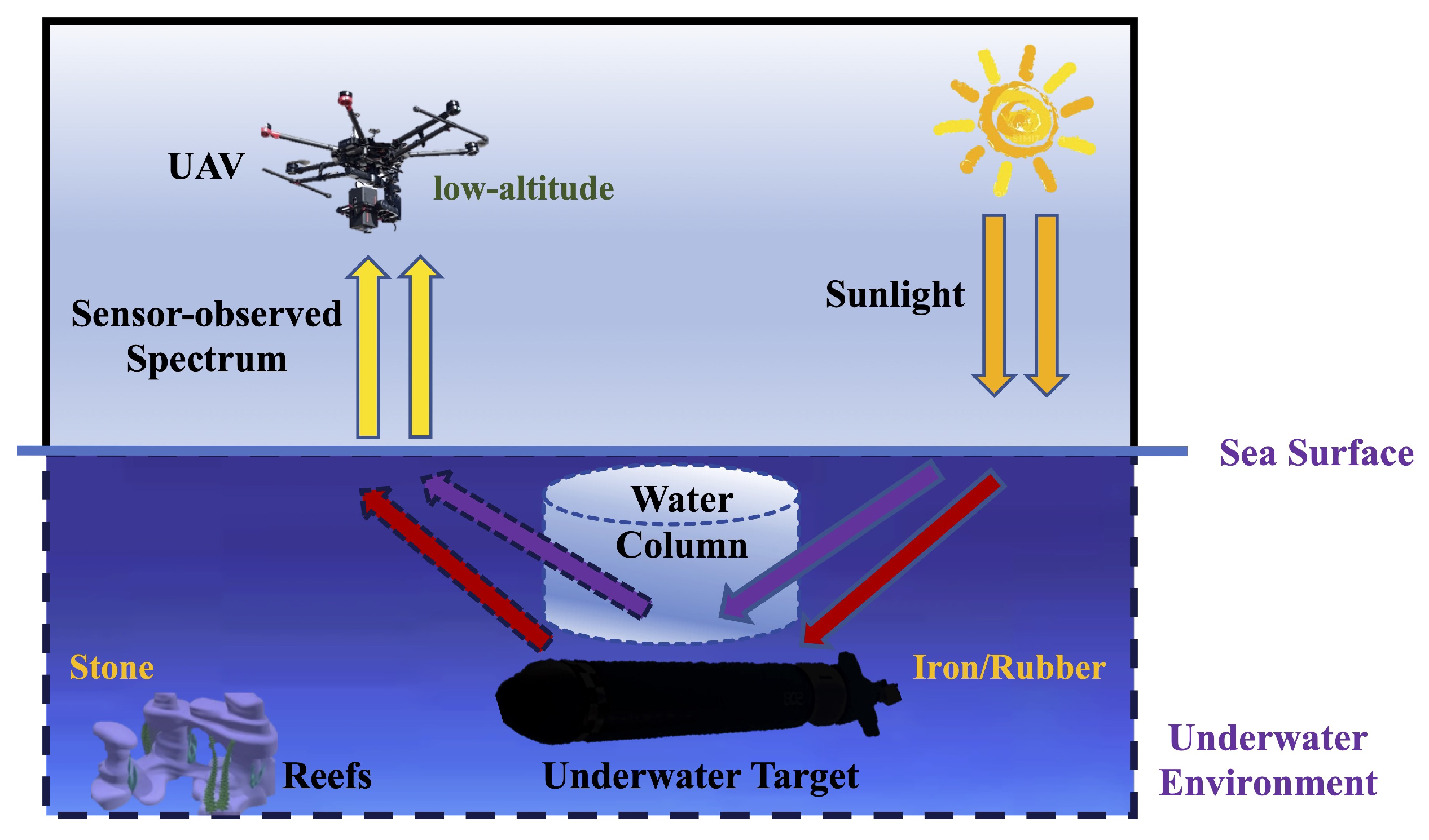
Generally, the observed spectrum for a submerged target received by a sensor can be described as a specific equation, which is called the bathymetric model [14]. This can be formulated as Equation (1). The process described by the formula is illustrated in Figure 1. Sunlight entered the water body and was reflected by the water column or the underwater targets. The reflected rays were transmitted from the water column and received by the sensor. In addition to atmospheric attenuation, there is a large amount of light attenuation in the water, with increasing depth. The water surface may suffer from weak polarization when reflecting sunlight. For convenience, as other researchers have, we ignored the effects of the water–air interface, which can be represented by the empirical relation of Lee et al. [15]. Therefore, the target spectrum received by the sensor is affected by the following: the upper surface of the target, water quality, depth, and sunlight intensity and angle.

$$\mathbf{r}\left(\lambda \right)={\mathbf{r}}_{\infty }\left(\lambda \right)\left(1-{\mathrm{e}}^{-\left({\mathbf{k}}_d\left(\lambda \right)+{\mathbf{k}}_u^c\left(\lambda \right)\right)H}\right)+{\mathbf{r}}_B\left(\lambda \right){\mathrm{e}}^{-\left({\mathbf{k}}_d\left(\lambda \right)+{\mathbf{k}}_u^b\left(\lambda \right)\right)H}$$

(1)

where $\lambda$ is the wavelength, $\mathbf{r}\left(\lambda \right)$ is the off-water reflectance, ${\mathbf{r}}_{\infty }\left(\lambda \right)$ is the reflectance of the “optical deep water” [16], ${\mathbf{r}}_B\left(\lambda \right)$ is the reflectance of the target to be detected as the priori information, ${\mathbf{k}}_d\left(\lambda \right)$ is the downward attenuation coefficient of the light in the water, ${\mathbf{k}}_u^c\left(\lambda \right)$ and ${\mathbf{k}}_u^b\left(\lambda \right)$ are the upward attenuation coefficients of the water column and target, respectively, and H is the depth information of the underwater target.

Further, ${\mathbf{r}}_{\infty }\left(\lambda \right)$, ${\mathbf{k}}_d\left(\lambda \right)$, ${\mathbf{k}}_u^c\left(\lambda \right)$ and ${\mathbf{k}}_u^b\left(\lambda \right)$ are determined by the IOPs of water: absorption coefficient $\mathbf{a}\left(\lambda \right)$, backscattering coefficient ${\mathbf{b}}_b\left(\lambda \right)$. In addition, in remote sensing, ${\mathbf{k}}_d\left(\lambda \right)$ is also related to the solar zenith angle $\theta$. The commonly referred-to water properties’ estimation is the estimate $\mathbf{a}\left(\lambda \right)$, ${\mathbf{b}}_b\left(\lambda \right)$ from the hyperspectral image of the water surface. In this paper, we used an unsupervised water properties estimation network IOPE-Net in the form of an autoencoder to estimate $\mathbf{a}\left(\lambda \right)$, ${\mathbf{b}}_b\left(\lambda \right)$. The relationship between the above parameters is as follows:

$$\mathbf{k}\left(\lambda \right)=\mathbf{a}\left(\lambda \right)+{\mathbf{b}}_b\left(\lambda \right)$$

(2)

$$\mathbf{u}\left(\lambda \right)={\mathbf{b}}_b\left(\lambda \right)/(\mathbf{a}\left(\lambda \right)+{\mathbf{b}}_b\left(\lambda \right))$$

(3)

$${\mathbf{k}}_d\left(\lambda \right)=\mathbf{k}\left(\lambda \right)/cos\left(\theta \right)$$

(4)

$${\mathbf{k}}_u^c\left(\lambda \right)=1.03\times {(1+2.4\mathbf{u}\left(\lambda \right))}^{0.5\mathbf{k}\left(\lambda \right)}$$

(5)

$${\mathbf{k}}_u^b\left(\lambda \right)=1.04\times {(1+5.4\mathbf{u}\left(\lambda \right))}^{0.5\mathbf{k}\left(\lambda \right)}$$

(6)

2.2. Experimental Implementation

Due to the novelty of hyperspectral underwater target detection, there is no publicly available dataset containing underwater targets; therefore, much of the existing work is based on simulated data, which is not a good way to check the effectiveness of the method in real environments, and applications in real environments often have more issues to consider. Therefore, we conducted extensive and effective experiments to obtain a real underwater target dataset and selected some data for validation.

In this section, we conducted an outdoor UAV experiment and an indoor pool experiment. Some preliminary conclusions were obtained from the UAV experiment. After a simplification of some influencing parameters, the indoor pool experiment was used to obtain a dataset with accurate depths.

2.2.1. Outdoor UAV Experiment

The UAV experiment was conducted in the outdoor swimming pool of Northwestern Polytechnical University (34.01°N, 108.45°E, 11:00–12:00, 17 January 2023). We first shot the underwater targets with UAV to form a basis for subsequent indoor experiments with precise depth. A brief description of the outdoor UAV experiment process and preliminary conclusions is as follows.

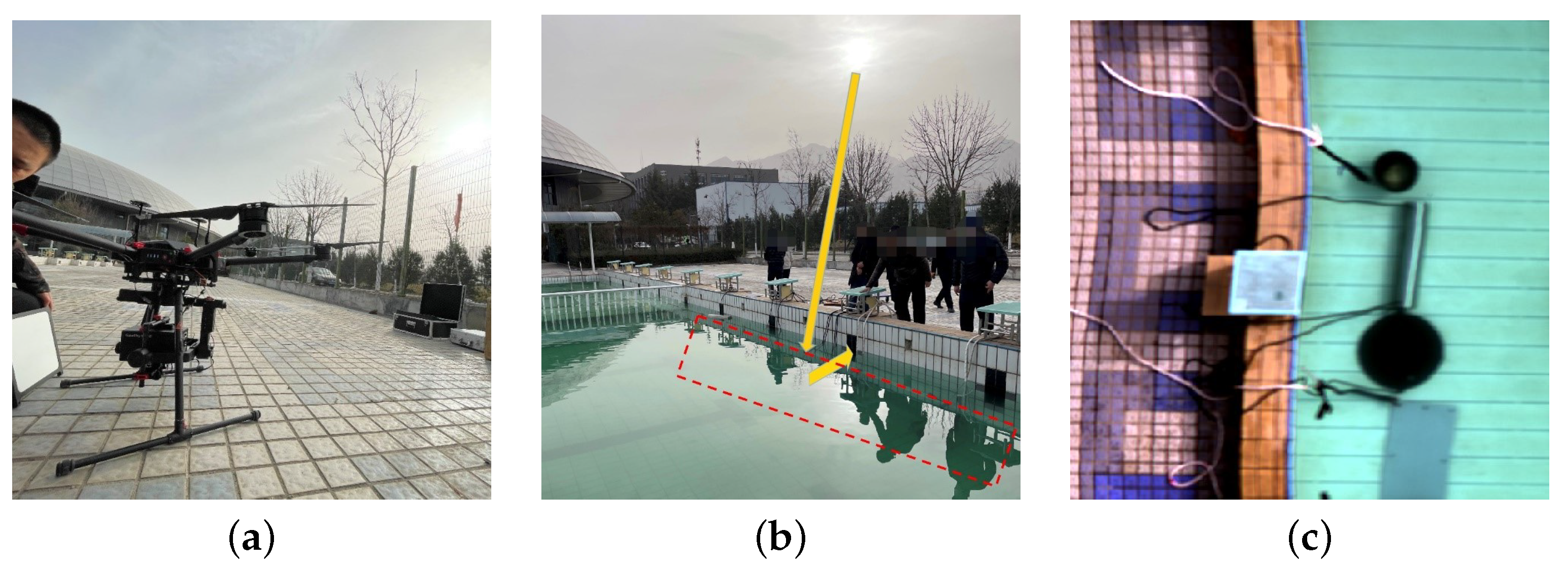
(1) Equipment and materials: The Gaia Sky-mini3 unmanned airborne hyperspectrometer is mainly designed for outdoor or long-range imaging tests of larger objects and has some applications that require portable operation. Gaia Sky-mini3 has a spectral range of 400–1000 nm, a spectral resolution of 5.5 nm and a spatial resolution of 1024 × 448. Then, we used DJI M600 PRO UAV, which has a vertical hovering accuracy of 0.5 m, to carry the spectrometer for the pool experiment, as shown in Figure 2a.

As exhibited in Figure 2b, we selected iron, rubber, and stone as underwater target materials of interest. Iron is the most common material for underwater vehicles, rubber is an anechoic material that is commonly used by underwater submarines to avoid sonar detection, and stone is a simulation of some underwater reefs. Detailed information on the targets is presented later in the indoor pool experiment 5.

(2) Data Acquisition: The UAV hovering vertical water surface shooting. As shown in Figure 3b, when tilting a certain angle to shoot, especially when the angle receives a direct reflection of light from the water surface, it will be beyond the water surface polarization phenomenon, affecting the quality of photography. As shown in Figure 3c, when looking at the pseudo-color image, a slight spatial distortion is clear, which is tolerable and does not affect its spectral profile. The detailed steps are as follows.

• step1: The reference board, which is usually called ‘white board’, was taken on the ground for reflectance correction and to fix the exposure time, as shown in Figure 3a. The shooting time, latitude and longitude were recorded for solar zenith angle calculation. The ‘gray cloth’ was laid flat on the ground. The lens cap was closed to obtain the ‘black board’ data.
• step2: The UAV flew to 20, 50, and 100 m altitudes to acquire images of the targets on the land. The ‘gray cloth’ was also taken at each altitude for atmospheric correction.
• step3: Targets were placed at 0.89 m in the pool. Another shot was taken of the ‘white board’ on the ground and the exposure time was fixed again. The UAV flew to 20, 50, and 100 m altitudes to capture target images underwater. The ‘gray cloth’ was taken at each altitude.
• step4: The data taken by the spectrometer were copied to the computer for processing. Using the software Spectral VIEW, atmospheric calibration was performed with “gray cloth” data, and automatic reflectance calibration was performed by selecting “whiteboard”, “blackboard” and raw data.

(3) Preliminary conclusion: Through an analysis of the obtained curves, we obtained the following preliminary conclusions and experiences. The spectral curve of the underwater target with a flat surface and uniform material does not significantly change with the change in shooting height; however, for the target with an uneven surface, with the increase in shooting height, pixel-mixing occurred and the curve of a point in the center of the surface may significantly change. An outdoor UAV needs to consider atmospheric attenuation, shooting angle, solar zenith angle, and distortion problems. Atmospheric attenuation occurred after shooting a gray cloth for atmospheric correction. The shooting angle was vertical water hovering shooting, avoiding the direct reflection of sunlight on the water’s surface. The solar zenith angle can be calculated based on latitude and longitude, as well as time.

Due to the limited depth of the pool, the water background is not ‘optically deep’, and the water quality cannot be effectively estimated. Moreover, it is difficult to obtain data for targets at different accurate depths. Therefore, we conducted the following indoor pool experiments.

2.2.2. Indoor Pool Experiment

In the anechoic pool laboratory of the College of Navigation, Northwestern Polytechnical University, there is a hydraulic lift rod, which can achieve depth variations from 0 to 3.1 m with an accuracy of 0.01 m. In addition, the pool water is deep and the indoor light is relatively weak, so the water background is optically deep. Here, we aimed to obtain underwater target data with an accurate depth.

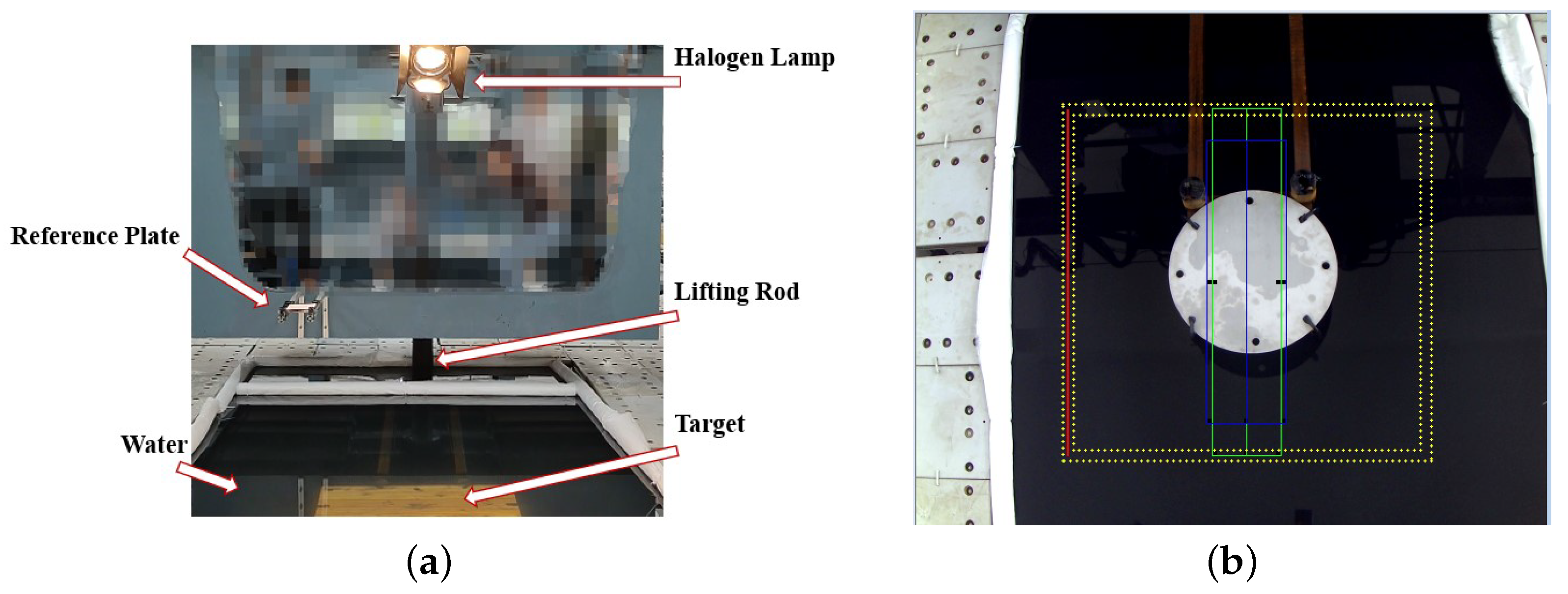
(1) Environment and materials: The experimental site is shown in Figure 4. Atmospheric attenuation can be ignored due to the close shooting distance. There was no significant direct sunlight indoors, and unlike outdoors, here, the ‘white board’ and target were placed horizontally and shot within the same image. That is, the light incident on the ‘white board’ and the water surface was the same. We used the data from the ‘white board’ for area calibration in the software Spectral VIEW. Therefore, the solar zenith angle was not considered here and was set to 0. The hyperspectral camera still shot vertically over the water’s surface. Depth, water quality, and target material were considered. The spatial resolution for the pool experiment scene was 1.72 mm, so the pixel mixing problem can be ignored. The difference between the light source for the outdoor and the indoor pool was the intensity of the sunlight, which affects the transmission depth of light in the water body and the detectable depth. Similarly, the water quality will also affect these parameters. Although there are some differences in light intensity and water quality, the transmission mechanism of these two was consistent; they fit the same bathymetric model (1) after calibration.

The experimental targets were fixed on the fabricated bracket, and the bracket near the targets was tied with black adhesive tape to reduce the interference of reflected light. As exhibited in Figure 5, iron and rubber plates had dimensions of 1 × 0.5 m, the disc’s diameter was 0.66 m, the cylinder’s length was 0.9 m, and the diameter was 0.2 m.

(2) Data Acquisition: In Figure 6, we used a bracket to hold the target horizontally, and the bracket was connected to a hydraulic lift rod to achieve depth variations from 0 to 3.1 m with an accuracy of 0.01 m. Gaia Field–V10 is a portable push-broom spectral imager with a spectral resolution of 2.8 nm, band range of 400–1000 nm, and spatial resolution of 658 × 696. The spectral imager was positioned 4.2 m directly above the target for vertical photography, at which point the spatial resolution was 1.72 mm. The ‘white board’ with a side length of 0.15 m was placed on the water surface next to the target and included in all measurements. The reflectance calibration was performed according to Equation (7).

$${\mathbf{Ref}}_{\mathrm{target}}\left(\lambda \right)=\frac{\mathbf{D}{\mathbf{N}}_{\mathrm{target}}\left(\lambda \right)-\mathbf{D}{\mathbf{N}}_{\mathrm{dark}}\left(\lambda \right)}{\mathbf{D}{\mathbf{N}}_{\mathrm{white}}\left(\lambda \right)-\mathbf{D}{\mathbf{N}}_{\mathrm{dark}}\left(\lambda \right)}{\mathbf{Ref}}_{\mathrm{white}}\left(\lambda \right)$$

(7)

where $\mathbf{DN}$ (digital number) is the original HSI pixel’s brightness value and recorded grayscale value of objects. ${\mathbf{DN}}_{\mathrm{target}\left(\lambda \right)}$ refers to the image brightness value of the object to be measured; ${\mathbf{DN}}_{\mathrm{dark}\left(\lambda \right)}$ refers to the noise generated by the spectral imager itself, which was captured by the spectral imager with the lens cover closed; ${\mathbf{DN}}_{\mathrm{white}\left(\lambda \right)}$ refers to the brightness value of the reference plate (commonly known as white plate); ${\mathbf{Ref}}_{\mathrm{white}\left(\lambda \right)}$ refers to the standard reflectance value of the ‘white board’, and a 99% reference plate was used indoors. ${\mathbf{DN}}_{\mathrm{target}\left(\lambda \right)}-{\mathbf{DN}}_{\mathrm{dark}\left(\lambda \right)}$ and ${\mathbf{DN}}_{\mathrm{white}\left(\lambda \right)}-{\mathbf{DN}}_{\mathrm{dark}\left(\lambda \right)}$ eliminated the noise in the spectral imager system. The implementation site is shown in Figure 6.

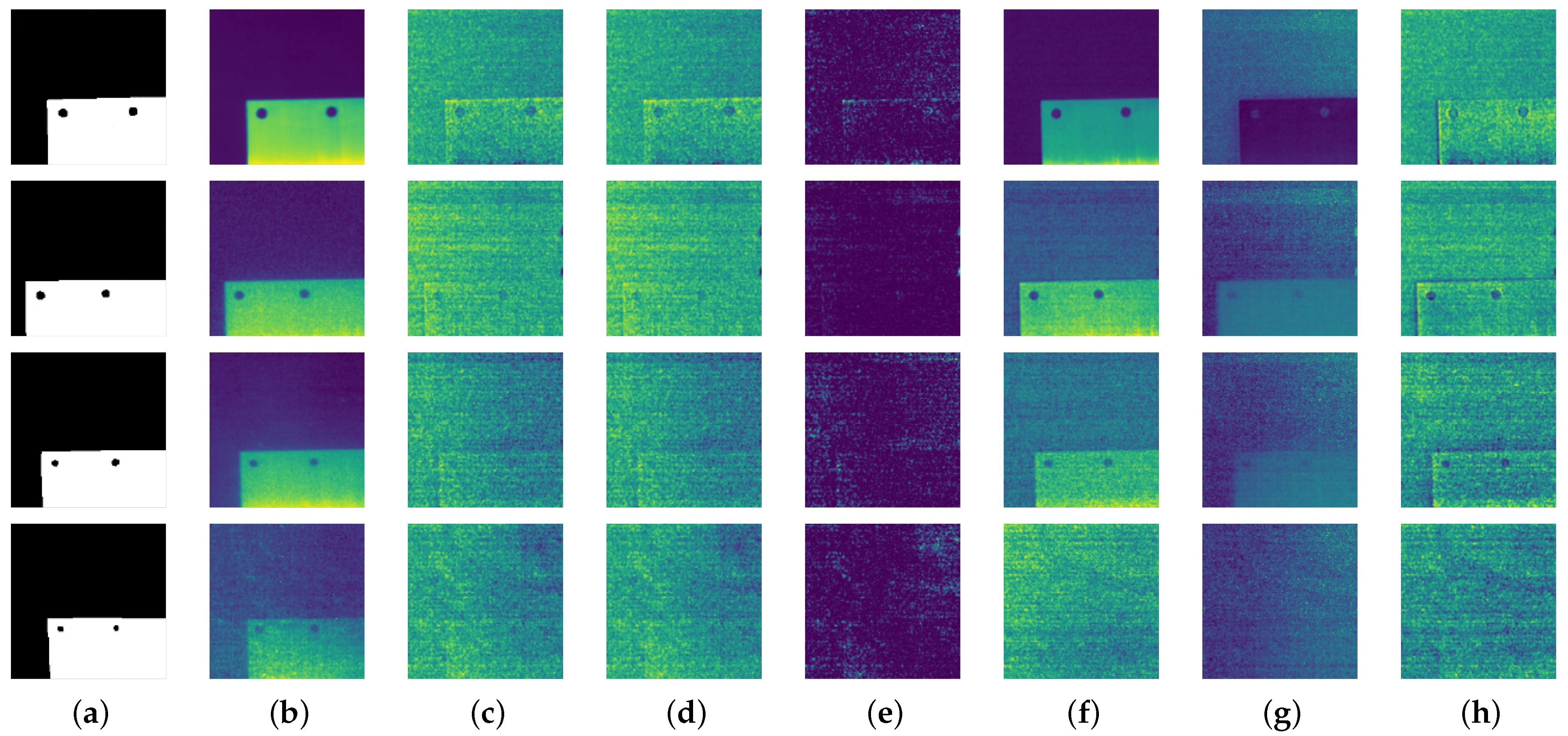
(3) Selection of Dataset Since the sunlight in the pool lab is weaker than that outdoors, we chose the depths of the human eye’s visual limit and, without a shadow, obscured a portion of the data for testing. As shown in Figure 7, they possessed 120 bands, from 400 to 780 nm. The HSI of the targets on the land was cropped at 10 × 10 pixels; water and the underwater targets had a shape of 100 × 100 after cropping. The pseudo-color pictures of the aforementioned data are as follows.

2.3. Related Theory

Many of the present artificial intelligence problems are attributed to insufficient data or available datasets being too small; even if it is relatively easy to obtain unlabeled data, the cost of manual labeling is often remarkably high. For the application of deep learning to hyperspectral underwater target detection tasks, especially low-altitude, fast detection tasks, there are unfortunately no corresponding publicly available datasets at present. Acquiring a large number of corresponding datasets is costly, which poses a significant challenge when training neural networks to perform detection tasks.

Synthetic data are a fundamental approach to solving the data problem [17], i.e., generating artificial data from scratch or using advanced data manipulation techniques to produce novel and diverse training examples, and have played a significant role in the field of computer vision and medical image processing. This paper generates synthetic data by partially “cutting” and model-based “pasting” with real data samples. Generally, the aim is to make the synthetic data as realistic as possible.

Synthetic data solve the problem of a lack of training sets. However, other problems arise. We refer to the training set generated from synthetic data as the source domain and the testing set obtained from the real world as the target domain. When we use the model trained from the source domain for target domain detection, the problem of domain transfer must be considered, i.e., how to ensure that the model from the source domain achieves good results in the target domain.

Inspired by the use of multi-path CNNs for the fine-grained recognition of cars [18] and the use of an attribute-guided feature-learning network for vehicle re-identification [19], we decided to divide multiple-source domains based on a fine-grained depth.

A multi-source domain adaptive task has multiple source domains and one target domain. The model learns from multiple source domains and applies what it has learned to predict the target domain. In general, this task seeks to identify the most useful source domain. Inspired by the domain-aware controller [20], we design a domain prediction network to select the source domain model that is to be applied to the target domain.

2.4. Proposed Method

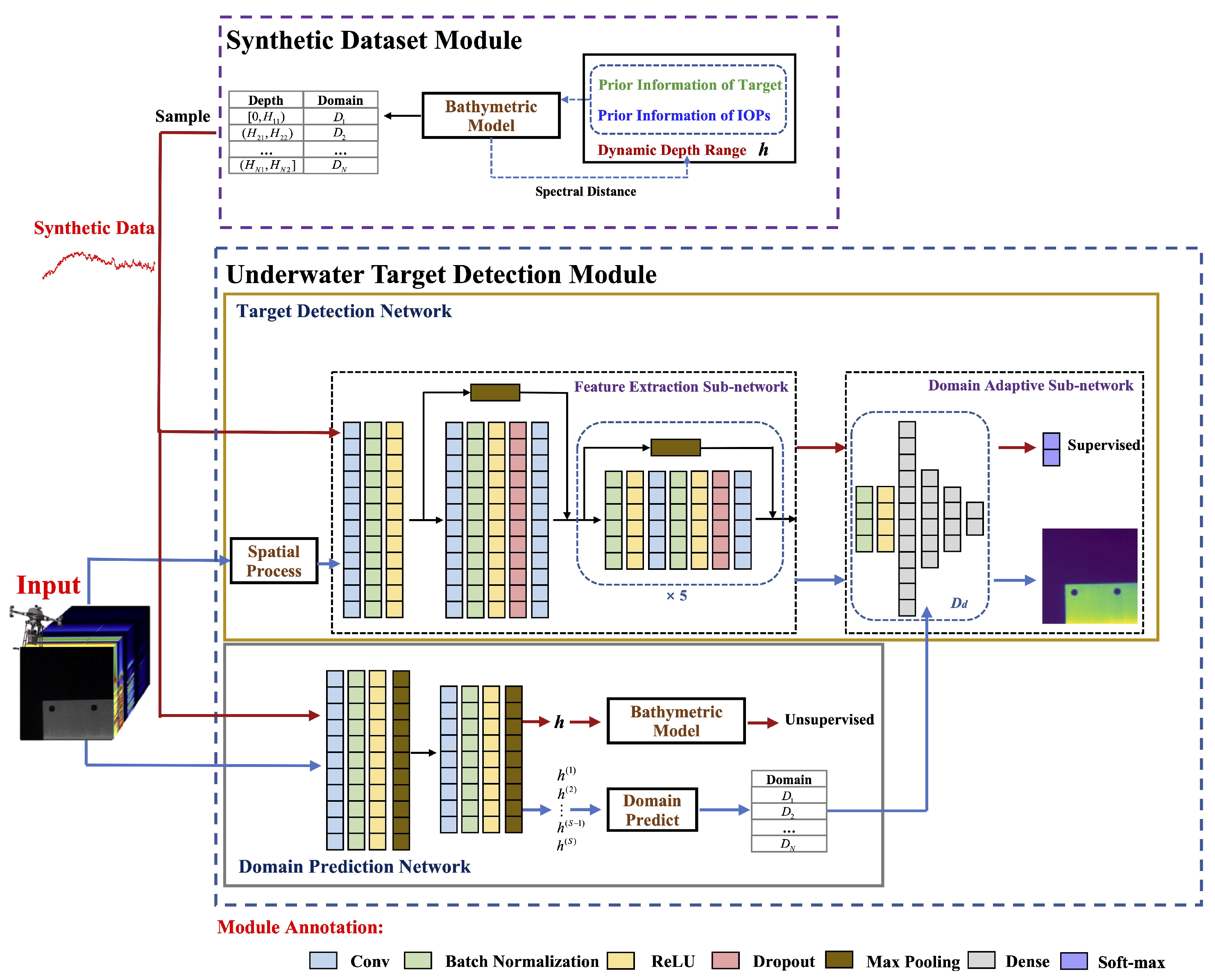
A Transfer-Based Underwater Target Detection Framework (TUTDF) is a deep-learning-based framework for hyperspectral underwater target detection, dedicated to fast detection with known a priori information about the target on-land. We address the lack of underwater target datasets by following the bathymetric model to synthesize data to yield training sets. We used an end-to-end network that does not require a rigorous upfront noise and dimensionality reduction effort for the backbone detection network. To solve the source-to-target domain adaptation problem, we set multiple source domains according to the depth range in the synthetic data module and designed a domain prediction network to select the corresponding source domain model for detection based on the depth information. In order to utilize more spatial information, we performed a spatial–spectral process before detection to improve the performance. All the contents are shown in Figure 8. TUTDF consists of two modules: a Synthetic Dataset Module and Underwater Target Detection Module.

The Synthetic Dataset Module is the initial part of TUTDF, which is used to create the training set for the target detection module. We set the depth range and divided different source domains according to the bathymetric model to generate a large amount of training data, which were used to sample and train the subsequent network.

The Underwater Target Detection Module is the most essential part of TUTDF, which consists of the target detection network and the domain prediction network. The following describes the overall flow of this module. The HSI to be detected is input to the target detection network after the spatial–spectral process. When training the synthetic datasets, the domain prediction network can ascertain the depth of each input pixel. According to the average depth value of some of the shallowest pixels, the corresponding domain adaptive sub-network is selected and combined with the feature extraction sub-network to form a complete target detection network, which is self-sufficient as it can use an under-fitted domain prediction network to estimate the depth information. We only need an approximate depth range to determine the corresponding source domain model.

2.5. Synthetic Dataset Module

Synthetic data should resemble real data more closely and cover all potential circumstances so that samples from the target domain are included in the source domains. Given the depth H, we may use Equation (8) to yield the underwater target reflectance ${\mathbf{r}}_{syn}\left(\lambda \right)$. Here, we adopted the simplified model [14], where ${\mathbf{k}}_c^c\left(\lambda \right)\approx {\mathbf{k}}_u^b\left(\lambda \right)$. Assuming that the noise in each HSI we used is $n\left(\lambda \right)$, we do not need to add extra noise during the synthesizing process.

$$\begin{array}{cc}\hfill {\mathbf{r}}_{syn}\left(\lambda \right)& =\left({\mathbf{r}}_{\infty }\left(\lambda \right)+\mathbf{n}\left(\lambda \right)\right)·\left(1-{\mathrm{e}}^{-\left({\mathbf{k}}_d\left(\lambda \right)+{\mathbf{k}}_u^c\left(\lambda \right)H\right.}\right)+\left({\mathbf{r}}_B\left(\lambda \right)+\mathbf{n}\left(\lambda \right)\right)·{\mathrm{e}}^{-\left({\mathbf{k}}_d\left(\lambda \right)+{\mathbf{k}}_u^b\left(\lambda \right)H\right.}\hfill \\ \hfill & ={\mathbf{r}}_{\infty }\left(\lambda \right)·\left(1-{\mathrm{e}}^{-\left({\mathbf{k}}_d\left(\lambda \right)+{\mathbf{k}}_u^c\left(\lambda \right)H\right.}\right)+{\mathbf{r}}_B\left(\lambda \right)·{\mathrm{e}}^{-\left({\mathbf{k}}_d\left(\lambda \right)+{\mathbf{k}}_u^b\left(\lambda \right)H\right.}+\hfill \\ \hfill & \mathbf{n}\left(\lambda \right)·\left(1+{\mathrm{e}}^{-\left({\mathbf{k}}_d\left(\lambda \right)+{\mathbf{k}}_u^b\left(\lambda \right)\right)H}-{\mathrm{e}}^{-\left({\mathbf{k}}_d\left(\lambda \right)+{\mathbf{k}}_u^c\left(\lambda \right)\right)H}\right)\hfill \\ \hfill & \approx {\mathbf{r}}_{\infty }\left(\lambda \right)·\left(1-{\mathrm{e}}^{-\left({\mathbf{k}}_d\left(\lambda \right)+{\mathbf{k}}_u^c\left(\lambda \right)\right)H}\right)+{\mathbf{r}}_B\left(\lambda \right)·{\mathrm{e}}^{-\left({\mathbf{k}}_d\left(\lambda \right)+{\mathbf{k}}_u^b\left(\lambda \right)\right)H}+\mathbf{n}\left(\lambda \right)\hfill \end{array}$$

(8)

We also need to consider H. The concept of spectral distance [21] is also relevant. Spectral distance describes the difference between two spectral vectors, calculated by treating the spectral curve as a spectral vector. The spectral distance d is defined in Equation (9), which represents the difference between ${\mathbf{r}}_B\left(\lambda \right)$ and ${\mathbf{r}}_{syn}\left(\lambda \right)$.

$$d=\sqrt{\sum {\left({\mathbf{r}}_{syn}\left(\lambda \right)-{\mathbf{r}}_B\left(\lambda \right)\right)}^2}$$

(9)

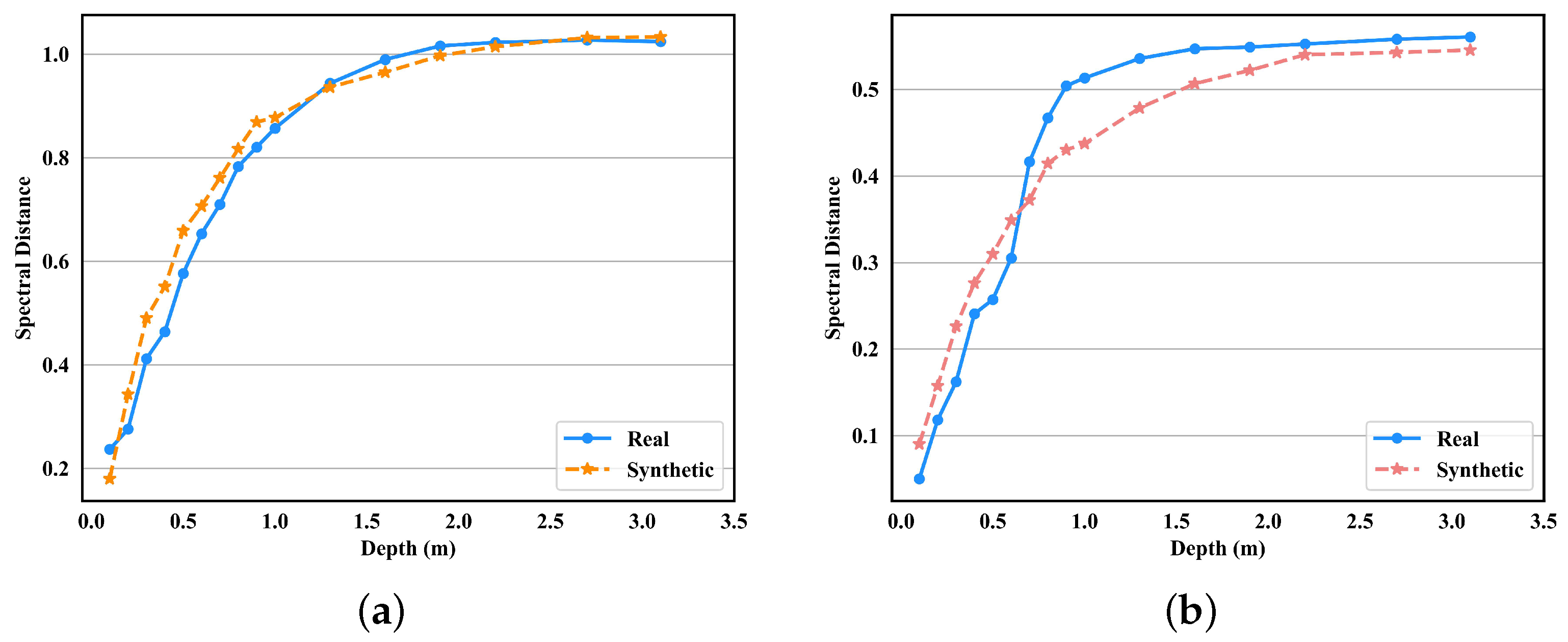
As shown in Figure 9, the spectral distance increases with depth, and the growth rate gradually decreases to zero. After reaching a particular depth, ${\mathbf{r}}_{syn}\left(\lambda \right)$ becomes the optical deep water ${\mathbf{r}}_{\infty }\left(\lambda \right)$, and the influence of the spectral imager resolution and noise renders the observed target spectrum indistinguishable from the water background. Therefore, the spectral distance curves of different materials were constructed under the specific water condition, with a maximum depth of $H_{deep}$.

A brief argument for the validity of using synthetic data is presented as follows. Firstly, the synthetic data are based on the model, which is reproducible and stable. Secondly, the spectral distance curves of the synthetic data match well with the real situation in Figure 9. Finally, the results regarding the real data in Section 4 will be more effective at proving the validity of the synthetic data.

As there are still differences between the real and synthetic spectra, they cannot be completely identical at all depths. As a result, it is expected that the distribution in the synthetic domain encompasses the real distribution. To this end, the depth interval $[0,H_{deep}]$ was divided into N overlapping sub-intervals, with the length of the interval being set to gradually increase from shallow to deep, as shown in Figure 10.

Each depth interval has M depths taken at equal intervals, and the data synthesized in different intervals belong to different domains $D_d,d=1,2,3,\dots ,N$. Figure 11 illustrates the whole process of synthesizing data, which is performed in the following steps.

• step1: Train a water quality estimation model $f_{IOP}(•)$ unsupervised with IOPE-Net from HSI of water areas.
• step2: Select P pixels from target donates ${\mathbf{r}}_B^i,i=1,2,3,\dots ,P$ and Q pixels from water donates ${\mathbf{r}}_{\infty }^j,j=1,2,3,\dots ,Q$. Calculate the water quality parameters $a^j\left(\lambda \right),b_b^j\left(\lambda \right)=f_{IOP}\left(r_{\infty }^j\left(\lambda \right)\right)$.
• step3: Use $\overline{{\mathbf{r}}_B^i\left(\lambda \right)}$ and $\overline{{\mathbf{r}}_{\infty }^j\left(\lambda \right)}$ to plot the spectral distance, combine the resolution conditions, set the maximum depth $H_{deep}$, divide into N overlapping sub-intervals, and select M depths at each sub-interval.
• step4: According to Equation (8), $P\times Q\times M$ underwater target samples are generated at each interval, and classified in domain $D_d$.
• step5: The pixels in domain $D_d$ and an equal number of optically deep water pixels are used as the training set for the domain adaptive sub-network. The data of N domains are used as the training set for the domain prediction network.

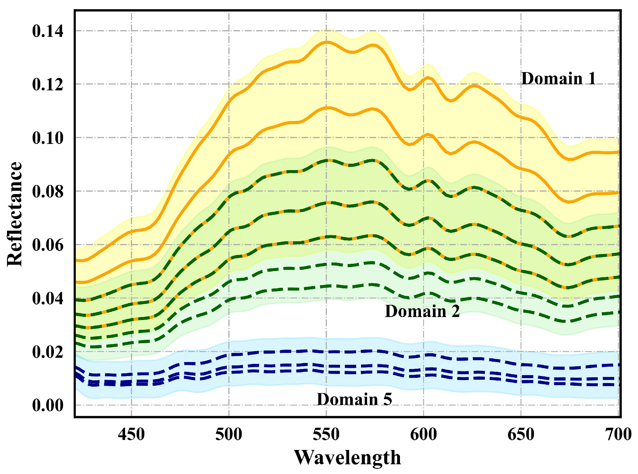
Figure 12 shows the results of partial synthesis data. In this case, we separately selected one pixel from iron and water. The reflectance decreases with increasing depth until ${\mathbf{r}}_{\infty }\left(\lambda \right)$, and there is an overlap between adjacent domains.

2.6. Target Detection Module

The module consists of two networks, the target detection network and the domain prediction network, described below.

2.6.1. Domain Predication Network

As can be seen from Figure 13, the first half of the network is a depth estimation network. During the training phase, the network employs unsupervised training in the form of an autoencoder. The input pixel is denoted by $\mathbf{x}$. Using a two-layer 1D-CNN encoder, the estimated depth $\widehat{h}$ is obtained. Then, we reconstructed the pixel $\widehat{\mathbf{x}}$ using $\widehat{h}$ and the bathymetric model in the decoder part. Finally, the network parameters were updated using the back-propagation of the loss function L.

$$L=L_{MSE}+{\lambda }_S{L}_S+{\lambda }_H{\parallel H\parallel }_2$$

(10)

$$L_{MSE}={\parallel x-\widehat{x}\parallel }_2$$

(11)

$$L_S=\frac{1}{\pi }arccos\frac{x·\widehat{x}}{{\parallel x\parallel }_2{\parallel \widehat{x}\parallel }_2}$$

(12)

where ${\parallel ·\parallel }_2$ is the $l_2$ norm of a given vector. $L_{MSE}$ is the mean square error loss function, describing the euclidean distance between x and $\widehat{x}$. $L_S$ is the spectral angle loss function, which describes the similarity in shape between x and $\widehat{x}$. ${\parallel H\parallel }_2$ is the depth-constraint loss function, which is a very important term in the loss function that keeps the estimated depth from being too large. ${\lambda }_S$ and ${\lambda }_H$ are the corresponding weighting coefficients of the loss function $L_{MSE}$ and ${\parallel H\parallel }_2$.

Since the depth estimate of the target is always small, we selected the smallest part of the depth value as the overall target depth. During the detection phase, the to-be-detected HSI is first fed into the depth estimation network to select the minimum S depths with a depth value of $h^{\left(s\right)}$; then, the depth values are processed by the domain prediction operation to select the model used in the domain adaptive network. The domain prediction operation is as follows.

$$\overline{h}=\frac{{\sum }_{s=1}^S{h}^{\left(s\right)}}{S}$$

(13)

The value of S was determined by considering the size of the target in the camera’s field of view. If the field of view is large and the target is small, the selected S is larger than the number of target points, which means that the estimated target depth will be large; thus, an inappropriate domain will be selected. If S is set too small, it may be disturbed by individual anomalies in the water background and estimate an inappropriate approximate overall target depth. Therefore, the setting of S can be expressed as follows.

$$S=N_{filed}\frac{S_{target}}{S_{filed}}$$

(14)

where $N_{filed}$ is the number of spatial pixels in the hyperspectral image captured by the camera, $S_{target}$ is the area determined by the target being detected (set to 1/4 of the area of the upper surface of the target being detected, as only a part of the target is captured), and $S_{filed}$ is the area of the field of view at a fixed shooting height.

For depth intervals of different domains, this setting ensures that no certain depth will occur at the boundary of the selected field.

$$D_d=\left\{\begin{array}{cc}{D}_1,& 0\le \overline{h}<\left(H_{12}+H_{21}\right)/2\\ D_2,& \left(H_{12}+H_{21}\right)/2\le \overline{h}<\left(H_{22}+H_{31}\right)/2\\ D_2,& \left(H_{12}+H_{21}\right)/2\le \overline{h}<\left(H_{22}+H_{31}\right)/2\\ \dots \\ D_N,& \left(H_{(N-1)2}+H_{N1}\right)/2\le \overline{h}<N\end{array}\right.$$

(15)

2.6.2. Target Detection Network

The network input is a pixel, i.e., a hyperspectral curve, which is regarded as a sequence input, and the output is the probability of the target to be detected. Two sub-networks comprise the target detection network: feature extraction sub-network and domain adaptive sub-network, as seen in Figure 14.

The feature extraction network is a generic backbone network. Recently, a specific deep network [22] successfully applied to long sequence data (ambulatory electrocardiograms) detection and classification. Inspired by that, we use a fully convolutional deep neural network as the backbone feature extraction network to achieve high performance without extra preprocessing (noise reduction, dimensionality reduction). The network simply inputs the original spectral sequence and generates the feature map through multilayer 1-D CNN with residual connectivity.

With a pixel $\mathbf{x}={\left\{x_i\right\}}_{i=1}^B$ containing B bands, for the feature extraction network, the output of the first block is:

$${\mathbf{y}}^{\left(1\right)}=h\left({\mathbf{w}}^{\left(1\right)}\ast \mathbf{x}+{\mathbf{b}}^{\left(1\right)}\right)$$

(16)

the output of the second block is:

$$\left\{\begin{array}{c}{\mathbf{y}}^{(2,1)}=h\left({\mathbf{w}}^{(2,1)}\ast {\mathbf{y}}^{\left(1\right)}+{\mathbf{b}}^{(2,1)}\right)\hfill \\ {\mathbf{y}}^{(2,2)}={\mathbf{w}}^{(2,2)}\ast {\mathbf{y}}^{(2,1)}+{\mathbf{b}}^{(2,2)}\hfill \\ {\mathbf{y}}^{\left(2\right)}={\mathbf{y}}^{(2,2)}\oplus {\mathbf{y}}^{\left(1\right)}\hfill \end{array}\right.$$

(17)

and the outputs of the successor blocks are:

$$\left\{\begin{array}{cc}\hfill {\mathbf{y}}^{(t,1)}& ={\mathbf{w}}^{(t,1)}\ast h\left({\mathbf{y}}^{(t-1)}\right)+{\mathbf{b}}^{(t,1)},\hfill \\ \hfill {\mathbf{y}}^{(t,2)}& ={\mathbf{w}}^{(3,2)}\ast h\left({\mathbf{y}}^{(t,1)}\right)+{\mathbf{b}}^{(t,2)},t\ge 3\hfill \\ \hfill {\mathbf{y}}^{\left(t\right)}& ={\mathbf{y}}^{(t,2)}\oplus {\mathbf{y}}^{(t-1)},\hfill \end{array}\right.$$

(18)

where ${\mathbf{w}}^{(t,1)}$, ${\mathbf{w}}^{(t,2)}$ and ${\mathbf{b}}^{(t,1)}$, ${\mathbf{b}}^{(t,2)}$ denote the first and second convolutional layer weight and bias parameters of the $t_{th}$ block, respectively; ∗ represents the convolution process, h is the nonlinear activation function, and ⊕ denotes the residual connection. To effectively solve the gradient disappearance problem, the ReLU [23] activation function is utilized; batch normalization and dropout are applied to accelerate network convergence. The residual connection is used to alleviate the problem of network degradation caused by gradient disappearance or explosion, and redundant information is removed by max pooling when the residual connection is formed. After every two residual blocks, the network channels are reduced by half. When the remaining connections do not add up to the same dimension, zero-padding is performed for the residual channel dimension. The domain adaptive network is a fully connected network. The softmax function obtains the probabilities that the curve belongs to the target and the water background. The network parameters are updated using cross-entropy loss function backpropagation.

Fine-tuning can train a model quickly, with a relatively small amount of data, and still achieve good results. A target detection network consists of a feature extraction sub-network and domain adaptive sub-network. To quickly train the models, we trained the entire network with the first domain’s dataset, then froze the feature extraction sub-network parameters and retrained the entire network with remainder datasets separately. In this way, we can obtain the corresponding domain adaptive sub-network model parameters.

When detected in the real scene, the spatial–spectral process is performed before the input network. Spatial consistency is a characteristic of feature distribution in hyperspectral images, i.e., features of the same category are concentrated in the actual environment, and the smaller the distance between features, the greater the probability that they belong to the same category.

For the pixel ${\mathbf{x}}^{(m,n)}={\left\{x_i^{(m,n)}\right\}}_{i=1}^B$ with spatial location $(m,n)$ in HSI, the region of the size $\omega \times \omega$ at the center of the pixel but not containing the pixel itself is called the nearest neighbor space of ${\mathbf{x}}^{(m,n)}$, where $\omega \in \left\{\omega \mid \omega =2k+1,k\in {\mathbf{Z}}^{+}\right\}$. Usually, $\omega =$ is taken as a positive odd number to indicate the size of the region so that it has a center. Additionally, $\omega$ can be considered as the filter kernel size or the perceptual field size.

$$\mathsf{\Omega }\left({\mathbf{x}}^{(m,n)}\right)=\left\{{\mathbf{x}}^{(p,q)}\mid p\in [m-a,m+a],q\in [n-a,n+a]\right\}$$

(19)

where $a=(\omega -1)/2$ if there is a vacancy in the near-neighbor space of the pixel, such as at the corner or edge; therefore, this type of pixel can fill the vacant position in the near-neighbor space. Figure 15 shows the nearest neighbor space when $\omega =3$, and the blue area is $\mathsf{\Omega }\left({\mathbf{x}}^{(m,n)}\right)$.

According to the principle of spatial consistency, the central pixel ${\mathbf{x}}^{(m,n)}$ is replaced by the weighted sum of the pixels in the near-neighbor space; since each pixel contains spectral information, this processing combines the spatial and spectral information of the image, which can effectively reduce the phenomenon of foreign objects with the same spectrum and eliminate some anomalies. The recalculated pixel ${\widehat{\mathbf{x}}}^{(m,n)}$ can be expressed as:

$${\widehat{\mathbf{x}}}^{(m,n)}=\frac{\sum w^{(p,q)}{\mathbf{x}}^{(p,q)}}{\sum w^{(p,q)}},{\mathbf{x}}^{(p,q)}\in \mathsf{\Omega }\left({\mathbf{x}}^{(m,n)}\right)$$

(20)

where $w^{(p,q)}=e^{-{∥{\mathbf{x}}^{(m,n)}-x^{(p,q)}∥}^2/\gamma }$ is the weight of any pixel in the near-neighbor space. $\gamma$ is calculated as the square of the average distance between the central pixel and any other pixel in its near-neighbor space, excluding itself. The physical meaning of the size of $w^{(p,q)}$ is that the more similar the pixel features, the greater the degree of interaction between them, and the greater the differences between the features, the smaller the degree of interaction between them.

In our work, since the water background and the targets are relatively simple, for simplicity, we set $\omega$ = 3 and used nearest neighbor spatial averaging to replace the center pixel.

2.7. Experimental Details

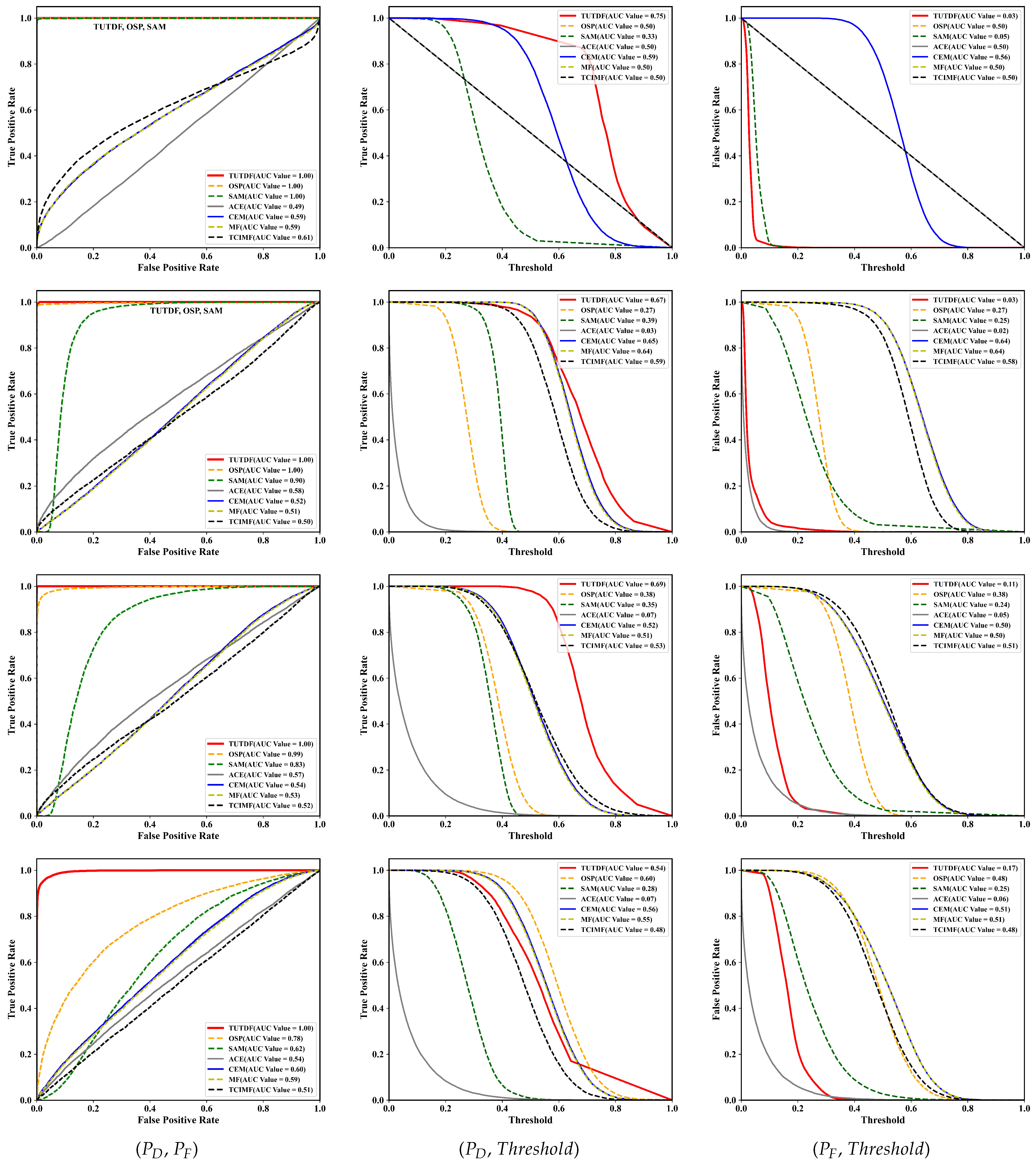
(1) Evaluation Criteria: The traditional receiver operating characteristic (ROC) curve depicts the correlation between the false alarm rate (FAR) $P_F$ and target detection probability $P_D$, which can be formulated as Equations (21) and (22). The $P_F$ represents the portion of falsely detected pixels for the entire image:

$$P_F=\frac{N_F}{N}$$

(21)

where $N_F$ stands for the number of falsely detected pixels and N refers to the total number of pixels in the image. The target detection probability $P_D$ denotes the ratio between correctly detected pixels and target pixels among the whole image:

$$P_D=\frac{N_C}{N_T}$$

(22)

where $N_C$ is the amount of correctly detected pixels and $N_T$ refers to the number of target pixels in the entire image. Once the detection result maps are given, we can set a series threshold $\tau$ to obtain many ($P_D$,$P_F$) to generate the ROC curve. The closer the ROC curve of ($P_D$,$P_F$) is to the upper left corner, the better the detection effect. Meanwhile, the area under the curve (AUC) of ($P_D$,$P_F$) is used for quantitative evaluation. The larger the AUC value, the better the detection effect.

However, a traditional ROC curve of ($P_D$, $P_F$) can only be used to evaluate the effectiveness of a detector, not target detectability (TD) or background suppressibility (BS). For a more comprehensive evaluation, we adopted a new 3D ROC curve [24,25]. Compared with the traditional ROC curve, the 3D ROC curve criterion, in the form of its three derived 2D ROC curves of ($P_D$, $P_F$), ($P_D$,$\tau$ ), and ($P_F$,$\tau$ ) can further be used to evaluate the effectiveness of a detector and its TD and BS, which can be quantified as:

$$0\le AU{C}_{TD}=AU{C}_{(D,F)}+AU{C}_{(D,\tau )}\le 2$$

(23)

$$-1\le AU{C}_{BS}=AU{C}_{(D,F)}-AU{C}_{(F,\tau )}\le 2$$

(24)

where $AU{C}_{(D,F)}$, $AU{C}_{(D,\tau )}$ and $AU{C}_{(F,\tau )}$ represent the AUC value of the ROC curve of ($P_D$, $P_F$), ($P_D$, $\tau$) and ($P_F$, $\tau$), respectively. The calculated $AU{C}_{TD}$ and $AU{C}_{BS}$ are employed to quantitatively characterize the detector’s TD and BS, respectively.

(2) Experimental Settings: We used the spectral imager with SpecView software to calibrate the reflectance of the raw images and utilized ENVI 5.3 to perform HSI cropping and waveband selection. Subsequent experiments were based on an Intel(R) Core(TM) i9-12900KF CPU, GeForce RTX 3080 Ti GPU, 64 GB RAM, Windows 11 OS, and the code was based on Python 3.9 and the deep learning framework PyTorch 1.12.1. The relevant parameters of the experimental dataset are shown in

Table 1. Target detection network training dataset parameters.

Material	Target Pixels	Water Pixels	Number of Depth	Synthetic Data	Water Data	Source Domain
Iron	10	10	100	10,000	10,000	6
Stone	10	10	100	10,000	10,000	6
Rubber	10	10	100	10,000	10,000	5

,

Table 2. Depth estimation network training dataset parameters.

Material	Target Pixel	Water Pixel	Depth Range	Number of Depth
Iron	10	10	0–2.5 m	250
Stone	10	10	0–2.0 m	200
Rubber	10	10	0–1.0 m	100

and

Table 3. Test dataset parameters.

Material	Size	Depth
Iron	100 × 100	0.1 m, 0.5 m, 1.0 m, 1.6 m
Stone	100 × 100	0.4 m, 0.7 m, 1.6 m, 1.9 m
Rubber	100 × 100	0.1 m, 0.3 m, 0.6 m, 0.9 m

.

3. Results

To demonstrate the superiority of our proposed method, we compared TUTDF with traditional land-based hyperspectral target detection methods—MF [26], CEM, ACE [27], OSP, SAM [28], and TCIMF [29]—using different materials and depths. The ground truth of the datasets in Figure 16, Figures 18 and 19 are manual tagging according to pseudo-color images.

3.1. Iron Plate

First and foremost, we will demonstrate the detection performance from a visual standpoint by Figure 16. Depending on the visual judgment, the TUTDF possessed the slightest visible difference from the ground truth. Furthermore, as compared to other detectors, TUTDF was able to reduce the negative influence of background pixels by detecting the fewest background pixels. However, traditional land-based target detection algorithms fared poorly across all datasets because the target and background were no longer independent in underwater contexts.

To conduct a qualitative analysis of the detection results, the ROC curves of ($P_D$, $P_F$), ($P_D$, $\tau$) and ($P_F$, $\tau$) were plotted in Figure 17 as a further three critical comparison metrics. The ROC curves of ($P_D$, $P_F$) of our method remain over other curves in all depths. Among the other detectors, OSP and SAM perform well when the target is shallower, but when the target is deeper, their performance decreases. The ACE detector fails at all depths. For the ROC curves of ($P_D$, $\tau$), ACE occurred at the lower right, which demonstrated its invalid TD. TUTDF was located upwards from the other methods used for comparison at each depth, except 1.6 m, where it was placed slightly lower than some other methods. Moreover, the ROC curves of ($P_F$, $\tau$) of the TUTDF were located at the bottoms of other methods used for comparison at each depth, except ACE. However, ACE is invalid. Based on these three curves, we could conclude that TUTDF has a better detection performance compared with the lower FARs, even when the target is deeper, and other methods have failed.

For a quantitative comparison, as shown in

Table 4. AUC values calculated from the three 2D ROC curves of different detection results on iron at various depths.

Depth	Detector	AUC($\mathit{D},\mathit{F}$)	AUC($\mathit{D},\mathit{\tau }$)	AUC($\mathit{F},\mathit{\tau }$)	AUC${}_{\mathit{TD}}$	AUC${}_{\mathit{BS}}$
0.1 m	TUTDF	1.00	0.75	0.03	1.75	0.97
	OSP	1.00	0.50	0.50	1.50	0.50
	SAM	1.00	0.05	0.05	1.05	0.95
	ACE	0.49	0.50	0.5	0.99	−0.01
	CEM	0.59	0.59	0.56	1.18	0.03
	MF	0.59	0.50	0.50	1.09	0.09
	TCIMF	0.61	0.50	0.50	1.11	0.11
0.5 m	TUTDF	1.00	0.67	0.03	1.67	0.97
	OSP	1.00	0.27	0.27	1.27	0.73
	SAM	0.90	0.39	0.25	1.29	0.65
	ACE	0.58	0.03	0.02	0.61	0.56
	CEM	0.52	0.65	0.64	1.17	−0.12
	MF	0.59	0.64	0.64	1.23	−0.05
	TCIMF	0.50	0.59	0.58	1.09	−0.08
1.0 m	TUTDF	1.00	0.69	0.11	1.69	0.89
	OSP	0.99	0.38	0.38	1.37	0.61
	SAM	0.83	0.35	0.24	1.18	0.59
	ACE	0.57	0.07	0.05	0.64	0.52
	CEM	0.54	0.52	0.50	1.06	0.04
	MF	0.51	0.51	0.50	1.02	0.01
	TCIMF	0.52	0.53	0.51	1.05	0.01
1.6 m	TUTDF	1.00	0.54	0.17	1.54	0.83
	OSP	0.78	0.60	0.48	1.38	0.30
	SAM	0.62	0.28	0.25	0.90	0.37
	ACE	0.54	0.07	0.06	0.61	0.48
	CEM	0.60	0.56	0.51	1.16	0.09
	MF	0.59	0.55	0.51	1.14	0.08
	TCIMF	0.51	0.48	0.48	0.99	0.03

The bold entries represent the best performance in each column at a certain depth.

, the AUC values of ($P_D$, $P_F$), ($P_D$, $\tau$), ($P_F$, $\tau$), TD and BS were also calculated. The AUC(D,F) values of TUTDF were higher than other detectors and remained at 1.00, while other detectors’ decreased with depth. Although the AUC ($P_D$, $\tau$) value of our proposed method at 1.6 m is slightly lower than OSP, when it comes to a more accurate TD-evaluating indicator AUC ${}_{TD}$, TUTDF is at least 0.16 higher than other detectors, proving its excellent target detection abilities. Furthermore, TUTDF attains the lowest FAR among all valid detectors, and the corresponding AUC ($P_F$, $\tau$) values were under 0.17 at all depths. Moreover, in terms of BS, TUTDF is also better than other detectors. When the target is at a deeper position, the AUC${}_{BS}$ values of TUTDF were much higher than other detectors, which can effectively suppress the interference of the water background.

3.2. Stone Disc

As shown in Figure 18 and

Table 5. AUC values calculated from the three 2D ROC curves of different detection results on STONE at various depths.

Depth	Detector	AUC($\mathit{D},\mathit{F}$)	AUC($\mathit{D},\mathit{\tau }$)	AUC($\mathit{F},\mathit{\tau }$)	AUC${}_{\mathit{TD}}$	AUC${}_{\mathit{BS}}$
0.4 m	TUTDF	1.00	0.75	0.03	1.75	0.97
	OSP	1.00	0.50	0.50	1.50	0.50
	SAM	1.00	0.05	0.05	1.05	0.95
	ACE	0.53	0.50	0.50	1.03	0.03
	CEM	0.51	0.59	0.56	1.10	−0.05
	MF	0.51	0.50	0.50	1.01	0.01
	TCIMF	0.44	0.50	0.50	0.94	−0.06
0.7 m	TUTDF	1.00	0.67	0.03	1.67	0.97
	OSP	1	0.27	0.27	1.27	0.73
	SAM	1.00	0.39	0.25	1.39	0.75
	ACE	0.53	0.03	0.02	0.56	0.51
	CEM	0.43	0.65	0.64	1.08	−0.21
	MF	0.47	0.64	0.64	1.11	−0.17
	TCIMF	0.43	0.59	0.58	1.02	−0.15
1.6 m	TUTDF	0.98	0.69	0.11	1.67	0.87
	OSP	0.91	0.38	0.38	1.29	0.53
	SAM	0.85	0.35	0.24	1.20	0.61
	ACE	0.51	0.07	0.05	0.58	0.46
	CEM	0.50	0.52	0.5	1.02	0.00
	MF	0.49	0.51	0.50	1.00	−0.01
	TCIMF	0.38	0.53	0.51	0.91	−0.13
1.9 m	TUTDF	0.81	0.54	0.17	1.35	0.64
	OSP	0.77	0.60	0.48	1.37	0.29
	SAM	0.73	0.28	0.25	1.01	0.48
	ACE	0.47	0.07	0.06	0.54	0.41
	CEM	0.49	0.56	0.51	1.05	−0.02
	MF	0.49	0.55	0.51	1.04	−0.02
	TCIMF	0.32	0.48	0.48	0.8	−0.16

The bold entries represent the best performance in each column at a certain depth.

, the test performance is consistent with iron when performed on the stone discs. From a material standpoint, the detection performance remains superior, even though the stone material has higher intraclass variability than the iron. Accordingly, we can conclude that the deep learning method trained using synthetic data can learn the underwater information of target pixels of the same material with differences and detect the target with low FAR.

3.3. Rubber Plate

The results of the rubber plate detection are shown in Figure 19 and

Table 6. AUC values calculated from the three 2D ROC curves of different detection results on RUBBER at various depths.

Depth	Detector	AUC($\mathit{D},\mathit{F}$)	AUC($\mathit{D},\mathit{\tau }$)	AUC($\mathit{F},\mathit{\tau }$)	AUC${}_{\mathit{TD}}$	AUC${}_{\mathit{BS}}$
0.1 m	TUTDF	0.99	0.75	0.03	1.75	0.97
	OSP	0.99	0.50	0.50	1.50	0.50
	SAM	0.99	0.05	0.05	1.05	0.95
	ACE	0.53	0.50	0.50	0.99	−0.01
	CEM	0.69	0.59	0.56	1.18	0.03
	MF	0.70	0.50	0.50	1.09	0.09
	TCIMF	0.73	0.50	0.50	1.11	0.11
0.3 m	TUTDF	0.98	0.67	0.03	1.67	0.97
	OSP	0.85	0.27	0.27	1.27	0.73
	SAM	0.71	0.39	0.25	1.29	0.65
	ACE	0.49	0.03	0.02	0.61	0.56
	CEM	0.62	0.65	0.64	1.17	−0.12
	MF	0.56	0.64	0.64	1.23	−0.05
	TCIMF	0.48	0.59	0.58	1.09	−0.08
0.6 m	TUTDF	0.89	0.69	0.11	1.69	0.89
	OSP	0.89	0.38	0.38	1.37	0.61
	SAM	0.74	0.35	0.24	1.18	0.59
	ACE	0.51	0.07	0.05	0.64	0.52
	CEM	0.60	0.52	0.50	1.06	0.04
	MF	0.53	0.51	0.50	1.02	0.01
	TCIMF	0.28	0.53	0.51	1.05	0.01
0.9 m	TUTDF	0.76	0.54	0.17	1.54	0.83
	OSP	0.74	0.60	0.48	1.38	0.30
	SAM	0.64	0.28	0.25	0.90	0.37
	ACE	0.51	0.07	0.06	0.61	0.48
	CEM	0.64	0.56	0.51	1.16	0.09
	MF	0.56	0.55	0.51	1.14	0.08
	TCIMF	0.28	0.48	0.48	0.99	0.03

The bold entries represent the best performance in each column at a certain depth.

. Due to the strong absorption properties of rubber material, the detection performance of the rubber plate is lower compared to iron and stone and can only be detected within a shallow depth range. However, our method still performed the best in terms of TD and BS. This further confirms the generalization ability of our proposed method, which can detect targets of different materials. The result also indicates that rubber, which is a typical submarine anechoic material used to avoid sonar detection, is also effective in avoiding hyperspectral detection in the visible band. Therefore, to more effectively detect underwater submarines, it is often necessary to use infrared bands or detect heat trails.

Due to the limits of the spectral imager’s shooting time and the processing of massive data volumes, achieving a real-time performance is difficult. We are primarily concerned with the time required to make a complete detection. All detection methods were conducted on CPU, and the final results were the average of the five run-times.

Table 7. Execution time of different methods.

Dataset	Execution Time (Second)
	TUTDF	MF	CEM	ACE	OSP	SAM	TCIMF
Iron	0.688	1.068	1.132	1.375	0.912	1.470	1.110
Stone	0.689	1.092	1.110	1.372	0.930	1.272	1.076
Rubber	0.687	1.072	1.210	1.374	0.890	1.428	1.100

The bold entries represent the best performance in each row.

shows that the execution time of TUTDF is much lower than the other methods used in our datasets (spatial size of 100 × 100, 120 bands). As seen in

Table 8. Execution time of different modules.

Dataset	Execution Time (Second)
	TUTDF	Spatial	Domain	Detection
Iron	0.688	0.039	0.348	0.301
Stone	0.689	0.040	0.345	0.304
Rubber	0.687	0.039	0.351	0.297

, the most time-consuming step is the domain prediction, subsequent parallel optimization with GPU acceleration may further reduce the TUTDF execution time, which is not discussed in detail here.

In sum, TUTDF can attain a superior detection performance in TD and BS and more in-depth detection. Additionally, it can quickly perform underwater target detection. Considering all aspects of the detection results, we are confident in concluding that the proposed detection framework, trained using synthetic data, is effective, reliable, and capable of achieving a remarkable detection performance in most underwater materials.

4. Discussion

This section discusses and analyzes the effectiveness of the domain adaptive method and the spatial–spectral process.

4.1. Effectiveness Evaluation of the Domain Adaptation

To evaluate the effectiveness of the domain adaptive method, we conducted a performance analysis of the domain adaptive method without the spatial–spectral process. Since the shallower targets all have higher $AU{C}_{(D,F)}$ values, we chose the deeper targets for comparison to reflect the differences more prominently, and conducted experiments on 1.6 m iron plates and 1.6 m stone discs, respectively. This process followed the proposed pipeline. The method without domain adaptation aims to sample 100 depths at equal intervals from 0 to $H_{deep}$; then, the network was trained and could detect the target directly.

The results under the conditions of a 1.6 m iron plate and stone disc are shown in Figure 20 and

Table 9. Comparison of effect with and without domain adaptive, ‘Yes’ is with domain adaptive, ‘No’ is without domain adaptive.

Test Data	${\mathbf{AUC}}_{(\mathit{D},\mathit{F})}$
	Yes	No
Iron (1.6 m)	1.00	0.88
Stone (0.5 m)	0.98	0.78

The bold entries represent the best performance in each row.

. Qualitatively, taking the domain adaptive method makes the detection results more clearly distinguishable; quantitatively, using the domain adaptive method makes the $AU{C}_{(D,F)}$ values significantly improve by 0.2.

Table 10. Interval settings of domains for different materials.

Iron	$D_1[0,0.4)$	$D_2[0.2,0.6)$	$D_3[0.4,0.8)$	$D_4[0.6,1.4)$	$D_5[1.2,2.0)$	$D_6[1.8,2.5]$
Stone	$D_1[0,0.4)$	$D_2[0.2,0.6)$	$D_3[0.4,0.8)$	$D_4[0.6,1.2)$	$D_5[0.9,1.7)$	$D_6[1.4,2.0]$
Rubber	$D_1[0,0.3)$	$D_2[0.2,0.5)$	$D_3[0.4,0.7)$	$D_4[0.6,0.9)$	$D_5[0.8,1.1)$

The unit of measurement is meter (m).

and

Table 11. Real and estimated depths of underwater targets of different materials. ‘R’ denotes ‘Real’, ‘E’ denotes ‘Estimated’.

Iron(R)	0.100	0.500	1.000	1.600
Iron(E)	0.051	0.445	0.978	1.551
Stone(R)	0.400	0.700	1.600	1.900
Stone(E)	0.350	0.623	1.577	1.875
Rubber(R)	0.100	0.300	0.600	0.900
Rubber(E)	0.121	0.317	0.610	0.903

The unit of measurement here is meter (m).

show the interval settings and depth estimation results. Suitable source domains can be selected without strictly accurate depth estimation results, and the corresponding domain-adaptive sub-networks can be used to perform the detection task more efficiently. Here, the parameter S in Equation (13) was set to 100.

4.2. Effectiveness Evaluation of the Spatial–Spectral Process

Unfortunately, noise-free HSI are not available on real data to evaluate the noise reduction performance. However, the effects of HSI before and after processing on the subsequent detection performance are considered as an indirect objective evaluation criterion. To discuss the influence of the spatial–spectral process on the detection performance, the table below compares the detection performance of submerged iron, stone, and rubber.

Intuitively, in

Table 12. The effect of the spatial–spectral process on the detection of iron plate: ‘Yes’ is with spatial–spectral process, ‘No’ is without spatial–spectral process.

Depth	0.1 m	0.5 m	1.0 m	1.6 m	Average
No
$AU{C}_{(D,F)}$	1.00	1.00	1.00	0.99	0.9975
Yes
$AU{C}_{(D,F)}$	1.00	1.00	1.00	1.00	1.00

The bold entries represent the best performance in each row.

,

Table 13. The effect of the spatial–spectral process on the detection of stone plate.

Depth	0.4 m	0.7 m	1.6 m	1.9 m	Average
No
$AU{C}_{(D,F)}$	1.00	1.00	0.78	0.77	0.8875
Yes
$AU{C}_{(D,F)}$	1.00	1.00	0.87	0.78	0.9125

The bold entries represent the best performance in each column.

and

Table 14. The effect of the spatial–spectral process on the detection of rubber plate.

Depth	0.1 m	0.3 m	0.6 m	0.9 m	Average
No
$AU{C}_{(D,F)}$	0.98	0.97	0.84	0.71	0.87
Yes
$AU{C}_{(D,F)}$	0.99	0.98	0.88	0.76	0.90

The bold entries represent the best performance in each column.

, since the spatial–spectral process contains an approximate mean filtering of the images, the detection results are less noisy and the target was more easily distinguishable from the background after the procedure was executed. After processing, the $AU{C}_{(D,F)}$ value of the detection results is qualitatively enhanced, particularly at greater depths.

The spatial–spectral process can enhance the efficiency of hyperspectral underwater target detection, especially when the target depth is relatively deeper and the distinction between the target and background is low. As seen in Table 8, this operation does not significantly increase detection time and is very effective for spatial information usage.

5. Conclusions

This paper used a deep learning method to detect underwater targets from HSI. For a low-altitude remote sensing scene, a framework named TUTDF is proposed. This particular framework consists of two large modules: the synthetic data module and the target detection module. Due to the difficulty of obtaining hyperspectral underwater target datasets, we proposed a transfer-based approach, which trained the synthetic data-based networks, then transferred them to real data scenarios. The proposed framework first developed an unsupervised network to obtain water-quality parameters, combined with the a priori information of the target that is to be detected and set different depth intervals to synthesize underwater target datasets for multiple source domains to train the networks. Then, we designed a domain prediction network to select the source domain that is closest to the target domain based on the depth information. Finally, we can transfer the trained networks to a real scenario to directly perform the detection task.

To verify the effectiveness of the method in real scenarios, we conducted extensive and quantitative indoor and outdoor experiments and then obtained hyperspectral underwater target datasets with accurate depth labels. The detection results for real data with different materials and depths show that the framework trained using synthetic data is valid and reliable, and the transfer from synthetic data domains to real-world domains is feasible. The proposed framework has a definite advantage in terms of TD, BS, and detection speed over traditional land-based detection methods.

In addition, we carried out some work in UAV underwater data acquisition; focusing on how to optimize the data acquisition and calibration methods to achieve real-time UAV underwater target detection will be the subject of future work.