Article

A Study on the Retrieval of Ozone Profiles Using FY-3D/HIRAS Infrared Hyperspectral Data

1
Key Laboratory of Infrared System Detection and Imaging Technologies, Shanghai Institute of Technical Physics, Chinese Academy of Sciences, Shanghai 200083, China
2
University of Chinese Academy of Sciences, Beijing 100049, China
3
Shanghai Institute of Technical Physics, Chinese Academy of Sciences, Shanghai 200083, China
4
Suzhou Academy, Shanghai Institute of Technical Physics, Chinese Academy of Sciences, Suzhou 215000, China
5
School of Atmospheric Sciences, Sun Yat-sen University, Zhuhai 519082, China
*
Author to whom correspondence should be addressed.
Remote Sens. 2023, 15(4), 1009; https://doi.org/10.3390/rs15041009
Submission received: 6 January 2023 / Revised: 9 February 2023 / Accepted: 10 February 2023 / Published: 12 February 2023
(This article belongs to the Special Issue Advances in Infrared Observation of Earth’s Atmosphere II)

Abstract

:
Atmospheric ozone is a pollutant gas that has an important influence on the process of atmospheric radiation transmission and climate change. The Fengyun-3D (FY-3D) satellite Hyperspectral Infrared Atmospheric Sounder (HIRAS) has better spectral performance than other remote sensing payloads. Its observation radiation data contains abundant atmospheric vertical information, which can be used for ozone retrieval, but there are no ozone profile business products being generated at present. Therefore, for the mainland of Hong Kong, based on HIRAS infrared hyperspectral observation data, we used the traditional one-dimensional variational (1D-VAR) physical retrieval algorithm, combined with the radiative transfer model for TOVS (RTTOV), and selected the spectrum channel according to the optimal sensitive profile algorithm. The artificial neural network (ANN) algorithm was used to optimize the prior profiles, and the atmospheric ozone profile retrieval system was established. Finally, a set of ozone profile retrieval schemes suitable for FY-3D/HIRAS were summarized. We used ERA5 reanalysis data and World Ozone and Ultraviolet Radiation Data Centre (WOUDC) data to determine true values. The retrieval results were compared with Global Forecast System (GFS) forecast data, Ozone Mapping and Profile Suite (OMPS) ozone products, and Atmospheric Infrared Sounder (AIRS) ozone products. The results show that our ozone profile retrieval scheme makes up for the shortcomings of the conventional physical methods in some atmospheric pressure levels. The overall root-mean-square error (RMSE) of the ozone from the ground to the top of the stratosphere is within 30% on average, which was better than that for the GFS forecast data; the retrieval accuracy RMSE (%) was less than 20% in the pressure layer with the highest ozone concentration (15–25 hPa), which is better than that of OMPS ozone products and AIRS ozone products. The retrieval results prove that FY3D/HIRAS observation data allow ozone profile retrieval. This paper provides a reference for generating independent HIRAS ozone profile product data sets in business, and provides support for the subsequent application of Fengyun-3 series meteorological satellites in atmospheric parameter remote sensing.

1. Introduction

Ozone is an important trace gas in the Earth’s atmosphere, and its concentration is unevenly distributed. Ozone affects the process of atmospheric motion in the stratosphere and troposphere and plays an important role in the process of atmospheric radiation transmission [1]. The ozone in the stratosphere accounts for 90% of the total ozone. Stratospheric ozone is a strong absorber of solar ultraviolet radiation and thus plays a role in protecting the Earth’s biosphere. In the troposphere, ozone is a greenhouse gas and a pollutant gas [2]. From 2009 to 2010, some scholars found that ozone pollution occurred frequently in China, especially in central and South China, and occurred especially in coastal cities [3,4,5]. Over the years, Guangdong, Hong Kong, and Macao have worked together to prevent and control air pollution in the region, forming an effective air quality management model in the Pearl River Delta [6]. The rapid economic development of the Guangdong–Hong Kong–Macao Greater Bay Area is facing an increasingly severe atmospheric ozone pollution problem, so ozone monitoring over the area is very important [7].
Satellite remote sensing has been widely used in atmospheric gas detection. Its main advantage is that it is not restricted by space, so it can obtain the spatial and temporal changes of atmospheric concentrations and other parameters in a large range. The channel weighting function of hyperspectral instruments is narrow, the observed brightness temperature changes are strong, and the hyperspectral instruments are highly sensitive to different gases at specific heights. With the gradual development of meteorological satellites, various countries have developed the infrared hyperspectral vertical probe payload on meteorological satellites. Business weather satellites with long-term operational planning and global coordination, which will be part of the future global hyperspectral atmospheric vertical exploration constellation system, will provide a global coverage of atmospheric temperature, humidity, cloud parameters, aerosols, greenhouse and trace gases, global radiation balance, and other integrated products. These high-spectral-resolution infrared atmospheric remote sensing instruments are equipped with a high precision on-orbit calibration system, which provides technical support for the accuracy and long-term stability of data [8]. The development of satellite infrared hyperspectral remote sensing makes up for the shortage of traditional methods of satellite vertical atmospheric detection, which are used in polar weather and climate research [9,10]. Among a large amount of satellite remote sensing data, infrared hyperspectral data, with their outstanding advantages of high spatial resolution and hyperspectral resolution, have become one of the largest contributing factors to the reduction of prediction errors and the improvement of assimilation effects [11]. High-resolution thermal infrared sensors can obtain a high-vertical-resolution of ozone distribution as well as night-time ozone distribution [12]. The FY-3D satellite was successfully launched on 15 November 2017 carrying the Infrared Hyperspectral Atmospheric Sounder (HIRAS) with 2275 spectral channels [13]. Developed by the Shanghai Institute of Technical Physics, Chinese Academy of Sciences, it is the first infrared hyperspectral detector in China’s polar-orbit meteorological satellites.
Atmospheric ozone detection is based on the absorbed and emitted radiation of the ozone. The most important physical property of the ozone is its absorption of spectral radiation, which is also the reason for studying the concentration of ozone in the atmosphere. Ozone has three obvious absorption bands for spectral radiation, namely the ultraviolet region near 220–330 nm, the yellow-green spectral region of visible light, and the infrared spectral region near 9.6 μm [14]. Referring to the absorption of ozone, the different physical quantities of atmospheric radiation after the actions of the atmosphere are measured near the absorption zone, and a corresponding radiative transfer model is established; according to the theory of atmospheric radiative transfer, the total amount or vertical distribution of ozone in the atmosphere can be retrieved by using proper algorithms [15]. Ma et al. [16] used Cross-Track Infrared Sounder (CrIS) for experimental data to obtain prior knowledge of ozone profiles by eigenvector statistics and carried out simultaneous iterative retrieval under the framework of the optimal estimation method; the maximum relative error was less than 20% in the stratosphere and the maximum relative error was less than 50% in the troposphere when the retrieval results were compared with the site data of WOUDC. Zhang et al. [17] used one-year temperature and ozone sounding data from Zhongshan Station, Amundsen–Scott (South Pole) Station, and Neumayer Station in 2008 to verify the accuracy of AIRS sixth-edition’s temperature and ozone vertical profile products in Antarctica. AIRS ozone retrieval accuracy in the stratosphere (RMSE: 25%) was better than that in the troposphere (RMSE: 30%), and the maximum value of RMSE appeared in the upper troposphere–lower stratosphere (UT–LS) region (up to 40%) and increased significantly in the ozone hole. Luo [18] carried out research on ozone profile retrieval and verification based on the detection characteristics and spectral data of Gaofen-5 (GF-5)/Atmospheric Infrared Ultra-Spectral Sounder (AIUS) and conducted cross-validation with Microwave Limb Sounder (MLS) ozone profile products. The relative deviation between the retrieval results and the MLS ozone profile was less than 10% from 20 to 50 km, indicating high retrieval accuracy. The relative deviation was greater than 20% at 10–15 km and 70–90 km. Pan [2] analyzed the distribution and variation characteristics of atmospheric ozone on a global scale using the total atmospheric ozone column retrieved from AIRS and Total Ozone Mapping Spectrometer (TOMS) satellite data. AIRS global’s (60°N–60°S) mean ozone column total values were approximately 3–5 Dobson units (DU) higher than the values of Total Operational Vertical Sounder (TOVS) and TOMS. Wang [19] studied the retrieval algorithm of the temperature–pressure and ozone profiles for AIUS and selected the suitable band in the infrared region for the occultation sensor. The improved statistical retrieval method based on eigenvectors was used to retrieve the temperature and pressure profiles, and the optimal estimation method was used to retrieve the ozone profiles. Above 60km, the retrieval result was different from that of the official product, similarly to a prior profile. Below 60km, the comparison accuracy with the official product was within ±20%. Cai [20] retrieved the atmospheric temperature and humidity profile of FY-4A/GIIRS (Geosynchronous Interferometric Infrared Sounder) based on an artificial neural network algorithm and verified it with the AIRS product. The average temperature RMSE in the troposphere was less than 1K, and the overall humidity below 200 hPa was better than 10%. Zhang et al. [21] retrieved temperature profiles from FY-3D/HIRAS data at different atmospheric pressure layers by a combination of neural networks and an improved one-dimensional variational algorithm. The RMSE values of temperature and humidity were improved by up to 0.5 K and 5%, respectively, based on the University of Wyoming’s sounding data. Comparing the temperature and humidity results with the GFS forecast field, the temperature’s RMSE was less than 1.5 K on average, which was better than that of the forecast data, and the humidity’s RMSE was less than 15%. Huang [22] retrieved the temperature profile of FY-4A/GIIRS data at different atmospheric pressure layers by combining the artificial neural network algorithm with an improved one-dimensional variational algorithm and evaluated the retrieval accuracy with the public sounding data of the University of Wyoming for the true value. The results showed that the average temperature error was less than 2K, and the retrieval accuracy was better than that of the temperature product published by GIIRS.
Based on the above analysis, at present, the similar infrared hyperspectral AIRS instrument, CrIS, and other instruments abroad have relatively mature ozone retrieval products, and the spectral band of domestic infrared hyperspectral instrument HIRAS also contains rich atmospheric information on absorption bands and has very mature temperature and humidity profile retrieval products but no mature ozone products. This is because the traditional one-dimensional variational retrieval algorithm used by mature temperature and humidity profile products in HIRAS is not suitable for ozone retrieval, so we used the traditional one-dimensional variational retrieval algorithm to retrieve the ozone profile and found that the retrieval accuracy was low under certain pressure levels. In this paper, the neural network method is added to the traditional retrieval algorithm for ozone retrieval in HIRAS for optimization, and an ozone profile retrieval scheme suitable for FY-3D/HIRAS is summarized. This retrieval scheme solves the above problems. The results show that FY-3D/HIRAS allows ozone retrieval and that high retrieval accuracy is obtained. FY-3D/HIRAS radiation data from Hong Kong in 2021 are selected in the experiment. The initial ozone profile is obtained through neural network and forecast data by matching the corresponding control data in time and space, and then the ozone profile is retrieved by the established retrieval system. Finally, the retrieval accuracy is compared and analyzed.

2. Instruments and Data

2.1. Instrument Introduction

FY-3D/HIRAS is the first infrared hyperspectral detection instrument of China’s polar-orbit meteorological satellite, with 2275 spectral channels providing infrared radiation spectra in three spectral bands: long-wave infrared (LWIR), 650–1135 cm−1; medium-wave infrared (MWIR), 1210–1750 cm−1; shortwave infrared (SWIR), 2155–2550 cm−1 [23]. The instrument’s design adopts the parallel observation of multiple small–plane arrays, which can prolong the formation time of an interferogram and form the instantaneous field of view of earth observation as much as possible. Three small arrays simultaneously observe the same field of view of the target on the ground, and four different target areas are simultaneously observed by the small array detectors in each wave band. Each detector has an earth observation angle of 1.1°, the instantaneous field of view of the corresponding substellar point is about 16 km, and the ground distance between pixels is 26.17 km [12]. Specific performance parameters are shown in Table 1.

2.2. Experiment Area and Time

The selected times and region of FY3D/HIRAS in 2021 were 05:00–06:00UTC on 13 January, 05:00–06:00 UTC on 24 February, 05:00–06:00 UTC on 26 May, 05:00–06:00 UTC on 28 July, 05:00–06:00 UTC on 18 August, 05:00–06:00 UTC on 10 November, and 06:00–07:00 UTC on 14 November in the transit area in Hong Kong. The selection of experimental data covered different months in spring, summer, autumn, and winter over the course of a year, and the specific dates and times were selected according to the data of the WOUDC station.

2.3. GFS Forecast Data

In this study, the GFS forecast data were input into the retrieval system to create an initial profile during retrieval. The GFS forecast data selected in this experiment were provided by the National Center for Environmental Prediction (NCEP) (https://www.ncdc.noaa.gov/data-access/model-data/model-datasets/global-forcast-system-gfs, accessed on 11 February 2023); the forecast time limit was 6 h, and the spatial resolution was 0.5°. We selected the GFS dataset collected with observations from FY-3D/HIRAS at the same time and in the same space. The dates were 18:00–00:00 UTC on 12 January, 18:00–00:00 UTC on 23 February, 18:00–00:00 UTC on 25 May, 18:00–00:00 UTC on 27 July, 18:00–00:00 UTC on 17 August, 18:00–00:00 UTC on 09 November, and 00:00–06:00 UTC on 14 November.

2.4. ERA5 Reanalysis Data

The ERA5 reanalysis data were used as the input information for RTTOV to obtain the simulated brightness temperature truth value, which was made up mainly of the ERA5’s daily average data set (https://apps.ecmwf.int/datasets/, accessed on 11 February 2023). The dates were 05:00–06:00 UTC on 13 January, 05:00–06:00 UTC on 24 February, 05:00–06:00 UTC on 26 May, 05:00–06:00 UTC on 28 July, 05:00–06:00 UTC on 18 August, 05:00–06:00 UTC on 10 November, and 06:00–07:00 UTC on 14 November. There are specific humidity profiles, temperature profiles, ozone profiles, a 2-m temperature, 2-m humidity, surface temperature, a 10-m wind U vector, a 10-m wind V vector, surface pressure, and pressure level information.

2.5. AIRS Data

The Version 7 (V7) L2 products from the AIRS suite of instruments are retrieved from Level 1B radiances, and include geophysical variables for temperature, water vapor, clouds and trace gases. AIRS L2 products from 13 January, 24 February, 26 May, 28 July, 18 August, 10 November and 14 November 2021 were selected (https://earthdata.nasa.gov/earth-observation-data/near-real-time/download-nrt-data/airs-nrt, accessed on 11 February 2023). Data from the same transit experimental area as HIRAS with a time difference of ±1 h were used.

2.6. WOUDC Site Data

The data from the Hong Kong site on 13 January, 24 February, 26 May, 28 July, 18 August, and 10 November 2021 were selected (https://woudc.org/data/explore.php?lang=en#, accessed on 11 February 2023). This is a vertical ozone profile of the atmosphere detected using the ozone-sonde Ecc. The WOUDC data archive can be searched by data category: there are six ozone data categories and three ultraviolet (UV) radiation data categories. The ozone dataset for the total ozone column includes total ozone and total ozone observations, and the vertical ozone profile includes LiDAR, ozonesonde, Umkehr N-value, and C-Umkehr. UV datasets for UV irradiance include broadband, multiband, and spectral.

2.7. OMPS Data

OMPS ozone products were selected on 13 January, 24 February, 26 May, 28 July, 18 August, 10 November, and 14 November 2021 (https://search.earthdata.nasa.gov/search/granules?q=omps, accessed on 11 February 2023). The Ozone Mapping and Profiling Suite (OMPS) was designed to measure the global distribution of total column ozone on a daily basis as well as the vertical distribution of ozone in the stratosphere and lower mesosphere (~15–60 km) using data from the same transiting experimental area and nearly at the same time as HIRAS.

3. Ozone Retrieval Experimental Process

3.1. Data Pre-Processing

In this experiment, FY-3D/HIRAS L1 observation data were downloaded, the data from 2021 were selected for retrieval, and the selected region was Hong Kong. Before forward retrieval, a Planck function was used to convert the HIRAS radiation value into a brightness temperature value. The Planck function is [25,26]:
M λ = 2 π h c 2 λ 5 [ e x p ( h c λ k T ) 1 ] 1
where, M λ is the radiant exitance, T is the temperature, λ is the wavelength, h is for the Planck constant, k is Ludwig Boltzmann’s constant, and c is the speed of light.

3.1.1. Spectral Data Apodization

FY-3D/HIRAS Ll data are unapodized. Spectral data need to be apodized in order to be followed up with a higher accuracy and to reduce side-lobe effects. The current HIRAS apodizing function is a Hamming function [23]. The light spectrum before and after apodization is shown in Figure 1.
In Figure 1, apod stands for apodized and unapod stands for unapodized. As one can see, the black line is unapodized and the red line is apodized. It can be seen that the burr phenomenon is reduced when the HIRAS spectrum undergoes apodization, and that the spectrum is smoother.

3.1.2. Selection of Clear Sky Pixels

Since the simulation accuracy of the radiation transmission mode is not high in the case of clouds, the judgment conditions for our clear sky samples were as follows: in the experiment, we selected the observation data of five representative infrared channels (810, 830, 850, 870, and 890 cm−1) in the long-wave window region, whose brightness temperature was greater than 290 K, and where the deviation of the observed brightness temperature from the simulated brightness temperature of the window channel should have been less than 5 K [27].

3.2. RTTOV Model

RTTOV and the rapid radiative transmission mode are developed from the TIROS Operational Vertical Sounder (TOVS) Rapid radiative transmission mode developed by the European Centre for Medium Range Weather Forecasts (ECMWF) in the early 1990s [28]. RTTOV can quickly and accurately simulate all kinds of satellite instruments in given atmospheric state parameters under the observed brightness temperature and can also quickly calculate the observed radiation on the atmospheric state (each layer’s temperature and absorption of gas) for the Jacobian matrix [29].

3.3. Observation Error Correction

The traditional one-dimensional variational physical retrieval algorithm and the variational assimilation theory assume that the observation field is unbiased, but due to the radiative transfer model error and the satellite observation error, in actual observation field retrieval, a system error often exists. The observations used in the retrieval of the deviation correction were needed before the experiment [30]. The mean of the observation error in the conventional 1D-Var retrieval algorithm is shown in Equation (2) [31]:
E = ( Y F ( x ) ) n ,
where E is the mean of the observation error, F(x) is the forward simulated brightness temperature, Y is the satellite observation, x is the atmospheric state parameter, and n is the number of samples.
The observation correction algorithm is used to calculate the average error, E, between the simulated brightness temperature and the observed brightness temperature. When the observation data are biased, the average error, E, needs to be subtracted from the observed brightness temperature to achieve the purpose of correcting the observed brightness temperature. The observation error covariance is also calculated based on the observed brightness temperature corrected by the average error, E. The correction of the observation error is shown in Equation (3) [26]:
S δ = ( Y F ( x ) E ) 2 n 1 ,
where S δ is the corrected observation error, E is the average error, F(x) is the forward simulated brightness temperature, Y is the satellite observation, x is the atmospheric state parameter, and n is the number of samples.

3.4. Observation and Background Errors

The RTTOV radiative transfer mode was used to calculate the forward modeling spectral brightness temperature data and Jacobian matrix. The FY-3D/HIRAS-observed spectral data, ERA5 reanalysis data, and GFS forecast data were interpolated in time and space. The time interpolation was based on the time of the observed data, and the reanalysis data of two adjacent times were selected for linear interpolation. For spatial interpolation, we used a cubic spline interpolation algorithm to perform spatial interpolation on the reanalysis data according to the geographic location information of satellite observation data. Then, we calculated the observation error covariance and background error covariance.

3.4.1. Observation Error Covariance Matrix

Observation errors are regarded as independent among channels, so the covariance matrix of observation errors is a diagonal matrix, whose diagonal elements are:
ε = ( Y m F ( x ) ) 2 n 1 .
In the equation above, Y m is the brightness temperature observed by FY-3D/HIRAS, m is the number of preferred channels participating in the retrieval, F(x) is the simulated brightness temperature calculated by the atmospheric state vector, X, from the reanalysis data from the RTTOV forward model, and n is the number of samples.

3.4.2. Background Error Covariance Matrix

The background error covariance describes the error (background field error) and correlation between the predicted value and the true value of the atmospheric state vector at each layer [32]. Two kinds of background error covariances were used in the experiment. One was obtained from the bias statistics of GFS forecast data and ERA5 reanalysis field data, and the other was obtained from the initial background profile obtained by integrating the neural network training data, the GFS forecast data, and the bias statistics of ERA5 reanalysis field data. The calculation formula of background error is as follows:
s i j = c o v ( x i , x j ) = 1 n k = 1 n [ ( x k i E ( x i ) ) ( x k j E ( x j ) ) ] ,
where x represents the background error—namely, the error between the background field and the real field; x k i is the kth sample data in the ith layer; E ( x i ) is the mean error of the ith layer forecast value; n is the total number of samples.

3.5. Channel Selection and ER (Entropy Reduction) and DFS (Degrees of Freedom for Signal) Calculation

3.5.1. Channel Selection

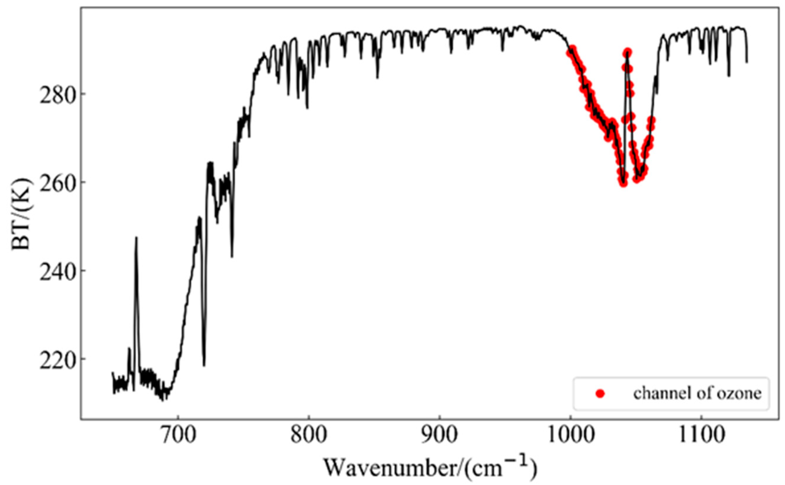
FY-3D/HIRAS infrared hyperspectral data show 2275 spectral channels (the spectral resolution of the three infrared bands is 0.625 cm−1). Using all channels for retrieval cannot improve the accuracy of the results because the feature information of some channels is similar and because there is a correlation between channels. Some channels are affected by multiple atmospheric parameters. Therefore, it is important to select the appropriate channel for atmospheric parameter retrieval. The general principle of channel selection is to select a channel that is only sensitive to the retrieval parameters [20]. The optimal sensitivity profile method (OSP) proposed by Crevoisier was used to select CO2 channels using AIRS data [33]. However, we improved the OSP algorithm. In the original algorithm, one-tenth of the signal-to-noise ratio (SNR) of the first channel in each barometric layer was taken as the threshold value, and the channels whose Jacobian peak value was at the same height but whose SNR was less than the threshold value were eliminated. We found in the experiment that there was little difference in the SNR between the adjacent channels, in fact, so the SNR of the first channel in each barometric layer was directly set as the threshold value, and channels whose Jacobian peak was at the same height but whose SNR was less than the threshold value were eliminated. In this way, more similar channels can be eliminated and information redundancy between channels can be avoided. Figure 2 shows that we selected 100 channels with a range of 1000–1061.875 cm−1. The selected ozone channels are as follows.
The concentration of the ozone channel near 1000 cm−1 and the peak of the weight function covering most of the barosphere provide the basis for the ozone retrieval below.

3.5.2. ER and DFS Calculation

The DFS indicates the useful independent signal in the measurement vector, where the higher the DFS, the more sufficient the target information contained in the observation. The ER can quantitatively describe the amount of information in the observation. The higher the DFS and ER, the more sufficient the target information contained in the observation, and the stronger the retrieval ability of the satellite. Generally, when the DFS of a certain parameter is greater than 0.5, the parameter can be obtained through observation retrieval [33].
The average kernel function, A, represents the sensitivity of the retrieval profile relative to the real profile. The calculation formula is as follows [34,35]:
A = ( K T S ε 1 K + S a p 1 ) 1 K T S ε 1 K ,
where K is the Jacobian matrix, representing the sensitivity of the observed values of each channel with respect to atmospheric parameters. x ^ is the quantity to be retrieved, x is the state vector, and Y is the satellite observation vector (radiation or brightness temperature). The DFS of the observation system for the A parameter is the sum of the diagonal elements of matrix A, namely the trace of matrix A. The ER contained in the observation process is [36]:
H = 1 2 l n | S a p | 1 2 l n | S ^ | ,
H = 1 2 l n | S a p · S ^ 1 | ,
where S a p is the background error covariance, S ^ is the post-observation error covariance matrix, and the absolute value sign in the above formula represents the determinant of the matrix.
Since the satellite remote sensing observation value is the emissivity value or brightness temperature value, which belongs to indirect observation and cannot be used to obtain S ^ by the direct use of observation information, it needs to combine the background field information. Therefore, the estimation of S ^ 1 can be written as:
S ^ 1 = K T S ε 1 K + S a p 1 ,
Substitute Formula (9) into Formula (8) to get:
H = 1 2 l n | S a p · ( K T S ε 1 K + S a p 1 ) | ,
The DFS and ER were calculated according to the above formula and are shown in Table 2.
As can be seen from the table, the DFSs are all above 0.5. The results show that the retrieval of ozone by HIRAS is feasible.

3.6. Neural Network Algorithm

On the basis of the traditional physical retrieval method, a new method for the joint retrieval of a neural network and the physical method were added in this experiment, that is, the neural network algorithm was used to optimize the initial field. In the model’s training, the first three to five days of the observation data of the monthly experimental data were used as the input data set of the training set. The model’s training input was the brightness temperature, which was the radiance-to-brightness temperature mentioned in Section 3.1. The corresponding time- and space-matched ERA5 reanalysis data were used as the output data set of the training set, while the training output was ozone profile data. After the training was completed, the network was saved for testing, and then the experimental data were input into the network model as test set data for testing, the results of which were saved. The test results and GFS data were compared with the ERA5 data, and the RMSE of each layer was obtained. The data with low RMSE values were selected and integrated to obtain a new initial profile, which was finally input into the retrieval system.
The schematic diagram of the neural network algorithm in this experiment is shown in Figure 3.
As shown in the schematic diagram, the neural network used in this experiment was set with a hidden layer. Input was the input layer and output was the output layer, both of which were connected to the hidden layer. Neurons in the adjacent layers between the two pairs were connected by the weight, W, intercept b, and activation function. In the experiment, the activation function was the sigmoid function.
Before training the training set, the data needed to be normalized; because the magnitude difference between different ozone concentrations in the atmosphere was large, the normalization formula is as follows [37]:
O 3 = 1 2 + 1 2 ( ( a c t a n ( O 3 A ) 0.01 ) / π 2 ) ,
A =   O 3 m a x   O 3 m i n 2 ,
where O3 is the ozone data of ERA5, and O3′ is the normalized ozone data of ERA5, both of which were then used as the output layer of the training set; O3max is the maximum ozone per layer and O3min is the maximum ozone per layer.

3.7. One-Dimensional Variational Retrieval Algorithm

Atmospheric parameter retrieval is based on the known satellite observation radial brightness temperature solving integral equations of radiative transfer. There is no single solution. How to solve the problem of the integral equation is the key to the atmospheric parameter remote sensing retrieval problem. The main retrieval methods are the statistical regression method, a neural network algorithm, and the physical retrieval method [38].
In this study, we used the physical retrieval method to retrieve the atmospheric ozone profile. The retrieval of the atmospheric ozone profile was mainly based on the basic theory of the atmospheric radiative transfer equation because the atmospheric ozone parameter based on FY-3D/HIRAS observation is a nonlinear problem, and because the iterative method is usually used to approach the true solution of the nonlinear problem. In the process of the retrieval of atmospheric composition by physical retrieval, the core aim was to construct the objective function and determine an iterative optimization method. In this study, two retrieval algorithms were used to retrieve the ozone profile. The first method was to use GFS forecast data as the initial field input into the one-dimensional variational retrieval system for retrieval to obtain an ozone profile. The first method is referred to as 1Dvar below. The second method was based on the neural network algorithm described above to optimize the initial field and obtain a new initial profile, which was input into the retrieval system to obtain an ozone profile. The second method will be called Ann_1Dvar.
The one-dimensional variational retrieval algorithm considers the process of atmospheric radiation transmission, combines the observation value, prior background value and error information, and transforms the nonlinear equation into an optimization problem. The retrieval process is used mainly for the purpose of constructing an objective function (cost function) and an optimization strategy. The objective function is based on the one-dimensional variational retrieval method, which needs to consider the atmospheric radiation transmission process, and in which retrieval is performed by combining the observation value, prior value, and error information [39].

3.7.1. Building the Objective Function

For the retrieval of atmospheric parameters, it is essential to solve the objective function, J(X), and minimize it. With the prior background profile, X b , as the starting value, J(X) is minimized by constantly adjusting the atmospheric state column vector X (namely the atmospheric state profile) [39,40,41],
J ( X ) = { [ Y m F ( X ) ] T × S ε 1 × [ Y m F ( X ) ] } + { [ X X b ] T × γ S a p 1 × [ X X b ] } ,
where X b is the GFS forecast data, S a p is the background error covariance, S ε is the observation error covariance, F(X) is the simulated observation, Y m is the FY-3D/HIRAS observation data, the optimal number of channels involved in the retrieval is m, and γ is the Lagrange smoothness factor.

3.7.2. The Solution—The Newton Iteration

The atmospheric ozone profile was obtained by using the Newton nonlinear iterative method to minimize the above objective function, J(X). The general form of Newton’s nonlinear iterative equation is as follows [42]:
x n + 1 = x n [ 2 J ( x n ) ] 1 J ( x n ) ,
where J ( X n ) and 2 J ( x n ) are the first and second derivatives, respectively, specifically expressed as:
J ( x n ) = K T S ε 1 [ Y m F ( x ) ] + S a p 1 ( x x b ) ,
2 J ( x n ) = S a p 1 + K T S ε 1 K d 2 K T d x S ε 1 [ Y m F ( x ) ] ,
where K is the Jacobian matrix calculated by the radiative transmission mode. In the retrieval of satellite data, HIRAS radiation value data, Y m , and forward simulation observation radiation, F(x), are close to each other in the actual calculation, and [ Y m F ( x ) ] gradually decreases. In order to reduce the calculation amount, the second-order partial derivative of the objective function is usually ignored, and the final iterative equation is [43]:
X n + 1 = X n + ( S a p 1 + K n T S ε 1 K ) 1 [ S a p 1 ( X b X n ) + K n T S ε 1 ( Y m F ( X n ) ) ] ,
where n is the number of iterations, with X n + 1 and X n as the profile results of n + 1 and the nth iteration, respectively. In general, when the objective function, J ( x n ) J ( x n + 1 ) , is less than a certain threshold, it is regarded as convergence.

3.8. Setting up the Experimental System

The retrieval process mainly consists of constructing the objective function and determining an optimization method. The objective function is based on the one-dimensional variational retrieval method, which needs to consider the atmospheric radiative transmission process. The atmospheric parameters are retrieved by combining the observation value, prior value, and error information [33]. Newton’s iteration method is used to minimize the objective function and find a set of atmospheric states that minimize the difference between the observed and forward results. In the retrieval system established in this experiment, firstly, data preprocessing was performed on FY-3D/HIRAS L1 observation data. The linear interpolation method and cubic interpolation method were used to interpolate the observed data with the ERA5 reanalysis data and the GFS forecast data in time and space. Then, we input the processed observation data into the RTTOV mode to obtain the simulated brightness temperature and Jacobian matrix, and used the optimal sensitivity profile method to select the channel. In this study, two retrieval algorithms were used to retrieve the ozone profile. The first method was to use the GFS forecast data as the initial field input into one-dimensional variational retrieval system for retrieval to obtain ozone profile. The second method was based on the neural network algorithm described above to optimize the initial field and obtain a new initial profile, which was input into the retrieval system to obtain the ozone profile. Because the initial profile was different, two different covariances of background errors needed to be calculated separately. Finally, the background error covariance corresponding to the two initial profiles and the observation error covariance were input into the one-dimensional variational retrieval system, respectively, and the ozone profile was calculated using Newton’s nonlinear iteration method.
Finally, the retrieval results and the corresponding prior profiles were compared with the ERA5 reanalysis data for the initial estimation analysis. Then, the WOUDC site data, OMPS ozone products, and AIRS ozone products were compared and verified, and the results were analyzed and discussed. The retrieval system was built as shown in Figure 4. The black line in the figure represents the GFS forecast data input into the one-dimensional variational retrieval system as the initial profile. The blue line represents the input of the initial profile optimized by the neural network algorithm into the retrieval system. The red line represents the ozone profile retrieval scheme suitable for FY-3D/HIRAS.
After proving the ability of FY-3D/HIRAS to retrieve atmospheric ozone, a retrieval algorithm was created. The neural network algorithm was used to train the observation data, integrate the GFS forecast data and training results, and obtain the ozone profile, which was closer to the ERA5 reanalysis data as a new prior background profile in the one-dimensional variable retrieval system. Then, the two sets of retrieval results were compared and analyzed. Finally, a set of ozone retrieval methods suitable for FY-3D/HIRAS in different altitude ranges were proposed based on the accuracy verification results.

3.9. Conversion Formula Unit Unity and Error Evaluation and Analysis Method

3.9.1. MMR and VMR Conversion Formulas

Because the data unit used in ERA5 reanalysis data and GFS forecast data is the Mass Mixing Radio (MMR) ratio, whose unit is kg/kg, the common unit of ozone is the Volume Mixing Radio (VMR) ratio, whose unit is ppmv or ppbv. The MMR and VMR conversion formula of ozone is as follows:
V M R = 28.9644 47.9982 × e 6 × M M R .
After the unit conversion, the unit can be unified with all kinds of data and products for comparison.

3.9.2. Number Density to Volume Mixing Ratio VMR

The unit of Suomi OMPS L2 ozone products is number density, the unit of which is cm−3, which needed to be converted to the volume mixing ratio to achieve unity as follows:
V M R = O 3 _ o m p s × T _ o m p s 7.244 e 12 × P ,
where O3_omps is the ozone data of OMPS, T_omps is the temperature data of OMPS, 7.244 × 10¹² is the constant coefficient, and P is the atmospheric pressure.

3.9.3. Error Evaluation and Analysis Method

In this study, the retrieval accuracy is was evaluated by calculating the mean deviation mean error (ME) and RMSE. The smaller the RMSE between the retrieved ozone profile and the true ozone profile, the higher the accuracy of the retrieval algorithm is considered [23]. The error calculation formulas are as follows:
  M E = i = 1 n ( x i x i ) n ,
R M S E = i = 1 n ( x i x i ) 2 n ,
R M S E ( % ) = R M S E x i ,
M E ( % ) = M E x i ,
where x i is the retrieval value; x i is the true value; x i is the average of the true values; n is the number of samples.

4. Experimental Results

4.1. Experimental Results

Ozone Concentration Profile Obtained from Retrieval

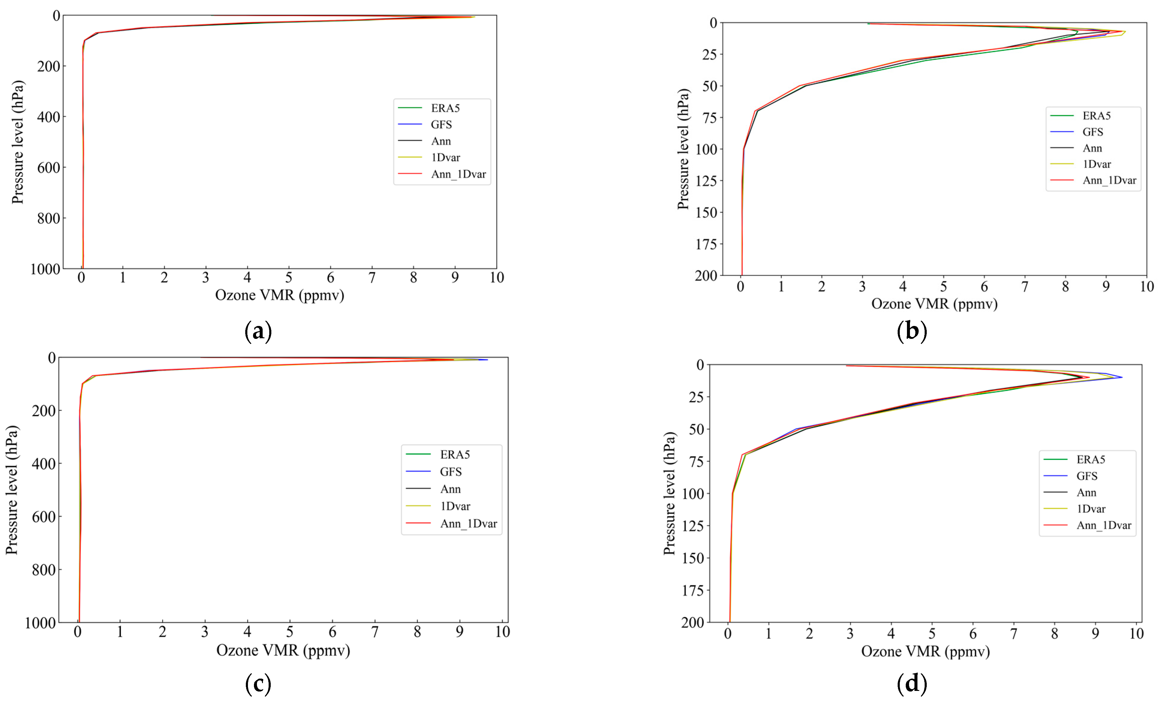
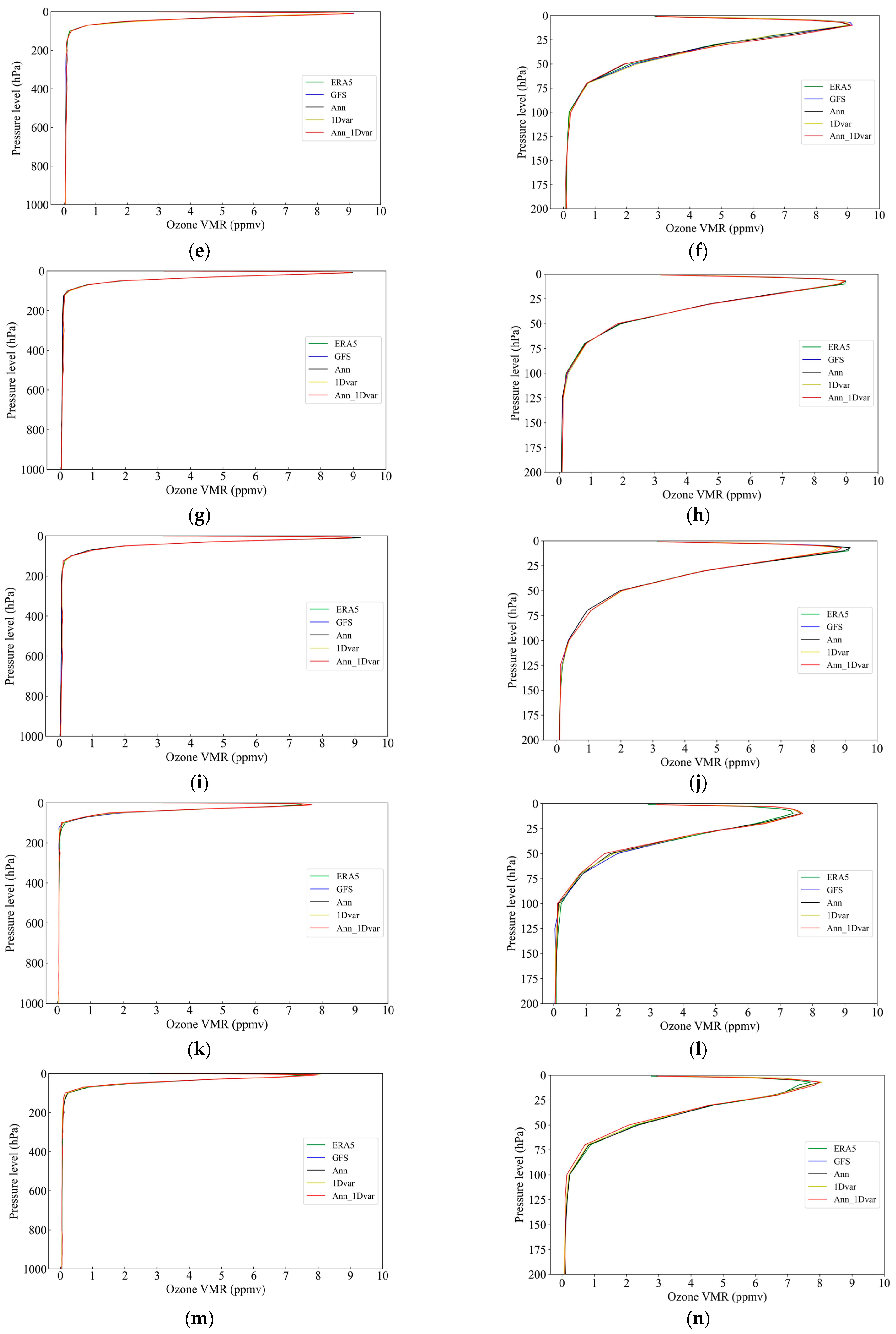
The retrieval results are shown in Figure 5. As shown in Figure 5, the retrieval results were consistent with the trend of the ozone concentrations across the data with respect to the altitude. The variation of the ozone concentration with altitude was as follows: the ozone concentration increased with the altitude and was most concentrated in the stratosphere. The peak was around 15–20 hPa.
From the retrieval results, it can be seen that the ozone concentration was high in spring and summer and low in autumn, rising in winter, and falling in summer. Ozone was concentrated in the upper stratosphere, and most of the ozone distribution was at 5–50 hPa; the maximum concentration was around 15–20 hPa, with a 125 hPa for the ground ozone concentration close to 0 ppmv.

4.2. Verification and Discussion of Experimental Results

4.2.1. Comparison and Discussion of Two Initial Profiles and Retrieval Results

With the two retrieval results and their corresponding initial profiles, the ERA5 reanalysis data were taken as the true value for initial analysis, and the WOUDC ozone site data were used as the true values for analysis and comparison. The comparison made was of the mean profiles of all the experimental data retrieved since 2021. The results with the ERA5 reanalysis data as the true value of the initial analysis are shown in Figure 6, and the results with WOUDC site data as the true value are shown in Figure 7.
As can be seen from Figure 6, both retrieval methods have higher accuracy than the GFS prediction data. At the highest levels of ozone concentration, the Ann_1Dvar method has the best accuracy. At 75–450 hPa, the precision of 1Dvar retrieval is the highest. At 450–800 hPa, the precision of Ann retrieval is the highest. At 800–1000 hPa, the precision of Ann 1Dvar retrieval is the highest.
The RMSE (%) of the two retrieval results and the ERA5 are all within 10% at the place with the largest concentration, and the ME (%) is very close to 0. The smaller the RMSE (%) is, the closer the ME (%) is to 0, indicating a higher retrieval accuracy. The results show that the Ann_1Dvar retrieval method is more accurate than the 1Dvar retrieval method at the 1–20-hPa position and in the place with the highest ozone concentration. In the stratosphere, the RMSE values (%) of 1Dvar retrieval methods are mostly within 30%, and the ME (%) is within ±10%. The RMSE values (%) of the two methods in 80–125 hPa were both large, but most of them are within 50%, and the RMSE (%) of the troposphere is within 40%. This implies that the 1Dvar retrieval method is more accurate than the Ann_1Dvar retrieval method in the middle, lower, and top troposphere. The RMSE (%) at 800–1000 hPa near the ground is within 30%, and the ME (%) is within ±15%. This implies that the Ann_1Dvar retrieval method has a higher accuracy than the 1Dvar retrieval method.
As can be seen in Figure 7, the RMSEs (%) of the two retrieval results and of the WOUDC site data are within 20% at 1–20 hPa, and ME (%) is within ±20%. The Ann_1Dvar retrieval method has higher accuracy than the 1Dvar retrieval method. At 25–100 hPa, the 1Dvar retrieval method has higher accuracy than the Ann_1Dvar retrieval method, but at 50–100 hPa, the RMSE (%) is larger, and the ME (%) is within ±40%. At 100–150 hPa, the RMSE (%) is within 60%, the ME (%) is within ±30%, and the Ann_1Dvar retrieval method is more accurate than the 1Dvar retrieval method. At 150–180 hPa, the RMSE (%) is within 50%, the ME (%) is within ±20%, and the 1Dvar retrieval method is more accurate than the Ann_1Dvar retrieval method.
It can be seen in Figure 6 and Figure 7 that, whether the true value is taken from ERA5 data or WOUDC site data, the Ann_1Dvar retrieval method has a higher accuracy than the 1Dvar method does at 1–25 hPa, and 1Dvar has a higher accuracy than Ann_1Dvar does at 25–100 hPa. The RMSE (%) at 50–125 hPa is relatively large, and, on the whole, the two retrieval methods are more accurate than the GFS forecast data and the new prior initial profile obtained by the integration of a neural network and GFS forecast data.

4.2.2. Comparison and Analysis of Retrieval Results with OMPS Data

OMPS (Ozone Mapping and Profiling Suite) was designed to measure the total global ozone column distribution and the vertical distribution of ozone in the stratosphere and lower mesosphere (15–60 km) on a daily basis. The OMPS on the Suomi NPP satellite consists of three instruments: nadir mapper (NM), nadir profiler (NP), limb profiler (LP), and OMPS, which are used for measurements in the middle and upper stratosphere using a UV wavelength and for those in the upper troposphere and lower stratosphere using a visible (VIS) wavelength. We used the Suomi OMPS L2 ozone product for comparison with the retrieval results. The ozone profile at 10–140 hPa retrieved from a visible wavelength was used in this experiment at the same time as the experimental data and FY-3D/HIRAS data were being selected to carry out atmospheric layer and spatial interpolation. We calculated the RMSE and ME by using the retrieval results and the OMPS product profile with the true values, and the calculation results are shown in the Figure 8 and Figure 9.
It can be seen in Figure 8 and Figure 9 that the accuracy of the two retrieval methods is higher than that of OMPS no matter whether the true value is taken from ERA5 data or WOUDC site data. In the place with the highest ozone concentration of 10–20 hPa, the Ann_1Dvar retrieval method is still more accurate than the 1Dvar method, but in other atmospheric pressure layers, the 1Dvar retrieval method retrieval accuracy is high.

4.2.3. Comparison and Analysis of AIRS Products and Retrieval Results

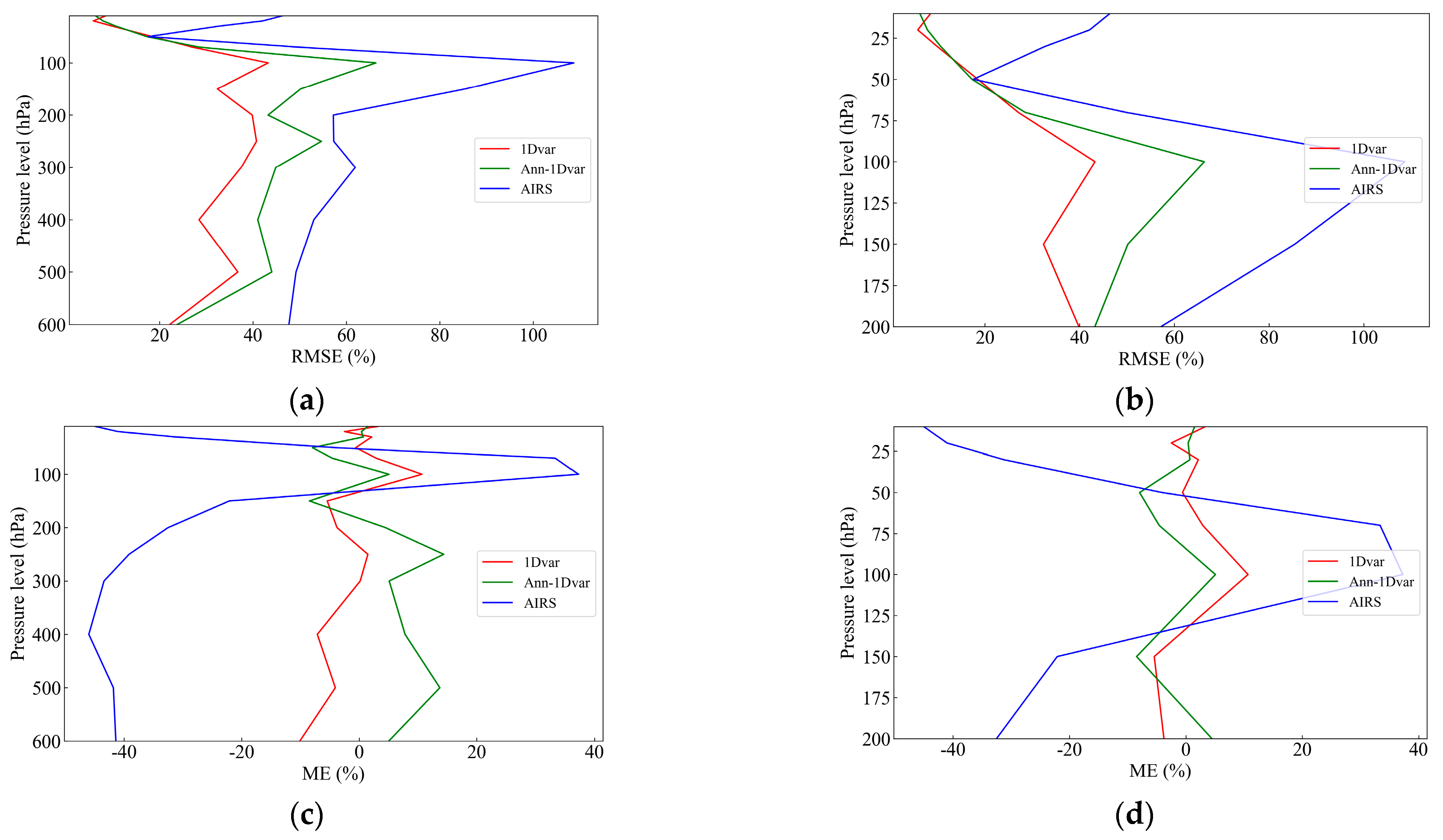
We also compared international instrument products and selected AIRS L2 products for comparative analysis because the ozone concentration does not change dramatically over time. For the experiment, we selected AIRS L2 products at the same time as HIRAS, mainly using the same area as HIRAS, with a time difference of ±3–4 h. Finally, figures from the ERA5 reanalysis data and WOUDC ozone site data were compared as the true values. We calculated the RMSE and ME by using the retrieval results and the AIRS product profile with the true values, and the calculation results are shown in the Figure 10 and Figure 11.
As can be seen in Figure 10, using a figure from the ERA5 data as the true value, the ozone retrieval results from FY-3D/HIRAS observations using a one-dimensional variational retrieval system are more accurate than those using AIRS ozone products. The ozone profile obtained by integrating the initial ozone profile with the neural network algorithm into the retrieval system is also more accurate than using the AIRS ozone product. Therefore, FY-3D/HIRAS has higher accuracy for ozone retrieval, and the data are relatively reliable.
Using a figure from the WOUDC site data as the true value, it can be seen from Figure 11 that the ozone retrieval results obtained from FY-3D/HIRAS observation data through the one-dimensional variational retrieval system and the initial ozone profile integrated by adding neural network algorithm input to the retrieval system are both more accurate than those of the AIRS ozone products on the whole. In the lower stratosphere and upper troposphere, AIRS ozone products have a higher accuracy. However, in the regions with the highest concentrations of ozone and from the troposphere to the near surface, the 1Dvar and Ann_1Dvar retrieval methods have a higher accuracy than AIRS ozone products do. Overall, the ozone retrieval results of FY-3D/HIRAS are more accurate than those of AIRS ozone products.

4.3. Effects of Temperature and Water Vapor on Ozone Retrieval

We explored the influence of temperature and humidity on ozone retrieval, and carried out a verification analysis with the ERA5 reanalysis data as the true value. The input values of temperature and humidity profiles used in the Ann_1Dvar and 1Dvar retrieval algorithms were from ERA5 reanalysis data. By changing the input value of the temperature and humidity profile and using the temperature and humidity profile data of the GFS forecast data, the corresponding retrieval results were changed. The ozone retrieval profile obtained after changing the input value of the temperature and humidity profile was 1Dvar2.0 and Ann_1Dvar2.0, as mentioned below. The error analysis is shown in Figure 12 below.
As shown in Figure 12, after the input value of the temperature and humidity profile is changed, the corresponding retrieval accuracy is changed. As can be seen from the figure, the specific situation is as follows: at 0–110 hPa, the 1Dvar retrieval algorithm has a lower RMSE (%) than the 1Dvar2.0 retrieval algorithm does, that is, 1Dvar retrieval has a higher accuracy and the 1Dvar2.0 retrieval algorithm is more accurate than the 1Dvar retrieval algorithm. In the whole atmosphere, the Ann_1Dvar2.0 retrieval algorithm has a higher accuracy than the Ann_1Dvar retrieval algorithm does. We will further explore the influence of temperature and humidity on ozone retrieval.

5. Discussion

The ozone retrieval method integrated in this experiment covers the whole height of the atmosphere and obtains a high-precision atmospheric ozone retrieval profile. We know from the experimental results that the concentration of ozone is changing, being higher in some months and lower in some months. In addition, ozone was mostly concentrated in the stratosphere, and the maximum concentration was near 10–25 hPa. Based on FY-3D/HIRAS data, Zhang et al. [21] retrieved the temperature and humidity profiles, and by comparing them, we obtained the ozone profiles. We proved the retrieval ability of FY-3D/HIRAS. We also proposed a set of ozone retrieval methods suitable for different altitude ranges, the results of which are in Table 3.
Ma [16] and Zhang [17] retrieved ozone profiles using CRIS data and AIRS data, whereas we successfully retrieved ozone profiles using FY-3D/HIRAS with a high accuracy. Figures from both the ERA5 reanalysis data and the WOUDC site data were used as true values, and the comparison between the retrieval results and the ozone products from AIRS and OMPS shows that the RMSE (%) of the retrieval results is better than 20% and that the ME (%) is within ±20% near the altitude layer with the highest ozone concentration. At the same time, we also used neural networks to optimize the initial profile. It can be seen that, after the addition of the neural network algorithm, especially in the stratosphere region where ozone is concentrated, the retrieval accuracy was significantly improved. It is necessary to use a neural network to optimize the initial profile, which has proven to be feasible. Although the retrieval accuracy has not been improved in some atmospheric layers, it is still of research significance. Further in-depth research will be carried out in the future to try to improve the entire atmospheric layer.
We also studied the influence of temperature and humidity on ozone retrieval. The preliminary analysis shows that the change of temperature and humidity has an impact on ozone retrieval, but subsequent research needs to continue to explore the influence of temperature and humidity on ozone retrieval. The retrieval method obtained in this experiment proves the ability of FY-3D/HIRAS to retrieve ozone profiles with good retrieval accuracy, but at the same time there is room for improvement. The experiment is of great significance. In later experiments, the number of samples can be increased, and the algorithm can be improved by comprehensively considering various factors affecting the experimental results so as to further improve the retrieval accuracy.
Finally, some problems should be further discussed. In some atmospheric layers, the accuracy of ozone retrieval was not improved, and the causes of these problems should be further studied. It can be seen from the experiments that temperature and humidity have an impact on ozone retrieval, and when the accuracy of the temperature and humidity profile input into the retrieval system decreases, the accuracy of the retrieval results are improved. More experiments are needed to verify this, and the influence of temperature and humidity on ozone retrieval will be explored in the future. In future experiments, the number of samples will be increased, the retrieval speed will be improved, the selection of channels will be more refined, and the influence of neural networks on other atmospheric layers and the influence of temperature and humidity on ozone retrieval will be explored, so as to further improve the retrieval accuracy. Meanwhile, retrieval also has many meaningful uses. Retrieval products are real-time profile products, and forecasters can combine numerical models to make short neighborhood forecasts. Retrieval results can be used to evaluate and analyze the requirements of instrument indicators and methods. The reliable retrieval of historical data can produce independent climate data sets.

6. Conclusions

In this paper, we used the FY-3D/HIRAS data on Hong Kong all year round to retrieve the atmospheric ozone profile and proposed a set of ozone retrieval methods suitable for different altitude ranges. The results show that FY-3D/HIRAS has the ability to retrieve ozone profiles and high retrieval accuracy is obtained. For the mainland of Hong Kong, based on HIRAS infrared hyperspectral observation data, we used the traditional one-dimensional variational (1D-VAR) physical retrieval algorithm combined with the RTTOV (radiative transfer for TOVS) radiative transfer model, and selected the spectrum channel according to the optimal sensitive profile algorithm. The artificial neural network (Ann) algorithm was used to optimize the prior profiles, and the atmospheric ozone profile retrieval system was established. Finally, a set of ozone profile retrieval schemes suitable for FY-3D/HIRAS was summarized. Figures from the ERA5 reanalysis data and the WOUDC site data were used as the true values in the experiment, and the comparison results with ERA5 show that the RMSE (%) of the area with the maximum ozone concentration was better than 10%. Most stratospheric RMSEs(%) were better than 30%, ME (%) was within ±10%, tropospheric RMSE (%) was larger, and near-surface RMSE (%) was better than 20%. Compared with the data of the WOUDC site, the RMSE (%) and ME (%) of the area with a maximum ozone concentration (20 hPa) were better than 20%. Comparing the ozone profiles retrieved by our retrieval scheme with the GFS forecast profiles, it was found that the ozone profiles retrieved by our retrieval scheme can meet the current retrieval accuracy requirements. The value obtained in our retrieval scheme is closer to the true value than the GFS data is, and most of the atmospheric pressure levels are better than those of the GFS, which proves that the retrieval results of our retrieval scheme have a high accuracy. In order to improve the stability and reliability of the retrieval system, a comparative analysis was conducted with the ozone products of AIRS L2 and OMPS L2. Under different pressure levels, the retrieval results of this system have a better accuracy. Preliminary results show that the product accuracy of this retrieval scheme can reach or exceed that of international instruments.
The experiment emphasizes that the retrieval system obtained by adding a neural network algorithm on the basis of the traditional one-dimensional physical retrieval algorithm is of high reliability and stability. Because our retrieval system does not rely on reanalysis for data that is difficult to obtain in real time, it can be applied to business operations and can be used as a reference for the production of related products. The multi-season long-time series ozone retrieval results show that the FY-3D/HIRAS spectral channel has a good ozone detection ability, which provides a basis for the generation of a HIRAS ozone product dataset, and also serves as support for subsequent research on ozone monitoring over the Guangdong–Hong Kong–Macao Greater Bay Area. In addition, with the successful launch of the infrared hyperspectral load FY-3E/HIRAS-II in the morning and evening orbit meteorological satellite, the observed samples were gradually enriched and improved, providing the possibility to further explore atmospheric gas retrieval based on the proposed method.

Author Contributions

Conceptualization, M.X., M.G. and P.H.; methodology, M.X., C.Z. and P.H.; software, M.X.; validation, M.X., P.H. and C.Z.; formal analysis, M.X. and M.G.; investigation, M.X., P.H. and T.Y.; resources, M.X.; data curation, M.X. and M.G.; writing—original draft preparation, M.X., M.G. and Y.H.; writing—review and editing, M.X., T.Y., P.H., C.Z. and C.Y.; visualization, M.G. and Y.H.; supervision, M.G. and Y.H.; project administration, M.G.; funding acquisition, M.G. All authors have read and agreed to the published version of the manuscript.

Funding

This research was funded by the Special Zones program for basic research of Shanghai (JCYJ-SHFY-2022-004).

Data Availability Statement

All the data generated or analyzed during this study are included in this article.

Acknowledgments

We would like to thank the NSMC (National Satellite Meteorological Center) for sharing FY3D/HIRAS data. We would also like to thank the ECMWF for their openly accessible data. Meanwhile, we also would like to thank Mingjian Gu and Yong Hu of the Shanghai Institute of Technical Physics, Chinese Academy of Sciences, for equipment and technical guidance.

Conflicts of Interest

The authors declare no conflict of interest.

References

  1. Wang, G.Q. Study of Atmosphere Ozone; Beijing Science Press: Beijing, China, 1985. [Google Scholar]
  2. Pan, L.; Niu, S.-J. A Comparison of Total Column Ozone Values Derived from AIRS, TOVS and TOMS. Remote Sens. 2008, 12, 54–63. [Google Scholar]
  3. Yao, Q.; Han, S.Q.; Cai, Z.Y.; Wang, J. The diurnal variation and ozone production potential of BTEX in Tianjin in the summer of 2012. China Environ. Sci. 2013, 33, 793–798. [Google Scholar]
  4. Yi, R.; Wang, Y.L.; Zhang, Y.J.; Shi, Y.; Li, M.S. Pollution characteristics and influence factors of ozone in Yangtze River Delta. Acta Sci. Circumstantiae 2015, 35, 2370–2377. [Google Scholar]
  5. Li, H.; Li, L.; Huang, C.; An, J.Y.; Yan, R.S.; Huang, H.Y.; Chen, M.H. Ozone source apportionment at urban area during a typical photochemical pollution episode in the summer of 2013 in the Yangtze River Delta. Environ. Sci. 2015, 36, 1–10. [Google Scholar]
  6. Zhong, L.J.; Louie, P.K.K.; Zheng, J.Y.; Yuan, Z.; Yue, D.; Ho, J.W.; Lau, A.K. Science-policy interplay: Air quality management in the Pearl River Delta region and Hong Kong. Atmos. Environ. 2013, 76, 3–10. [Google Scholar] [CrossRef]
  7. Zhan, S. Research on Changing Trend and Influencing Factors of Conventional Air Pollutants in Guangdong-Hong Kong-Macao Greater Bay Area; The University of Chinese Academy of Sciences (Guangzhou Institute of Geochemistry, Chinese Academy of Sciences): Beijing, China, 2018. [Google Scholar]
  8. Dong, C.-H.; Li, J.; Zhang, P. The Principle and Application of Satellite Hyperspectral Infrared Atmospheric Remote Sensing; Science Press: Beijing, China, 2013. (In Chinese) [Google Scholar]
  9. Boisvert, L.N.; Wu, D.L.; Vihma, T.; Susskind, J. Verification of air/surface humidity differences from AIRS and ERA-Interim in support of turbulent flux estimation in the Arctic. J. Geophys. Res. Atmos. 2015, 120, 945–963. [Google Scholar] [CrossRef]
  10. Boisvert, L.N.; Petty, A.A.; Stroeve, J.C. The impact of the extreme winter 2015/16 Arctic cyclone on the Barents-Kara Seas. Mon. Weather Rev. 2016, 144, 4279–4287. [Google Scholar] [CrossRef]
  11. Wang, Y.; Guan, L. Quality assessment of FY-4A’s geostationary interferometric infrared sounder observations data. Infrared Laser Eng. 2022, 51, 178–189. [Google Scholar]
  12. Keim, C.; Eremenko, M.; Orphal, J.; Dufour, G.; Flaud, J.-M.; Höpfner, M.; Boynard, A.; Clerbaux, C.; Payan, S.; Coheur, P.-F.; et al. Tropospheric ozone from IASI: Comparison of different inversion algorithms and validation with ozone sondes in the northern middle latitudes. Atmos. Chem. Phys. 2009, 9, 9329–9347. [Google Scholar] [CrossRef]
  13. Qi, C.-L.; Gu, M.-J.; Hu, X.-Q.; Wu, C. FY-3 Satellite infrared high spectral sounding technique and potential application. Adv. Met ST 2016, 6, 88–93. [Google Scholar]
  14. Pan, L. Ozone Profile Retrieval and Aerosol Classification Based on the Satellite Measurement; Nanjing University of Information Science and Technology: Nanjing, China, 2007. [Google Scholar]
  15. Liou, K.N. An Introduction to Atmospheric Radiation; China Meteorogical Press: Beijing, China, 2004. [Google Scholar]
  16. Ma, P.-F.; Chen, L.-F.; Zou, M.-M.; Zhang, Y.; Tao, M.-H.; Wang, Z.-F.; Su, L. Analysis of the Influence of Temperature on the Retrieval of Ozone Vertical Profiles Using the Thermal Infrared CrIS Sounder. Spectrosc. Spectr. Anal. 2015, 35, 3344–3349. [Google Scholar]
  17. Zhang, L.; Ding, M.H.; Bian, L.G.; Li, J. Validation of AIRS temperature and ozone profiles over Antarctica. Chin. J. Geophys. 2020, 63, 1318–1331. (In Chinese) [Google Scholar]
  18. Luo, Q. Ozone Profile Retrieval and Validation Research for Atmospheric Infrared Ultraspectral Spectrometer onboardGaoFen-5; University of Chinese Academy of Sciences: Beijing, China, 2020. [Google Scholar]
  19. Wang, Y. Research on Temperature/Pressure and Ozone Retrieval Algorithm Based on Atmospheric Infrared Ultraspectral Spectrometer; University of Chinese Academy of Sciences: Beijing, China, 2017. [Google Scholar]
  20. Cai, X.; Bao, Y.-S.; Petropoulos, G.P.; Lu, F.; Lu, Q.; Zhu, L.; Wu, Y. Temperature and Humidity Profile Retrieval from FY4-GIIRS Hyperspectral Data Using Artificial Neural Networks. Remote Sens. 2020, 12, 1872. [Google Scholar] [CrossRef]
  21. Zhang, C.; Gu, M.; Hu, Y.; Huang, P.; Yang, T.; Huang, S.; Shao, C. A Study on the Retrieval of Temperature and Humidity Profiles Based on FY-3D/HIRAS Infrared Hyperspectral Data. Remote Sens. 2021, 13, 2157. [Google Scholar] [CrossRef]
  22. Huang, P.-Y.; Guo, Q.; Han, C.-P.; Zhang, C.; Yang, T.; Huang, S. An Improved Method Combining ANN and 1D-Var for the Retrieval of Atmospheric Temperature Profiles from FY-4A/GIIRS Hyperspectral Data. Remote Sens. 2021, 13, 481. [Google Scholar] [CrossRef]
  23. Yang, T.-H. Tropospheric Wind Field Measurement Based on Infrared Hyperspectral Observations; University of Chinese Academy of Sciences: Beijing, China, 2020. [Google Scholar]
  24. Qi, C.L.; Zhou, F.; Wu, C.Q.; Hu, X.Q.; Gu, M.J. Spectral Calibration of Fengyun-3 high-spectral resolution infrared sounder. Opt. Precis. Eng. 2019, 27, 747–755. [Google Scholar]
  25. Zhao, Y. Principles and Methods of Remote Sensing Application Analysis; Science Press: Beijing, China, 2003. [Google Scholar]
  26. Ren, J. Study on the Atmospheric Temperature and Humidity Profiles of Satellite Remote Sensing Based on One-Dimensional Variational Algorithm. Master’s Thesis, Nanjing University of Information Science and Technology, Nanjing, China, 2018. [Google Scholar]
  27. Guan, Y.H.; Ren, J.; Bao, Y.S.; Lu, Q.; Liu, H.; Xiao, X. Research of the infrared high spectral (IASI) satellite remote sensing atmospheric temperature and humidity profiles based on the one-dimensional variational algorithm. Trans. Atmos. Sci. 2019, 42, 602–611. [Google Scholar]
  28. Saunders, R.; Matricardi, M.; Brunel, P. An improved fast radiative transfer model for assimilation of satellite radiance observations. Q. J. R. Meteorol. Soc. 1999, 125, 1407–1425. [Google Scholar] [CrossRef]
  29. Di, D.; Li, J.; Han, W.; Bai, W.; Wu, C.; Menzel, W.P. Enhancing the fast radiative transfer model for FengYun-4 GIIRS by using local training profiles. J. Geophys. Res. Atmos. 2018, 123, 12583–12596. [Google Scholar] [CrossRef]
  30. Bai, W.-G.; Zhang, P.; Zhang, W.-J.; Li, J. An efficient method for hyper-spectral infrared atmospheric radiation transfer calculation. J. Infrared Millim. Waves 2016, 35, 99–108. [Google Scholar]
  31. Zhu, L.H.; Bao, Y.S.; Petropoulos, G.P.; Zhang, P.; Lu, F.; Lu, Q.F.; Wu, Y.; Xu, D. Temperature and Humidity Profiles Retrieval in a Plain Area from Fengyun-3D/HIRAS Sensor Using a 1D-VAR Assimilation Scheme. J. Remote Sens. 2020, 12, 435. [Google Scholar] [CrossRef] [Green Version]
  32. Hewison, T.J. 1D-VAR retrieval of temperature and humidity profiles from a ground-based microwave radiometer. IEEE Trans. Geosci. Remote Sens. 2007, 45, 2163–2168. [Google Scholar] [CrossRef]
  33. Crevoisier, C. AIRS channel selection for CO2 and other trace-gas retrievals. Meteorol. Soc. 2003, 129, 2719–2740. [Google Scholar] [CrossRef]
  34. Menke, W. Geophysical Data Analysis: Discrete Inverse Theory; Academic Press: New York, NY, USA, 1984. [Google Scholar]
  35. Luo, S.; Di, D.; Cui, L.-L. Study on FY-4A/GIIRS infrared spectrum detection capability based on information content. J. Infrared Millim. Waves 2019, 38, 765–776. [Google Scholar]
  36. Rodgers, C.D. Information content and optimisation of high spectral resolution remote measurements. Adv. Space Res. 1996, 21, 136–147. [Google Scholar] [CrossRef]
  37. Pengyu, H.; Qiang, G.; Changpei, H.; Huangwei, T.; Chunming, Z.; Tianhang, Y.; Shuo, H. An Improved Method Combining CNN and 1D-Var for the Retrieval of Atmospheric Humidity Profiles from FY-4A/GIIRS Hyperspectral Data. Remote Sens. 2021, 13, 4737. [Google Scholar]
  38. Zhang, C.; Qi, C.; Yang, T.; Gu, M.; Zhang, P.; Lee, L.; Hu, X. Evaluation of FY-3E/HIRAS-II Radiometric Calibration Accuracy Based on OMB Analysis. Remote Sens. 2022, 14, 3222. [Google Scholar] [CrossRef]
  39. Boukabara, S.-A.; Garrett, K.; Chen, W.; Iturbide-Sanchez, F.; Grassotti, C.; Kongoli, C.; Chen, R.; Liu, Q.; Yan, B.; Weng, F.; et al. MiRS: An All-Weather 1DVAR Satellite Data Assimilation and Retrieval System. IEEE Trans. Geosci. Remote Sens. 2011, 49, 3249–3272. [Google Scholar] [CrossRef]
  40. Yang, J.; Min, Q. Retrieval of Atmospheric Profiles in the New York State Mesonet Using One-Dimensional Variational Algorithm. J. Geophys. Res. Atmos. 2018, 123, 7563–7575. [Google Scholar] [CrossRef]
  41. Jang, H.S.; Sohn, B.J.; Chun, H.W.; Li, J.; Weisz, E. Improved AIRS temperature and moisture soundings with local a priori information for the 1DVAR method. J. Atmos. Ocean. Technol. 2017, 34, 1083–1095. [Google Scholar] [CrossRef]
  42. Duncan, D.I.; Kummerow, C.D. A 1DVAR retrieval applied to GMI: Algorithm description, validation, and sensitivities. J. Geophys. Res. Atmos. 2016, 121, 7415–7429. [Google Scholar] [CrossRef]
  43. Martinet, P.; Dabas, A.; Donier, J.M.; Douffet, T.; Guillot, O.G.R. 1D-Var temperature retrievals from microwave radiometer and convective scale model. Tellus A Dyn. Meteorol. Oceanogr. 2015, 67, 27925. [Google Scholar] [CrossRef] [Green Version]
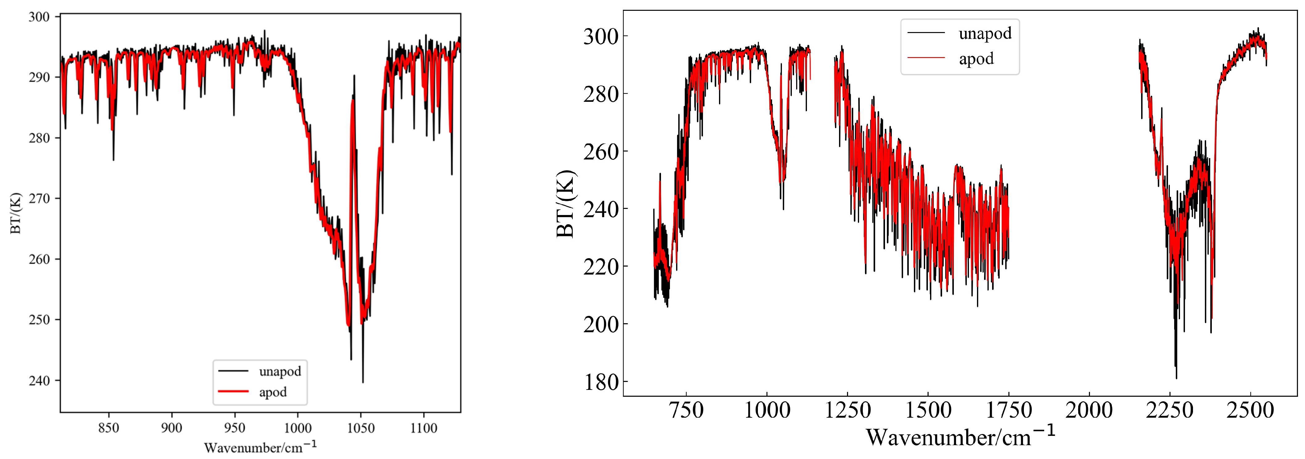
Figure 1. Comparison of light spectrum before and after apodization.
Remotesensing 15 01009 g001
Figure 2. The position of the ozone channel in the spectrum.
Remotesensing 15 01009 g002
Figure 3. Schematic diagram of neural network algorithm.
Remotesensing 15 01009 g003
Figure 4. Set-up of the retrieval system.
Remotesensing 15 01009 g004
Figure 5. The ozone concentration retrieval profile—(a,b) 2021_0113_0550, (c,d) 2021_0224_0555, (e,f) 2021_0526_0530, (g,h) 2021_0728_0535, (i,j) 2021_0818_0535, (k,l) 2021_1110_0540, and (m,n) 2021_1114_0605—and (o,p) the mean profile of retrieval results of all experimental data from 2021. The column on the left is the ozone concentration profile for 0–1000 hPa, and the column on the right is the ozone concentration profile for 0–200 hPa. The green line, ERA5, is the ERA5 ozone profile. The blue line, GFS, is the ozone profile of GFS forecast data. The black line, Ann, is the initial profile of neural network model and GFS data synthesis. The yellow line, 1Dvar (one-dimensional variational), is the traditional 1D-VAR physical retrieval algorithm retrieval ozone profile result obtained with GFS data as the initial profile, and the red line, Ann_1Dvar, is the retrieval result obtained by adding the neural network method to optimize the initial profile combined with the traditional 1D-VAR physical retrieval algorithm.
Remotesensing 15 01009 g005aRemotesensing 15 01009 g005bRemotesensing 15 01009 g005c
Figure 6. A comparison of the retrieval profile and initial profile, where the true value is taken from ERA5 data: (a) 1–1000 hPa RMSE (%) of two initial profiles and two retrieval profiles, (b) 1–200 hPa RMSE (%), (c) 1–1000 hPa ME (%), (d) 1–200 hPa ME (%). The blue line, GFS, is the ozone profile of GFS forecast data, and the green line, 1Dvar, is the traditional 1D−VAR physical retrieval algorithm retrieval ozone profile result obtained with GFS data as the initial profile. The yellow line, Ann, is the profile obtained by the neural network model and the initial profile synthesized by GFS data, while the red line, Ann_1Dvar, is the retrieval result obtained by adding the neural network method to optimize the initial profile combined with the traditional 1D−VAR physical retrieval algorithm.
Remotesensing 15 01009 g006aRemotesensing 15 01009 g006b
Figure 7. A comparison of the retrieval profile and initial profile, where the true value is taken from WOUDC ozone site data: (a) 1–700 hPa RMSEs (%) of two initial profiles and two retrieval profiles, (b) 1–200 hPa RMSE (%), (c) 1–700 hPa ME (%), (d) 1–200 hPa ME (%). The blue line, GFS, is the ozone profile of GFS forecast data, and the green line, 1Dvar, is the traditional 1D−VAR physical retrieval algorithm retrieval ozone profile result obtained with GFS data as the initial profile. The yellow line, Ann, is the profile obtained by the neural network model and the initial profile synthesized by GFS data, while the red line, Ann_1Dvar, is the retrieval result obtained by adding the neural network method to optimize the initial profile combined with the traditional 1D−VAR physical retrieval algorithm.
Remotesensing 15 01009 g007aRemotesensing 15 01009 g007b
Figure 8. A comparison of the retrieval profile and OMPS product profile, where the true value is taken from ERA5 data: (a) RMSE (%); (b) ME (%). The red line, 1Dvar, is the traditional 1D−VAR physical retrieval algorithm retrieval ozone profile result obtained with GFS data as the initial profile. The green line, Ann_1Dvar, is the retrieval result obtained by adding the neural network method to optimize the initial profile combined with the traditional 1D−VAR physical retrieval algorithm. The blue line, OMPS, is the ozone profile of the OMPS L2 ozone product.
Remotesensing 15 01009 g008
Figure 9. A comparison of the retrieval profile and OMPS product profile, where the true value is taken from the WOUDC ozone site data: (a) RMSE (%); (b) ME (%). The red line 1Dvar is the traditional 1D−VAR physical retrieval algorithm retrieval ozone profile result obtained with GFS data as the initial profile. The green line Ann_1Dvar is the retrieval result obtained by adding the neural network method to optimize the initial profile combined with the traditional 1D−VAR physical retrieval algorithm. The blue line OMPS is the ozone profile of OMPS L2 Ozone product.
Remotesensing 15 01009 g009
Figure 10. A comparison between the retrieved profile and AIRS product profile, where the true values are taken from ERA5 data: (a) 10–600 hPa RMSE (%), (b) 10–200 hPa RMSE (%), (c) 10–600 hPa ME (%), (d) 10–200 hPa ME (%). The red line, 1Dvar, is the traditional 1D−VAR physical retrieval algorithm retrieval ozone profile result obtained with GFS data as the initial profile. The green line, Ann_1Dvar, is the retrieval result obtained by adding the neural network method to optimize the initial profile combined with the traditional 1D−VAR physical retrieval algorithm. The blue line, AIRS, is the ozone profile of AIRS L2 Ozone product.
Remotesensing 15 01009 g010
Figure 11. A comparison between the retrieved profile and AIRS product profile, where the true values are taken from WOUDC ozone site data: (a) 10–600 hPa RMSE (%), (b) 10–200 hPa RMSE (%), (c) 10–600 hPa ME (%), (d) 10–200 hPa ME (%). The red line, 1Dvar, is the traditional 1D−VAR physical retrieval algorithm retrieval ozone profile result obtained with GFS data as the initial profile. The green line, Ann_1Dvar, is the retrieval result obtained by adding the neural network method to optimize the initial profile combined with the traditional 1D−VAR physical retrieval algorithm. The blue line, AIRS, is the ozone profile of AIRS L2 Ozone product.
Remotesensing 15 01009 g011
Figure 12. A comparison of the retrieval results after changing temperature and humidity, where the true value is taken from ERA5 data: (a) 1–1000 hPa RMSE (%) of two initial profiles and two retrieval profiles, (b) 1–200 hPa RMSE (%), (c) 1–1000 hPa ME (%), (d) 1–200 hPa ME (%). The blue line, GFS, is the ozone profile of GFS forecast data, and the green line, 1Dvar, is the traditional 1D−VAR physical retrieval algorithm retrieval ozone profile result obtained with GFS data as the initial profile. The yellow line, Ann, is the profile obtained by the neural network model and the initial profile synthesized by GFS data, while the red line, Ann_1Dvar, is the retrieval result obtained by adding the neural network method to optimize the initial profile combined with the traditional 1D−VAR physical retrieval algorithm. The pink line, Ann_1Dvar2.0, is the ozone profile obtained by changing the input value of the temperature and humidity profile based on Ann_1Dvar retrieval algorithm. The black line, 1Dvar2.0, is the ozone profile obtained by changing the input value of the temperature and humidity profile based on 1Dvar retrieval algorithm.
Remotesensing 15 01009 g012aRemotesensing 15 01009 g012b
Table 1. FY-3D/HIRAS spectral characteristics and performance indicators [24].
Wavenumber (cm−1)Spectral Resolution (cm−1)Number of Channels
Spectral CharacteristicsLong-Wave: 648.75–11340.625781
Medium-Wave: 1208.5–1749.3750.625869
Short-Wave: 2153.75–2549.3750.625637
Performance indexScan cycle10 s
Field of view1.1°
Maximum scanning angle±50.4°
Radiometric calibration accuracy0.7 K
Spectral calibration accuracy7 ppm
Table 2. Ozone DFS and ER of FY-3D/HIRAS at different experimental times.
Experimental TimeDFSER
2021_0113_05501.052.53
2021_0224_05551.022.61
2021_0526_05301.143.24
2021_0728_05351.123.05
2021_0818_05351.113.19
2021_1110_05401.032.94
2021_1114_06051.043.09
Table 3. A set of ozone profile retrieval schemes suitable for FY-3D/HIRAS, summarized.
BarosphereAnn_1Dvar Retrieval Method1Dvar Retrieval Method
the upper stratosphere (1–25 hPa)
the middle and lower stratosphere (25–100 hPa)
the upper troposphere (100–300 hPa)
the middle and lower troposphere (300–800 hPa)
the near surface (800–1000 hPa)
Disclaimer/Publisher’s Note: The statements, opinions and data contained in all publications are solely those of the individual author(s) and contributor(s) and not of MDPI and/or the editor(s). MDPI and/or the editor(s) disclaim responsibility for any injury to people or property resulting from any ideas, methods, instructions or products referred to in the content.