Impacts of Green Fraction Changes on Surface Temperature and Carbon Emissions: Comparison under Forestation and Urbanization Reshaping Scenarios

Abstract

Global land cover dynamics alter energy, water, and greenhouse gas exchange between land and atmosphere, affecting local to global weather and climate change. Although reforestation can provide localized cooling, ongoing land use land cover (LULC) shifts are expected to exacerbate urban heat island impacts. In this study, we monitored spatiotemporal changes in green cover in response to land use transformation associated with the Khyber Pakhtunkhwa (KPK) provincial government’s Billion Tree Tsunami Project (BTTP) and the Ravi Urban Development Plan (RUDP) initiated by the provincial government of Punjab, both in Pakistan. The land change modeler (LCM) was used to assess the land cover changes and transformations between 2000 and 2020 across Punjab and KPK. Furthermore, a curve fit linear regression model (CFLRM) and sensitivity analysis were employed to analyze the impacts of land cover dynamics on land surface temperature (LST) and carbon emissions (CE). Results indicated a significant increase in green fraction of +5.35% under the BTTP, achieved by utilizing the bare land with an effective transition of 4375.87 km². However, across the Punjab province, an alarming reduction in green fraction cover by −1.77% and increase in artificial surfaces by +1.26% was noted. A significant decrease in mean monthly LST by −4.3 °C was noted in response to the BTTP policy, while an increase of 5.3 °C was observed associated with the RUDP. A substantial increase in LST by 0.17 °C was observed associated with transformation of vegetation to artificial surfaces. An effective decrease in LST by −0.21 °C was observed over the opposite transition. Furthermore, sensitivity analysis suggested that LST fluctuations are affecting the % of CO₂ emission. The current findings can assist policymakers in revisiting their policies to promote ecological conservation and sustainability in urban planning.

1. Introduction

In the 21st century, increased urbanization is intrinsically linked to the phenomenon of global warming (GW) [1,2], which is primarily associated with rapid urbanization [3,4]. With further urbanization, the percentage of the global population residing in cities is projected to grow from 56% to 66% by the year 2050 [5,6,7]. Rapid urbanization produces significant land use change from forest cover and agricultural landscapes to impermeable surfaces [8,9,10,11] to meet the urban population’s needs, a crucial variable affecting local to global climate [12]. These transformations have led to ecological and environmental challenges, such as compromising urban ecosystem sustainability [13,14,15], influencing land surface temperature (LST) [16,17,18], and contributing to anthropogenic-induced carbon emissions (CE) [19,20]. For example, evapotranspiration, albedo, energy radiation, and other biochemical and biophysical parameters are affected by the surface reflectance and roughness of various LULC types in distinct ways [21,22]. Due to increased urbanization, forest cover is rapidly decreasing and this is boosting global warming trends [19,23]. Forests are a billion-dollar economic treasure that absorbs about 30% of the world’s yearly carbon dioxide emissions [6,23,24]. In addition, this transition is responsible for about a third of the CE produced by human activities [25,26], mainly due to the shift from forested to developed land [25,26,27].

According to the Intergovernmental Panel on Climate Change’s (IPCC) latest report (2019), human shifts in LULC lead to a depletion of natural resources as well as an increase in atmospheric CO₂ concentrations and nitrogen deposition [28,29,30]. From 1750 to the present, CO₂ emissions associated with deforestation have contributed ~180 ± 80 PgC to the cumulative anthropogenic CO₂ emission [31]. Moreover, several studies at both the national [32,33] and regional [32,34,35] scales have already demonstrated the phenomenon that LULC transitions affect the carbon balance [36,37,38]. It is estimated that global forest cover decreased by 7.8 million hectares per year between 1990 and 2000, 5.2 million hectares per year between 2000 and 2010, and 4.7 million hectares per year between 2010 and 2020 [39], and led to a rise in CE by 12.5% [40]. According to Statista [41], the atmospheric level of carbon dioxide had increased from 354.45 ppm in 1990 to 414.24 ppm by 2020 (1.99 ppm per year) [42,43].

The 2017 Atlas of Sustainable Development Goals (SDGs) reports that the growth in CO₂ emissions and other greenhouse gases has caused an increase of around 0.8 degrees Celsius in the mean global temperature over pre-industrial times [44]. According to the Intergovernmental Panel on Climate Change (IPCC) Assessment Report 6 (AR6) A.1.2, the global average temperature in the first two decades of the 21st century (2001–2020) was 0.99 (0.84–1.10) °C higher than in the period 1850–1900. The increase rate across land surfaces (1.59 (1.34 to 1.83) °C) was higher than the temperature increase over the ocean (0.88 (0.68 to 1.01) °C) [45]. The Paris Agreement, adopted in 2015 under the United Nations Framework Convention on Climate Change (UNFCCC), was signed by 195 countries to reduce global warming to below 2 °C and, preferably, 1.5 °C [46].

In the context of national and global warming, one of the most pressing challenges is determining the impact of urban land cover transition on climate change [17]. Several studies [32,33,34,35,36,37,38] have mainly focused on carbon fluctuation over a specific ecosystem by applying the bookkeeping [47,48,49] and processing models [50,51] to analyze the dynamics of carbon emissions in response to land cover transition over a specific ecosystem. However, a comparison of different ecosystem interactions was lacking. Zhu E. et al. [52] indicated that it would be difficult to precisely determine the spatiotemporal scales of LULC and the corresponding induced carbon emissions. Nevertheless, carbon levels can be reduced through artificial adjustments of land cover patterns [53,54]. The development of conservation management plans and strategies to ensure the long-term sustainability of ecosystems can be significantly assisted by evidence collected through observing changes in land use and land cover (LULC) [18].

Since 1972, Landsat satellites have continually provided remote sensing (RS) data for diverse applications regarding metropolitan areas’ social, economic, and environmental aspects [55]. RS technology has tremendously facilitated data collection by eliminating the previous hassles and limitations of traditional field surveys and methods [6]. Remote sensing for forest biomass and carbon stock estimation can be implemented with acceptable accuracy [56]. RS combined with geographic information systems (GISs) is a valuable tool for investigating LULC classification changes, ecological monitoring, and management [21,57]. Developing a baseline and reference levels for Reducing Emissions from Deforestation and Forest Degradation (REDD+) implementation highly depends on accurate carbon stock assessment, which is possible using the combined data of RS and the National Forest Inventory (NFI) [58].

According to the Global Climate Risk Index (2021) published by Germanwatch, Pakistan is eighth on the list of countries most affected by climate change in the past two decades [59]. Pakistan (a country of roughly 220 million people) is one of the world’s least wooded countries, with forest covering only 5% of its total land area [60,61,62], mostly in its northern region [14,16]. According to the forest department of Pakistan, the forest cover, which was 4,981,163 (ha) in 2004, had decreased to 4,786,831 (ha) by 2012 [63]. The BTT project was initiated in 2013 by the interim administration of KPK Province (northern Pakistan) to combat deforestation in the region [64], and one billion trees had been planted in the province by 2017 [65]. This was an excellent effort toward mitigating deforestation’s adverse impacts [6]. In contrast, over the past two decades, the capital city of Punjab province in Pakistan (Lahore) has experienced substantial urban expansion and a decrease in its green proportion [66]. The local developers and government authorities (e.g., the Lahore Development Authority (LDA)) are continuously expanding the urban settlements through various housing communities and other projects [6,67,68] which require clearing part of the green fraction [6]. In addition, in 2014, the Government of Punjab (Pakistan) initiated an urban project called the “Ravi Urban Development Project” (RUDP) close to the interim capital for up to 35 million residents on an area of 40,000 hectares, most of which was farmland. The local farmers protested against such plans by visiting the Lahore High Court (LHC). Later the rulings of the LHC found “gross irregularities” in the development process, along with concerns about the environmental impact, and ordered work on this project to stop [69]. However, the government still intends to complete this project in the future (Master Plan 2050; included in the Supplementary Materials). According to the population census of 2017, 36.4% of the population of Pakistan lives in urban areas. The UN Population Division estimates that, by 2025, nearly half the country’s population will live in cities.

Considering the above developments and the literature on rapid urbanization and its associated problems, this study aimed to (1) monitor and compare the land cover dynamics in scenarios from 2000–2020, (2) determine the contribution rates of LULC transitions to LST change by utilizing the cutting-edge CFLRM method, (3) determine changes in the carbon stock in response to green fraction transitions, and (4) determine the sensitivity between CO₂ variation (%) and LST under the Khyber Pakhtunkhwa (KPK) government’s Billion Tree Tsunami Project (BTTP) (forestation) and for urbanization reshaping scenarios in Punjab as a consequence of the RUDP.

2. Materials and Methods

2.1. Study Area

To achieve the research objectives, we choose two provinces of Pakistan, (i) KPK, where the provisional government started a forestation project, the BTTP, in 2013 to reduce the impact of deforestation, and (ii) Punjab, which is experiencing urban growth reshaping scenarios and losing its vegetation cover. The three sample sites included (a) Peshawar (capital of KPK Province and located in northern Pakistan), which belonged to the “Central-Southern Forest Region-I Peshawar” in the BTTP. It is geographically located at 44°15′N, 71°42′E at 330 m (amsl) and covers an area of 1264 km². In terms of climatic characteristics, the region is classified as “dry-summer subtropical” (“Csa” in Koppen climate classification). The average temperature is about 23.9 °C, with a minimum of 17.4 °C and a maximum of 30.5 °C, but which can drop to 12 °C on cold nights (https://en.climate-data.org/asia/pakistan) (accessed on 18 November 2022). According to the 2017 census, Peshawar had 1.97 million people (http://www.pbs.gov.pk/) (accessed on 2 June 2022). The second site was (b) the Swat District, which lies in “Northern Forest Region-III Malakand” in the BTTP. Geographically, Swat is located at 35°22°N′, 72°42′E, with a total population of 2.31 million (2017) and an area of 5337 km². The regional climate passes through four seasons: a cool winter from November through February; a mild spring from March through May; the summer season from June through September; and the retreating monsoon period of October and November in autumn (https://aboutkp.kp.gov.pk/page/climate) (accessed on 12 July 2021). Finally, the third site was (c) Lahore, located at 31°15′N, 74°10′E, and covering 1842 km². The 2017 census showed 11.13 million people living in Lahore (http://www.pbs.gov.pk/) (accessed on 24 July 2021). In the last few decades, the city has been experiencing massive urbanization at the cost of losing green fraction. It contains a semi-arid climate (“BSh” in the Köppen climate classification). The city’s maximum temperature was 48.3 °C, recorded on 30 May 1944, with 48 °C recorded on 9 June 2007. Spatial location of the study area, including the sample sites, is presented in Figure 1.

2.2. Data Sets and Pre-Processing

2.2.1. Land Use Land Cover Maps

To achieve the set objectives, this study utilized high-resolution datasets, including “Global land cover—GLC30” (http://www.globeland30.org/) (accessed on 2 June 2022), which provides 30 m multispectral images based on TM, ETM+, OLI Landsat (USA), HJ-1 (China Environment and Disaster Reduction Satellite), and 16 m resolution Gaofen (GF)-1 (China High-Resolution Satellite). The product provided data for the years 2000, 2010, and 2020. GlobeLand30 product data has already been submitted to the United Nations [70,71,72]. The data of GlobeLand30 were reclassified and divided into six types according to the first-level classification standard of Land Use Status Classification (GB/T2010-2017). Details regarding the LULC class divisions are included in the Supplementary Materials for reference. The GlobeLand30 provided data with an overall accuracy of 83.50–85.72%, and a Kappa coefficient of 0.78–0.82. Furthermore, for cross-validation, the accuracy of the LULC classifications (obtained with the LCM30m product) was reconfirmed using ground truth data obtained from Google Earth, and this indicated an overall accuracy of >80% for all LULC classes.

2.2.2. LULC Transition Analysis

After acquiring the LULC maps, the cross-tabulation was performed using Terreset 2020 (https://clarklabs.org/terrset/land-change-modeler/) (accessed on 4 August 2022) to quantify the net change by category in km², patterns of aerial exchanges, and the gain and loss for each LULC class between 2000 and 2020. The Markov Chain model (MCM) was utilized to determine the transition probabilities. MCM can be mathematically expressed as follows [6,73]:

$$S\left(t+1\right)=Pij\ast S\left(t\right)$$

(1)

where S represents the land-use status at time t, and S (t + 1) is the land-use status at time t + 1, while Pij is the transition probability matrix in a state which is calculated as follows [6,74]

$$\Vert Pij\Vert =\Vert \begin{array}{ccc}{P}_{1,1}& P_{1,2}& P_{1,N}\\ P_{2,1}& P_{2,2}& P_{2,N}\\ P_{N,1}& P_{N,2}& P_{N,N}\end{array}\Vert$$

(2)

$$\left(0\le Pij\le 1\right)$$

(3)

P is the transition probability, Pij stands for the likelihood of converting from current state i to another state j next time, and PN is the state probability of any time. The low transition will have a chance near 0, and high growth has possibilities near 1 [6,74].

2.2.3. Land Surface Temperature (LST) Maps

Mean LST (for the March-June months) was retrieved from all possible cloud-free imagery of Landsat TM and OLI. Considering the operational time of Landsat, we used Landsat-5 TM for 2000 and 2010 and Landsat-8 TIRS for 2020 (imagery details are mentioned in Table S1—Supplementary Materials). Band6 (thermal band) of Landsat-5 TM was utilized to retrieve LST by using a mono-window algorithm [75]. On the other hand, Landsat-8 TIRS contains two thermal bands (10 and 11), but USGS (United States Geological Survey) discourages the use of the split-window algorithm to obtain the LST because of the instabilities with the participation of band 11 (https://www.usgs.gov/faqs) (accessed on 23 July 2021). Therefore, considering the accuracy and feasibility, we decided on the single-channel algorithm [76], for which all the necessary atmospheric corrections were performed [77,78]. Additionally, it should be noted that there is a 15 min time lag between Equatorial Crossing Time for Landsat OLI and Landsat TM, because of which it is necessary to be sure that time lag is not an obstacle to the analysis.

2.2.4. Retrieval of Normalized Difference Vegetation Index (NDVI)

NDVI facilitates identification of the relationship between land use type and estimated surface temperature quantitatively (Schmidt, et al., 2000). NDVI is derived using following mathematical expressions:

$$NDVI=\frac{NIR-RED}{NIR+RED}$$

(4)

The NIR band represents band 4 with wavelength (λ = 0.76–0.90 μm) of Landsat5 (T.M.), while RED corresponds to band 3 with wavelength (λ = 0.63–0.69 μm). On the other hand, in Landsat8 (OLI/TIRS), the NIR band depicts band5 with (λ = 0.85–0.87 μm), and RED represents band 4 with wavelength (λ = 0.63–0.67 μm) (Landsat Project Science Office 2016).

2.2.5. Correlation Analysis between LST and LULC Transitions

The relationships between LST and LULC transitions were calculated by using the land change modeler (LCM) and the curve fit linear regression model—CFLRM (an external extension for GIS) [79], which allows users to run regression analysis on a series of raster datasets. The equation of linear regression is described as follows:

$$Y=aX+b$$

(5)

where Y is the dependent variable, X is the independent variable, b is the slope of the line, and a is the y-intercept. Furthermore, zonal statistics as a table were applied using ArcGIS 10.8 to get zonal values of the LST trend for each land transition category.

2.2.6. Carbon Emission (CE) Estimation

The carbon emission from different LULC classes over the study period was estimated by biomass carbon stock assessment (BCSA) using the forestry inventory (FI) data collected by the Ministry of Climate Change of Pakistan (http://www.mocc.gov.pk/) (accessed on 2 June 2022) and the Pakistan Forest Institute Peshawar (https://www.pfi.gov.pk/) (accessed on 2 June 2022). In addition, we collected the biomass and carbon stock estimation data under the Reducing Emissions from Deforestation and Forest Degradation REDD+ project [63] using the tools presented in

Table 1. Tools used in field sampling.

Materials	Purpose
Diameter Caliper (120 cm)	Diameter Measurement
Haga Altimeter	Height Measurement
Sunnto Clinometer	Slope and Height Measurement
Measuring Tape (100 m)	Measuring Distance
Ranging Rods	Plot Center and Other Location
Garmin GPS	Navigation
Landsat Images	Computation of Vegetation Indices and Carbon Stock Assessment

(details about the REDD+ Project are included in the Supplementary Materials). Furthermore, for the estimation of carbon emission from different LULC classes, zonal statistical analysis was carried out in Arc GIS10.4 [29].

Tree height and DBH ≥ 5 cm were measured in all plots to calculate aboveground biomass [80,81] by using a diameter caliper of 100 cm in length. As per UNFCCC guidelines regarding tree measurement, forked and defective trees were also subjected to size measurement as they are believed to have a quantity of carbon stock. The Haga Altimeter used for height measurement is a gravity-oriented pointer device for height measurement within a fixed range of distances (20, 25, and 30 m). As height measurement is difficult and time-consuming for variable distances and viewpoints, height was only measured for dominant trees in the plots. A Sunnto Clinometer was used for slope estimation, the distance was measured with the help of a measuring tape (100 m), and GPS was used for location identification or navigation purposes. In contrast, a compass was used for the proper direction of plot selection in the area for aspect identification. Aboveground biomass (AGB) was estimated using Equation (6)

$$\mathrm{AGB}\left(\mathrm{kg}\right)=0.0673\times {(ƿ{\mathrm{DBH}}^2\mathrm{H})}^{0.976}$$

(6)

where DBH is the diameter in millimeters at breast height, H is the height of a tree, and the standard wood specific gravity was 1.54 g cm⁻³ [29,82]. Furthermore, the carbon stock was estimated by data conversion from aboveground biomass to carbon stock [83] using Equation (7).

$$\mathrm{Carbon}\left(\mathrm{kg}\right)=0.5\times \mathrm{biomass}$$

(7)

The carbon stock data was superimposed on the LULC and LST data to determine the carbon concentration for each LULC and LST and to calculate the carbon emission according to zonal statistics [29]. Furthermore, the relationship between CE and LST was explored using the sensitivity analysis [29] in R.

2.2.7. Carbon Stock Data Validity

This study’s estimated carbon stock maps were compared with ORNL CBD data [84,85] and WCMC CBD data (https://data-gis.unep-wcmc.org/portal/home/item.html?id=8a8d4e24683a46e6b039aea78c8af20f (accessed on 18 November 2022)). The overall Kappa Statistic was 0.92, indicating that the carbon stock maps are reasonable and can be used for further applications. A detailed methodology flowchart is attached as Figure 2.

3. Results

3.1. Spatial Patterns of LULC under BTTP and Urbanization in Punjab

The patterns of the LULC scenarios from 2000–2020, obtained from GLC30, were divided into six classes (the details are presented in the Supplementary Materials); the scenarios over KPK Province are shown in Figure 3A, while Figure 3B illustrates the LULC scenarios over Punjab Province. Furthermore,

Table 2. Trends of LULC in KPK (top) and Punjab (bottom) provinces between 2000 and 2020 (km²).

		2000	%	2010	%	2020	%
KPK	Cultivated land	25,956.87	33.71	25,714.37	33.39	25,781.15	33.48
	Vegetation	29,337.59	38.10	30,257.76	39.29	33,458.05	43.45
	Water bodies	727.82	0.95	842.2	1.09	695.58	0.90
	Artificial surface	664.18	0.86	1196.17	1.55	1375.82	1.79
	Bare land	14,598.18	18.96	13,285.62	17.25	10,346.19	13.44
	Ice and snow	5724.44	7.43	5712.96	7.42	5352.29	6.95
	Total	77,009.08	100	77,009.08	100	77,009.08	100
Punjab	Cultivated land	136,014.21	64.91	137,125.65	65.44	137,244.7	65.50
	Vegetation	21,250.54	10.14	21,303.2	10.17	19,634.2	9.37
	Water surface	2459.14	1.17	2325.64	1.11	2240.43	1.07
	Artificial surface	3846.3	1.84	4065.38	1.94	6497.6	3.10
	Bare land	45,960.09	21.93	44,710.43	21.34	43,913.37	20.96
	Total	209,530.30	100	209,530.30	100	209,530.30	100

elaborates on the dynamics of LULC from 2000–2020 for both Punjab and KPK provinces.

By combining the findings from Figure 3A and Table 2, it can be seen that over the last two decades, in the KPK province, a significant increase in artificial surfaces has taken place, increasing from 0.86% in 2000 to 1.79% in 2020. On the other hand, the percentage of vegetated land appears to be on the rise, growing from 38.10 percent in 2000 to 43.45 percent in 2020; this increase was relatively modest until 2010 (38.10 percent to 39.29 percent), but it was boosted during the period 2010–2020 when the provisional government initiated the BTTP. That increase in artificial surfaces and vegetation mainly came from bare land, which decreased from 18.96% (in 2000) to 17.25% in 2010 and 13.44% in 2020.

Figure 3B shows an opposite trend for the Punjab province, where the percentage of vegetated land decreased from 10.17% in 2000 to 10.10% in 2010, and then to 9.37% in 2020, while the percentage of bare land was reduced from 21.93% in 2000 to 21.34% by 2010, and then to 20.96% in 2020. Figure 4 further reveals this loss of vegetation and that artificial surfaces occupied the former bare land, with an increase from 1.84% in 2000 to 1.94% by 2010, and an apparent rise to 3.10% by 2020. Similar findings were observed over the sample sites a, b, and c, with an evident increase in vegetation land from 25.6% in 2000 to 37.02% in 2010 and 52.07% in 2020, and a decrease in bare land of −17% by 2010 and −25.3% by 2020 being noted. In contrast, for site (c), the trends were opposite, with a significant loss of vegetation land of −1.50% by 2010 being noted, which then accelerated from 2010–2020 with a loss of −2.90%, and a similar decrease in bare land (2000–2010 (−3.6%) and 2010–2020 (−5.2%)). Artificial surfaces mostly replaced the lost vegetation and barren land.

3.1.1. LULC Transitions over the Period 2000–2020

Furthermore, LCM was utilized to analyze the transitions of LULC from 2000–2020 to understand the transitions among the land cover classes. The results in

Table 3. LULC transitions in KPK and Punjab province between 2000 and 2020 (area in sq. km).

		Cultivated Land	Vegetation	Water Bodies	Artificial Surfaces	Bare Land	Permanent Snow and Ice
KPK	Cultivated land	24,674.29	705	72.94	466.51	38.07	NA
	Vegetation	685.04	26,541.1	198.82	33.79	1711.54	167.24
	Water bodies	57.02	108.02	508.49	1.42	51.35	1.5
	Artificial surfaces	66.92	6.71	0.72	589.22	0.59	NA
	Bare land	231.05	4375.87	60.97	5.21	9750.15	174.9
	Permanent snow and ice	NA	520.97	0.22	NA	233.89	4969.31
Punjab	Cultivated land	13,2359.4	698.7	1072.7	1619.9	256.0	NA
	Vegetation	1067.0	16,655.6	1187.0	1074.9	2263.5	NA
	Water bodies	422.7	626.0	1332.3	4.2	73.6	NA
	Artificial surfaces	584.1	14.1	5.7	3227.0	15.3	NA
	Bare Land	1211.3	58.7	242.3	1840.3	41,605.0	NA

NA (Not Applicable) was utilized for the LULC classes where “Permanent Snow and Ice” was not present/applicable. Additionally, LULC transitions for all 3 sample sites (a), (b), and (c) are presented in the Supplementary Materials (Tables S2 and S3).

and Figure 4 present the KPK and Punjab Province scenarios over two decades, along with sample sites a, b, and c (Supplementary Materials, Tables S2 and S3). It was observed that a significant portion of the bare land in KPK province, along with sites (a) and (b), was transformed into vegetation and artificial surfaces, with a significant transition from bare land to vegetation (4375.87 km²) from 2010–2020, which supported the BTTP’s main objective and indicated a better use of bare land by the KPK government. On the other hand, over the Punjab province, along with site (c), the scenarios were alarming, with the transition of 1619.9 km² of cultivated land to artificial surfaces and 2263.5 km² of vegetation land to bare land. This indicates clearly contradictory policies for bare land use in the two provinces.

The Markov Chain model was used to explore the transition probabilities of LULC classes from 2000–2020. The results are presented in Table S3 (Supplementary Materials). The highest transition probability was found to be for the artificial surfaces in Punjab province and for vegetation in KPK province.

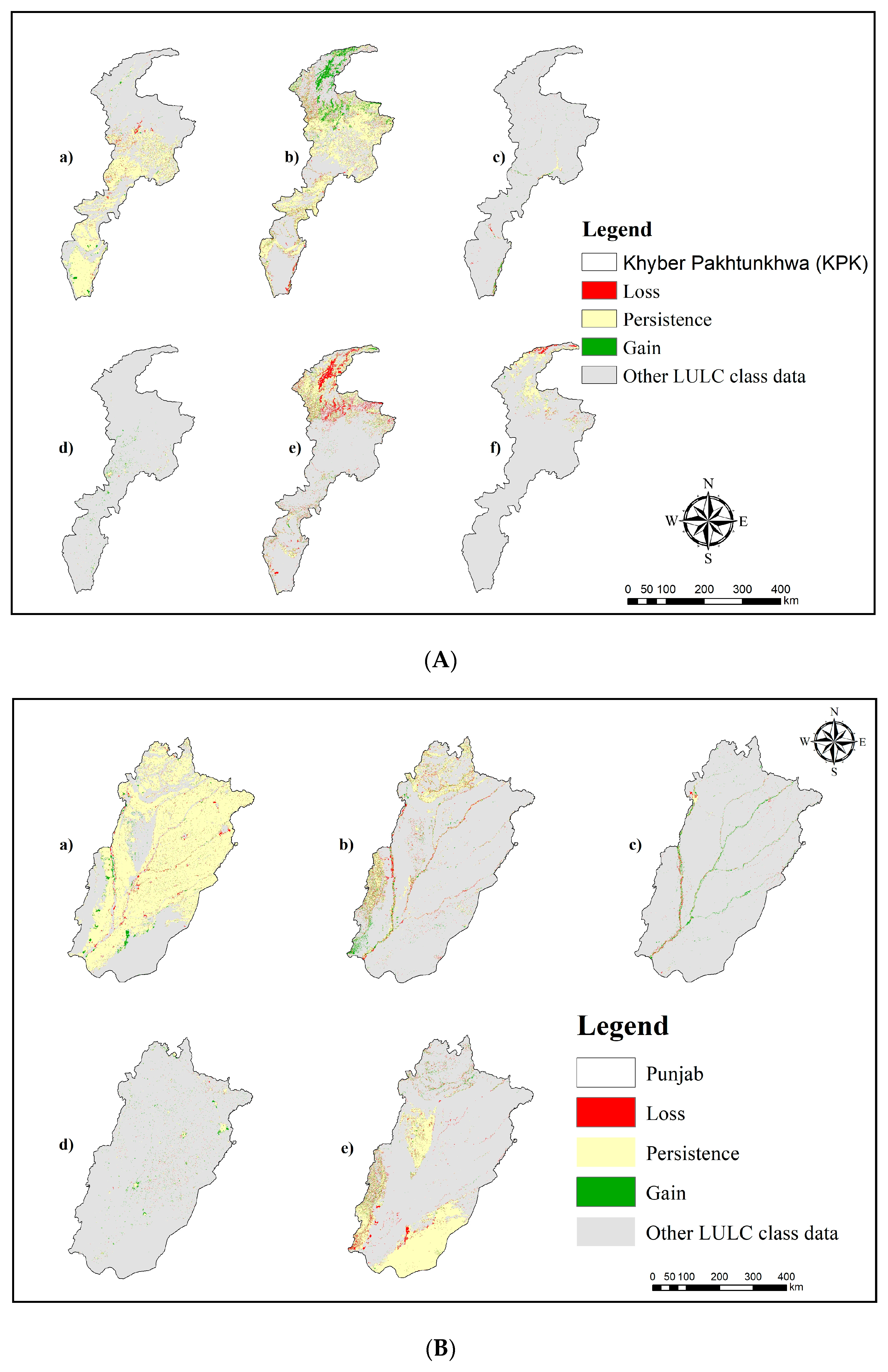
3.1.2. Gain and Loss between LULC Classes over the Period 2000–2020

We employed a “Land Change modeler (LCM) for ecological sustainability” after assessing LULC trends, transitions, and probabilities to pinpoint precisely where the LULC shifts will occur (TerrSet 2020). Results are presented in Figure 5A,B (Provisional Scenarios), and Figure 5C (sample sites) for the last two decades.

Analysis indicated a significant change in the vegetation and barren land for KPK province, where a total of 4375.87 sq. km area was changed from bare land to vegetation (Table 3). Further results for the sample sites (a, b, and c) in Figure 5C indicate significant gains for vegetation cover of 5716.6 km² and 506.9 km² for artificial surfaces, mainly coming from the apparent loss of bare land of 2035 km² (Table S4, Supplementary Materials). This also supports and validates our above results about the spatial patterns of LULC and transitions over KPK province.

In contrast, for the Punjab province, a significant loss was observed in both vegetation (−4592.4 km²) and bare land (−4352.6 km²), with a gain in artificial surfaces (1757.6 km²). This also validated our transitions and probabilities analysis; similar trends were observed over site (c) Lahore, with a significant loss of bare land and vegetation land and substantial gain in artificial surfaces (Table S5 in the Supplementary Materials). Meanwhile, the scenarios (Figure 5C) highlighted apparent improvements in vegetation area over the sample sites (a) and (b). In contrast, site (c) indicated a significant loss of bare land and green fraction cover with a dominant gain in artificial surfaces.

3.2. Land Surface Temperature (LST) Variations

Spatial patterns of the monthly (March-June) mean LST (Figure 6) indicated a significant decrease of −4.3 °C from 2000–2020 over sites (a) and (b). The fluctuation in the LST (increase/decrease) was dominant over the areas of green fraction transitions. Several studies have already indicated the vegetation fraction in this phenomenon [86,87,88,89,90,91,92]. Over sites (a) and (b), apparent changes can be observed, especially after 2010 in (a3) and (b3) when they increased their vegetation cover under the BTTP, as compared to (a1) and (b1) for both high and low LST. On the other hand, site (c) indicated an opposite trend, with an increase of 5.3 °C from 2000–2020, with a significant fluctuation over the central and southern parts, where it lost the green fraction cover (Figure 5C).

3.3. Spatial Patterns of Normalized Difference Vegetation Index (NDVI)

To further analyze the relationship between LST and NDVI, we calculated the spatial patterns of NDVI (Figure 7) to build a linear regression between LST and NDVI (Figure 8;

Table 4. Linear regression analysis over the sites (a, b, and c).

Peshawar	Equation	y = a + b × x	y = a + b × x	y = a + b × x
	Plot	NDVI 2000	NDVI 2010	NDVI 2020
	Weight	No Weighting	No Weighting	No Weighting
	Intercept	1.20 ± 0.01	1.92479 ± 0.02	1.89 ± 0.02
	Slope	−0.03 ± 4.24	−0.06 ± 0.00	−0.06 ± 8.20
	Residual sum of squares	4.74	5.56	6.27
	Pearson’s r	−0.88	−0.83	−0.89
	R2 (COD)/	0.78	0.70	0.80
Swat	Equation	y = a + b × x	y = a + b × x	y = a + b × x
	Plot	NDVI 2000	NDVI 2010	NDVI 2020
	Weight	No Weighting	No Weighting	No Weighting
	Intercept	1.38 ± 0.02	2.02 ± 0.03	1.70 ± 0.04
	Slope	−0.04 ± 9.85	−0.06 ± 0.00	−0.05 ± 0.00
	Residual sum of squares	2.88	3.80	4.43
	Pearson’s r	−0.78	−0.83	−0.68
	R2 (COD)	0.58	0.61	0.69
Lahore	Equation	y = a + b × x	y = a + b × x	y = a + b × x
	Plot	NDVI 2000	NDVI 2010	NDVI 2020
	Weight	No Weighting	No Weighting	No Weighting
	Intercept	1.99 ± 0.02	1.32 ± 0.02	0.77 ± 0.01
	Slope	−0.07 ± 8.53	−0.04 ± 8.42	−0.02 ± 3.32
	Residual sum of squares	3.35	1.66	0.75
	Pearson’s r	−0.89	−0.84	−0.84
	R2 (COD)	0.83	0.72	0.59

) over the sites (a, b, and c).

Correlation statistics revealed a strong relationship for sites (a) and (c) with overall values of 0.70 or above for R² (Table 4). For site (c) Lahore, a decreasing trend for NDVI produced R² values of (c1) 0.83, (c2) 0.72, and (c3) 0.59, with a significant decrease over the central and southern parts of the area. Similarly, for sites (a) Peshawar and (b) Swat, an increasing trend and strong correlation was found for the R² at (a1) 0.78, (a2) 0.70, (a3) 0.84, (b1) 0.58, (b2) 0.61, and (b3) 0.69.

3.4. Relationship between LULC Transitions and LST

After evaluating the relationship between NDVI and LST, we further analyzed the impacts of LULC transitions on LST (

Table 5. CFLRM-based average contribution rate of LULC class transition to LST (°C) from 2000 to 2020.

		Cultivated Land	Vegetation	Water Bodies	Artificial Surfaces	Bare Land	Permanent Snow and Ice
Peshawar	Cultivated land	−0.01	−0.05	0.07	0.11	0.16	NA
	Vegetation	0.03	−0.01	0.06	0.18	0.13	−0.1
	Water bodies	−0.2	−0.13	0.01	0.14	0.17	0.1
	Artificial surfaces	−0.18	−0.15	−0.1	0.01	0.09	NA
	Bare land	−0.08	−0.24	−0.1	0.12	0.01	−0.14
Swat	Cultivated land	−0.02	−0.04	0.05	0.09	0.14	−0.01
	Vegetation	0.02	−0.02	0.04	0.13	0.16	−0.03
	Water bodies	0.1	0.06	0.02	0.1	0.15	−0.1
	Artificial surfaces	−0.12	0.16	−0.2	0	0.1	−0.09
	Bare land	−0.05	−0.19	−0.02	0.14	0	−0.17
Lahore	Cultivated land	−0.01	−0.03	0.1	0.13	0.14	NA
	Vegetation	0.02	−0.01	−0.09	0.17	0.16	NA
	Water	−0.02	0.06	0.1	0.13	0.14	NA
	Artificial surfaces	−0.19	−0.21	−0.11	0.19	0.17	NA
	Bare land	−0.22	−0.18	−0.01	0.16	0.06	NA

NA = Not applicable.

) using CFLRM. Results from Table 5 indicated a decreasing trend for LST over the LULC classes associated with land transformation from bare or built-up land to vegetation and cultivated land. Over site (c), a significant gain of LST (0.17 °C) was noted in response to the transformation of VG to BU. In contrast, substantial reductions were seen in LST (−0.21 °C) after transition from built-up land/artificial surfaces (BU) to vegetation (VG), (−0.19 °C) after transition from BU to CL (cultivated land), and (−0.22 °C) after transition from bare land (BR) to CL.

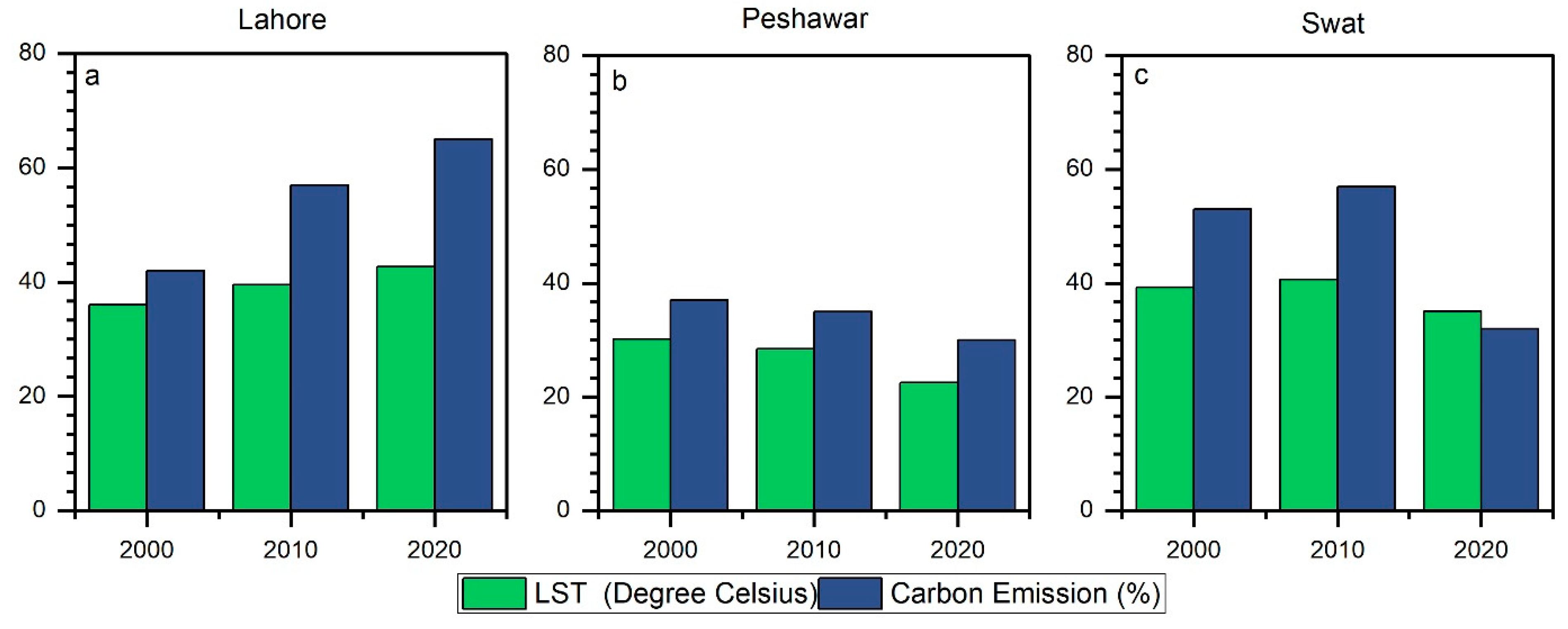
3.5. Carbon Stock Maps and Analysis between Carbon Emission and LST

Using the CFLRM, we analyzed the scenarios of land cover dynamics and LULC transitions, including the geographical locations of gain and loss, variations in LST throughout the research period, and the contribution rates of LULC transitions to LST.

The results shown in Figure 9 indicated low carbon stock over bare land/water, medium over built-up land, and high stock over vegetation-covered areas, which were in line with previous studies in this domain [93,94,95,96]. Furthermore, the sensitivity analysis [29] of the relationship between LST and CO₂ variation (%), shown in Figure 10, indicated that CO₂ emission variation (%) was highly sensitive to LST. Results suggested that fluctuations in LST are affecting the % of emission. Over Lahore, we noticed a growing LST and a corresponding increase in the percent of CO₂ flux. In contrast, the study indicated a decreasing LST and a definite drop in the percentage of CO₂ variation over Peshawar and Swat. Studies have highlighted the fact that green fraction cover fluctuation affects the LST and the CE, as a decrease in vegetation fraction results in a massive reduction of carbon sink from the environment and traps CO₂ in the atmosphere, which also contributes to fluctuations in the LST [97,98,99,100,101,102,103,104].

4. Discussion

This research was carried out to monitor and compare scenarios of land cover dynamics from 2000–2020 associated with the different land-use policies of local governments and to analyze their impacts on LST in the Punjab and KPK provinces of Pakistan. Furthermore, carbon stock maps were prepared, and the linkage between CE and LST was explored. Findings indicated a significant increase in artificial surfaces over KPK from 664.18 km² in 2000 to 1196.17 km² in 2010 and 1375.82 km² in 2020. A significant part of the increase in artificial surfaces was due to the mass migration of people from Afghanistan toward the KPK [105]. In addition, the same trends were observed over Punjab province and site “c”, where a significant increase in artificial surfaces from 3846.3 km² in 2000 to 4065.38 km² in 2010 and 6497.6 km² by 2020 were noted. This was mainly because of the development of new housing communities in response to a growing urban population [50,51], mega-development projects (including Metro Bus, Orange Train) [50,51,106], and the RUDP (designed for up to approximately 35 million inhabitants and using an area of 40,000 ha). Furthermore, our results indicated that the increase in artificial surfaces was mainly at the cost of losing green fraction, which is essential for equilibrium between the land surface and atmospheric parameters [66,107]. An increase in population required new commercial and residential areas, as well as public utilities and transportation infrastructure, which also caused a decrease in green vegetation [108,109].

Previous studies [53,64,110,111,112,113] also reported that transitions in LULC, especially an increase in artificial surfaces, affect the LST and carbon emission and profoundly impact local and regional climates. As a result of variations in surface roughness and reflectance among the LULC categories, the amount of energy radiated and absorbed by these objects can vary significantly [21,22]. Our study explored these conclusions by evaluating the spatio-temporal changes in LST associated with the historical transitions of each LULC category. We concluded that there was a significant decrease in LST by 4.3 °C from 2000–2020 over sites (a) and (b), while an increase of 5.3 °C over site (c) was observed. To further understand the relationship of LST with vegetation cover, we utilized the linear regression between LST and NDVI [87,92] and found a strong positive correlation. Results indicated a significant gain in LST (0.17 °C) in response to the transformation of VG to BU. In contrast, there was a significant decrease in LST (−0.21 °C) over the transition from built-up land/artificial surfaces (BU) to vegetation (VG), (−0.19 °C) over the transition from BU to CL (cultivated land), and (−0.22 °C) over the transition from bare land (BR) to CL was noted.

The decreasing trend of LST can be seen after 2010, when the provisional government initialized the BTTP project to minimize the effects of green fraction loss [64], and then achieved its goals in 2017 [65]. Several pieces of research have already indicated the importance of the vegetation fraction in this phenomenon; e.g., [86] reported that safeguarding biodiversity and vegetation such as forests, agricultural land, and dense or sparse vegetation, is necessary to maintain the soil cover and balance in the ecosystem, hydrological cycle, surface temperatures, and air because each land-use category has a different magnitude of surface reflectance and roughness [114,115]. Research findings indicated that in response to the increase in vegetation land under the BTTP, the LST of the area saw a decreasing trend. In contrast, Lahore, in the Punjab province of Pakistan, has shown a decreasing trend for vegetation and an increasing trend for artificial surfaces since 2000, which significantly alter the LST and carbon emission [98,101,102,103,104].

We next examined the carbon stock and carbon emission over the research region after determining the LULC dynamics, LST pattern, and the contribution rate of each LULC transition on LST. Several studies [97,98,99,100] have reported that transitions in LULC, especially the loss/gain of green fraction, impact the LST, carbon stocks, and CE [93,94,95,96]. Our results indicated low carbon stock over bare land/water, medium over built-up land, and high stock over vegetation-covered areas. Kafy et al. [29] also reported the same results in Bangladesh. Green portion conversion to high-rise infrastructure boosts carbon emissions [27]. The primary driver of carbon emissions is the expansion of artificial surfaces [116], which has been a primary concern since the industrial revolution [26]. Updated LULC information is essential for understanding environmental pressures such as carbon emissions, biosafety, resource depletion, and climate change [9,117,118], and it is crucial for mesoscale dynamic understanding [119,120,121]. For example, climate models specify that the Paris Agreement’s purpose can be achieved by efficient and sustainable policies relating to low carbon emissions [46,52]. Depleting carbon levels can be reduced through artificial adjustments of land cover patterns [53,54].

5. Conclusions

The study findings confirmed that over the study period, the KPK province, along with sites (a) Peshawar and (b) Swat, was predominantly gaining vegetation cover by +5.35%. A 1.13% increase was noted between 2000–2010, but the ratio accelerated to +4.16% from 2010–2020 under the BTTP project with an effective transition of bare land totalling 4375.87 km² to vegetation. On the other hand, the scenarios were alarming for the Punjab province, along with site (c) Lahore, where there was an increase in artificial surfaces from 1.83% in 2000 to 3.10% in 2020 at the cost of vegetation and bare land loss, amounting to a significant transition of 1074.9 km² of vegetation land and 1840.3 km² of bare ground to artificial surfaces. Shifts in LULC can alter LST. This study reported an increase of 5.3 °C LST over Lahore, Punjab, whereas a significant drop in LST by −4.3 °C was detected over KPK province. Furthermore, a significant association was found between the LST and NDVI with R² > 0.70.

The contribution rate of LULC transitions to LST suggested a considerable influence of land cover transitions on LST, with a 0.17 °C increase seen across regions transformed from vegetation to artificial surfaces, whereas there was an effective decrease of −0.21 °C in LST over artificial surfaces transformed to vegetation, −0.19 °C over artificial surfaces transformed to cultivated land, and −0.22 °C over bare land transformed to cultivated land. The results for carbon stock indicated a low carbon stock over bare land/water, medium over built-up land, and high stock over the vegetation-covered areas for both Punjab and KPK provinces. The sensitivity analysis between LST and carbon emission indicated that CO₂ emission variation (%) was highly sensitive to LST. The results suggested that fluctuations in LST are affecting the % of emission.

The research indicated that the boost in vegetation cover at the cost of bare land in response to the BTTP project produced a positive and robust environmental impact. On the other hand, the site (c) scenarios indicated dangerous trends which not only assisted in increasing LST but also caused a high carbon emission rate. The findings of this research and several previous studies have already highlighted the importance of vegetation fraction for the urban environment and the consequences of rapid urban development. Therefore, the government of Punjab should revisit its LULC policies, especially, in the context of the Master Plan 2050, the plans to build a new city (RUDP) adjacent to site (c) by acquiring farming land and transforming it into artificial surfaces, which would accelerate the negative consequences for the environment and local communities. Instead of converting farmland to artificial surfaces, authorities might follow KPK’s policies (e.g., the BTTP) to boost the green proportion.

References

1. Al Rakib, A.; Akter, K.S.; Rahman, M.N.; Arpi, S.; Kafy, A.A. Analyzing the pattern of land use land cover change and its impact on land surface temperature: A remote sensing approach in Mymensingh, Bangladesh. In Proceedings of the 1st International Student Research Conference-2020, Dhaka, Bangladesh, 1 April 2020. [Google Scholar]
2. Nurwanda, A.; Honjo, T. The prediction of city expansion and land surface temperature in Bogor City, Indonesia. Sustain. Cities Soc. 2019, 52, 101772. [Google Scholar] [CrossRef]
3. Omar, N.Q.; Sanusi, S.A.M.; Hussin, W.M.W.; Samat, N.; Mohammed, K.S. Markov-CA model using analytical hierarchy process and multiregression technique. In Proceedings of the IOP Conference Series: Earth and Environmental Science, Kuala Lumpur, Malaysia, 22–23 April 2014. [Google Scholar]
4. Chen, X.-L.; Zhao, H.-M.; Li, P.-X.; Yin, Z.-Y. Remote sensing image-based analysis of the relationship between urban heat island and land use/cover changes. Remote Sens. Environ. 2006, 104, 133–146. [Google Scholar] [CrossRef]
5. Mitchell, L.; Moss, H.O.N. Urban Mobility in the 1st Century; NYU Rudin Center for Transportation Policy: New York, NY, USA, 2012. [Google Scholar]
6. Mumtaz, F.; Tao, Y.; de Leeuw, G.; Zhao, L.; Fan, C.; Elnashar, A.; Bashir, B.; Wang, G.; Li, L.; Naeem, S.; et al. Modeling Spatio-Temporal Land Transformation and Its Associated Impacts on land Surface Temperature (LST). Remote Sens. 2020, 12, 2987. [Google Scholar] [CrossRef]
7. Bank, T.W. Urban Population. 2018. Available online: https://data.worldbank.org/indicator/SP.URB.TOTL.IN.ZS/ (accessed on 2 June 2022).
8. De Sherbinin, A. A CIESIN Thematic Guide to Land-Use and Land-Cover Change (LUCC); Center for International Earth Science Information Network, Columbia University: New York, NY, USA, 2002. [Google Scholar]
9. Eastman, J.; Van Fossen, M.; Solarzano, L. Transition Potential Modeling for Land Cover Change; GIS, Spatial Analysis and Modeling; ESRI Press: Redlands, CA, USA, 2005; pp. 357–386. [Google Scholar]
10. Rai, R.; Zhang, Y.; Paudel, B.; Li, S.; Khanal, N.R. A Synthesis of Studies on Land Use and Land Cover Dynamics during 1930–2015 in Bangladesh. Sustainability 2017, 9, 1866. [Google Scholar] [CrossRef]
11. Briassoulis, H. Analysis of Land Use Change: Theoretical and Modeling Approaches; University of the Aegean: Mitilini, Greece, 2020. [Google Scholar]
12. Lin, Y.; Qiu, R.; Yao, J.; Hu, X.; Lin, J. The effects of urbanization on China’s forest loss from 2000 to 2012: Evidence from a panel analysis. J. Clean. Prod. 2019, 214, 270–278. [Google Scholar] [CrossRef]
13. Wang, Z.-H. Reconceptualizing urban heat island: Beyond the urban-rural dichotomy. Sustain. Cities Soc. 2021, 77, 103581. [Google Scholar] [CrossRef]
14. Dubovyk, O.; Sliuzas, R.; Flacke, J. Spatio-temporal modelling of informal settlement development in Sancaktepe district, Istanbul, Turkey. ISPRS J. Photogramm. Remote Sens. 2011, 66, 235–246. [Google Scholar] [CrossRef]
15. Poelmans, L.; Van Rompaey, A. Detecting and modelling spatial patterns of urban sprawl in highly fragmented areas: A case study in the Flanders–Brussels region. Landsc. Urban Plan. 2009, 93, 10–19. [Google Scholar] [CrossRef]
16. Song, X.; Zeng, X. Evaluating the responses of forest ecosystems to climate change and CO2 using dynamic global vegetation models. Ecol. Evol. 2017, 7, 997–1008. [Google Scholar] [CrossRef] [PubMed]
17. Bowman, D.M.J.S.; Kolden, C.A.; Abatzoglou, J.T.; Johnston, F.H.; van der Werf, G.R.; Flannigan, M. Vegetation fires in the Anthropocene. Nat. Rev. Earth Environ. 2020, 1, 500–515. [Google Scholar] [CrossRef]
18. Gidado, K.A.; Kamarudin, M.K.A.; Firdausaq, N.A.; Nalado, A.M.; Saudi, A.S.M.; Saad, M.H.; Ibrahim, S. Analysis of Spatiotemporal Land Use and Land Cover Changes using Remote Sensing and GIS: A Review. Int. J. Eng. Technol. 2018, 7, 159–162. [Google Scholar] [CrossRef]
19. Waseem, S.; Khayyam, U. Loss of vegetative cover and increased land surface temperature: A case study of Islamabad, Pakistan. J. Clean. Prod. 2019, 234, 972–983. [Google Scholar] [CrossRef]
20. Tang, X.; Woodcock, C.E.; Olofsson, P.; Hutyra, L.R. Spatiotemporal assessment of land use/land cover change and associated carbon emissions and uptake in the Mekong River Basin. Remote Sens. Environ. 2021, 256, 112336. [Google Scholar] [CrossRef]
21. Ahmad, A.; Nizami, S.M. Carbon stocks of different land uses in the Kumrat valley, Hindu Kush Region of Pakistan. J. For. Res. 2015, 26, 57–64. [Google Scholar] [CrossRef]
22. Abutaleb, K.; Ngie, A.; Darwish, A.; Ahmed, M.; Arafat, S.; Ahmed, F. Assessment of Urban Heat Island Using Remotely Sensed Imagery over Greater Cairo, Egypt. Adv. Remote Sens. 2015, 04, 35–47. [Google Scholar] [CrossRef]
23. Canadell, J.G.; Raupach, M.R. Managing Forests for Climate Change Mitigation. Science 2008, 320, 1456–1457. [Google Scholar] [CrossRef]
24. Mackey, B. Counting trees, carbon and climate change. Significance 2014, 11, 19–23. [Google Scholar] [CrossRef]
25. Penman, J.; Gytarsky, M.; Hiraishi, T.; Krug, T.; Kruger, D.; Pipatti, R.; Buendia, L.; Miwa, K.; Ngara, T.; Tanabe, K.; et al. Good Practice Guidance for Land Use, Land-Use Change and Forestry. 2003. Available online: https://www.ipcc-nggip.iges.or.jp/public/gpglulucf/gpglulucf_files/GPG_LULUCF_FULL.pdf (accessed on 2 June 2022).
26. Houghton, R.A.; House, J.I.; Pongratz, J.; Van Der Werf, G.R.; DeFries, R.S.; Hansen, M.C.; Le Quéré, C.; Ramankutty, N. Carbon emissions from land use and land-cover change. Biogeosciences 2012, 9, 5125–5142. [Google Scholar] [CrossRef]
27. Chuai, X.; Huang, X.; Wang, W.; Zhao, R.; Zhang, M.; Wu, C. Land use, total carbon emission’s change and low carbon land management in Coastal Jiangsu, China. J. Clean. Prod. 2015, 103, 77–86. [Google Scholar] [CrossRef]
28. Djalante, R. Key assessments from the IPCC special report on global warming of 1.5 C and the implications for the Sendai framework for disaster risk reduction. Prog. Disaster Sci. 2019, 1, 100001. [Google Scholar] [CrossRef]
29. Kafy, A.A.; Al Rakib, A.; Fattah, M.A.; Rahaman, Z.A.; Sattar, G.S. Impact of vegetation cover loss on surface temperature and carbon emission in a fastest-growing city, Cumilla, Bangladesh. Build. Environ. 2022, 208, 108573. [Google Scholar] [CrossRef]
30. Mumtaz, F.; Arshad, A.; Mirchi, A.; Tariq, A.; Dilawar, A.; Hussain, S.; Shi, S.; Noor, R.; Noor, R.; Daccache, A.; et al. Impacts of reduced deposition of atmospheric nitrogen on coastal marine eco-system during substantial shift in human activities in the twenty-first century. Geomatics, Nat. Hazards Risk 2021, 12, 2023–2047. [Google Scholar] [CrossRef]
31. Jayakrishnan, K.U.; Bala, G.; Cao, L.; Caldeira, K. Contrasting climate and carbon-cycle consequences of fossil-fuel use versus deforestation disturbance. Environ. Res. Lett. 2022, 17, 064020. [Google Scholar] [CrossRef]
32. Fang, J.; Guo, Z.; Piao, S.; Chen, A. Terrestrial vegetation carbon sinks in China, 1981–2000. Sci. China Ser. D Earth Sci. 2007, 50, 1341–1350. [Google Scholar] [CrossRef]
33. Pilli, R.; Grassi, G. Bilancio del carbonio negli ecosistemi terrestri cinesi. For.-J. Silvic. For. Ecol. 2009, 6, 137. [Google Scholar]
34. Pan, G.; Li, L.; Wu, L.; Zhang, X. Storage and sequestration potential of topsoil organic carbon in China’s paddy soils. Glob. Chang. Biol. 2004, 10, 79–92. [Google Scholar] [CrossRef]
35. Zhang, G.; Kang, Y.; Han, G.; Mei, H.; Sakurai, K. Grassland degradation reduces the carbon sequestration capacity of the vegetation and enhances the soil carbon and nitrogen loss. Acta Agric. Scand. Sect. B—Soil Plant Sci. 2011, 61, 356–364. [Google Scholar] [CrossRef]
36. DeFries, R.S.; Houghton, R.A.; Hansen, M.C.; Field, C.B.; Skole, D.; Townshend, J. Carbon emissions from tropical deforestation and regrowth based on satellite observations for the 1980s and 1990s. Proc. Natl. Acad. Sci. USA 2002, 99, 14256–14261. [Google Scholar] [CrossRef]
37. Houghton, R. Magnitude, distribution and causes of terrestrial carbon sinks and some implications for policy. Clim. Policy 2002, 2, 71–88. [Google Scholar] [CrossRef]
38. Leite, C.C.; Costa, M.H.; Soares-Filho, B.S.; Hissa, L.D.B.V. Historical land use change and associated carbon emissions in Brazil from 1940 to 1995. Glob. Biogeochem. Cycles 2012, 26. [Google Scholar] [CrossRef]
39. FAO; UN. Global Forest Resources Assessment 2020: Key Findings; FAO: Rome, Italy, 2020. [Google Scholar]
40. NOAA. NOAA’s Greenhouse Gas Index Up 41 Percent Since 1990. 2018. Available online: https://research.noaa.gov/article/ArtMID/587/ArticleID/2359/NOAA%E2%80%99s-greenhouse-gas-index-up-41-percent-since-1990 (accessed on 2 June 2022).
41. Tiseo, I. Historic Average Carbon Dioxide (CO2) Levels in the Atmosphere Worldwide from 1959 to 2021 (in Parts Per Million). 2021. Available online: https://www.statista.com/statistics/1091926/atmospheric-concentration-of-co2-historic/ (accessed on 18 November 2022).
42. Wang, G.; Zhang, L.; Zhuang, Q.; Yu, D.; Shi, X.; Xing, S.; Xiong, D.; Liu, Y. Quantification of the soil organic carbon balance in the Tai-Lake paddy soils of China. Soil Tillage Res. 2016, 155, 95–106. [Google Scholar] [CrossRef]
43. IPCC (Intergovernmental Panel on Climate Change). Synthesis Report. Summary for Policymakers; Cambridge University Press: Cambridge, UK, 2007. [Google Scholar]
44. World Bank Data Team. The 2017 Atlas of Sustainable Development Goals: A New Visual Guide to Data and Development. 2017. Available online: https://blogs.worldbank.org/opendata/2017-atlas-sustainable-development-goals-new-visual-guide-data-and-development (accessed on 18 November 2022).
45. The Intergovernmental Panel on Climate Change (IPCC). Climate Change 2021—The Physical Science Basis in AR6. 2021. Available online: https://www.ipcc.ch/report/ar6/wg1/ (accessed on 18 November 2022).
46. Tollefson, J. The 2 C Dream. Nature 2015, 527, 436. [Google Scholar] [CrossRef] [PubMed]
47. Dixon, R.K.; Solomon, A.M.; Brown, S.; Houghton, R.A.; Trexier, M.C.; Wisniewski, J. Carbon Pools and Flux of Global Forest Ecosystems. Science 1994, 263, 185–190. [Google Scholar] [CrossRef] [PubMed]
48. Houghton, R.A.; Hackler, J.L. Emissions of carbon from forestry and land-use change in tropical Asia. Glob. Chang. Biol. 1999, 5, 481–492. [Google Scholar] [CrossRef]
49. Houghton, R.A.; Nassikas, A.A. Global and regional fluxes of carbon from land use and land cover change 1850–2015. Glob. Biogeochem. Cycles 2017, 31, 456–472. [Google Scholar] [CrossRef]
50. Han, J.; Meng, X.; Zhou, X.; Yi, B.; Liu, M.; Xiang, W.N. A long-term analysis of urbanization process, landscape change, and carbon sources and sinks: A case study in China’s Yangtze River Delta region. J. Clean. Prod. 2017, 141, 1040–1050. [Google Scholar] [CrossRef]
51. Shevliakova, E.; Pacala, S.W.; Malyshev, S.; Hurtt, G.C.; Milly, P.C.D.; Caspersen, J.P.; Sentman, L.T.; Fisk, J.P.; Wirth, C.; Crevoisier, C. Carbon cycling under 300 years of land use change: Importance of the secondary vegetation sink. Glob. Biogeochem. Cycles 2009, 23. [Google Scholar] [CrossRef]
52. Zhu, E.; Deng, J.; Zhou, M.; Gan, M.; Jiang, R.; Wang, K.; Shahtahmassebi, A. Carbon emissions induced by land-use and land-cover change from 1970 to 2010 in Zhejiang, China. Sci. Total. Environ. 2019, 646, 930–939. [Google Scholar] [CrossRef]
53. Lal, R. Forest soils and carbon sequestration. For. Ecol. Manag. 2005, 220, 242–2588. [Google Scholar] [CrossRef]
54. Guadalupe, V.; Sotta, E.D.; Santos, V.F.; Aguiar, L.J.G.; Vieira, M.; de Oliveira, C.P.; Siqueira, J.V.N. REDD+ implementation in a high forest low deforestation area: Constraints on monitoring forest carbon emissions. Land Use Policy 2018, 76, 414–421. [Google Scholar] [CrossRef]
55. Wulder, M.A.; White, J.C.; Loveland, T.R.; Woodcock, C.E.; Belward, A.S.; Cohen, W.B.; Fosnight, E.A.; Shaw, J.; Masek, J.G.; Roy, D.P. The global Landsat archive: Status, consolidation, and direction. Remote Sens. Environ. 2016, 185, 271–283. [Google Scholar] [CrossRef] [Green Version]
56. Du, L.; Zhou, T.; Zou, Z.; Zhao, X.; Huang, K.; Wu, H. Mapping Forest Biomass Using Remote Sensing and National Forest Inventory in China. Forests 2014, 5, 1267–1283. [Google Scholar] [CrossRef]
57. Balcik, F.B.; Kuzucu, A.K. Determination of Land Cover/Land Use Using SPOT 7 Data With Supervised Classification Methods. In Proceedings of the 3rd International GeoAdvances Workshop, Istanbul, Turkey, 16–17 October 2016; pp. 143–146. [Google Scholar]
58. Mitchell, A.L.; Rosenqvist, A.; Mora, B. Current remote sensing approaches to monitoring forest degradation in support of countries measurement, reporting and verification (MRV) systems for REDD+. Carbon Balance Manag. 2017, 12, 1–22. [Google Scholar] [CrossRef] [PubMed]
59. Eckstein, A.; Künzel, V.; Schäfer, L. Global Climate Risk Index 2021. In Who Suffers Most from Extreme Weather Events? Weather-Related Loss Events in 2019 and 2000–2019; Germanwatch e.V.: Bonn, Germany, 2021; ISBN 978-3-943704-84-6. [Google Scholar]
60. Khan, W.R.; Khokhar, M.F.; Sana, M.; Naila, Y.; Qurban, A.P.; Muhammad, N.R. Assessing the context of REDD+ in Murree hills forest of Pakistan. Adv. Environ. Biol. 2015, 9, 15–20. [Google Scholar]
61. Munawar, S.; Khokhar, M.F.; Atif, S. Reducing emissions from deforestation and forest degradation implementation in northern Pakistan. Int. Biodeterior. Biodegrad. 2015, 102, 316–323. [Google Scholar] [CrossRef]
62. Yasmin, N. Dynamical Assessment of Vegetation Trends over Margalla Hills National Park by Using Modis Vegetation Indices. Pak. J. Agric. Sci. 2016, 53, 777–786. [Google Scholar]
63. ICIMOD. The REDD+ Project in Pakistan. 2013. Available online: https://redd.unfccc.int/files/pakistan_redd__strategy_final-oct_2_2021_edited_by_iucn-new_minister.pdf (accessed on 18 November 2022).
64. UNESCO. Pakistan: Green Again. 2019. Available online: https://en.unesco.org/courier/2019-3/pakistan-green-again (accessed on 18 November 2022).
65. WEF. Pakistan Has Planted over a Billion Trees. 2018. Available online: https://www.weforum.org/agenda/2018/07/pakistan-s-billion-tree-tsunami-is-astonishing/ (accessed on 18 November 2022).
66. Rana, I.A.; Bhatti, S.S. Lahore, Pakistan–Urbanization challenges and opportunities. Cities 2018, 72, 348–355. [Google Scholar] [CrossRef]
67. Shah, B.; Ghauri, B. Mapping urban heat island effect in comparison with the land use, land cover of Lahore district. Pak. J. Meteorol. Vol 2015, 11, 37–48. [Google Scholar]
68. Nespak, L. Integrated Master Plan for Lahore-2021; Lahore Development Authority: Lahore, Pakistan, 2004. [Google Scholar]
69. Baloch, S.M. We Will be Homeless’: Lahore Farmers Accuse ‘Mafia’ of Land Grab for New City. 2021. Available online: https://www.theguardian.com/global-development/2021/nov/02/we-will-be-homeless-lahore-farmers-accuse-mafia-of-land-grab-for-new-city (accessed on 18 November 2022).
70. Xu, Z.; Luo, Q.; Xu, Z. Consistency of land cover data derived from remote sensing in Xinjiang. J. Geo-Inf. Sci. 2019, 21, 427–436. [Google Scholar]
71. Hou, W.; Hou, X. Consistency of the multiple remote sensing-based land use and land cover classification products in the global coastal zones. J. Geo-Inf. Sci. 2019, 21, 1061–1073. [Google Scholar]
72. Shi, X.; Nie, S.; Ju, W.; Yu, L. Climate effects of the GlobeLand30 land cover dataset on the Beijing Climate Center climate model simulations. Sci. China Earth Sci. 2016, 59, 1754–1764. [Google Scholar] [CrossRef]
73. Tariq, A.; Shu, H. CA-Markov Chain Analysis of Seasonal Land Surface Temperature and Land Use Land Cover Change Using Optical Multi-Temporal Satellite Data of Faisalabad, Pakistan. Remote Sens. 2020, 12, 3402. [Google Scholar] [CrossRef]
74. Kumar, S.; Radhakrishnan, N.; Mathew, S. Land use change modelling using a Markov model and remote sensing. Geomat. Nat. Hazards Risk 2013, 5, 145–156. [Google Scholar] [CrossRef]
75. Qin, Z.; Dall’Olmo, G.; Karnieli, A.; Berliner, P. Derivation of split window algorithm and its sensitivity analysis for retrieving land surface temperature from NOAA-advanced very high resolution radiometer data. J. Geophys. Res. Atmos. 2001, 106, 22655–22670. [Google Scholar] [CrossRef]
76. Jimenez-Munoz, J.C.; Cristobal, J.; Sobrino, J.A.; Soria, G.; Ninyerola, M.; Pons, X. Revision of the Single-Channel Algorithm for Land Surface Temperature Retrieval From Landsat Thermal-Infrared Data. IEEE Trans. Geosci. Remote Sens. 2008, 47, 339–349. [Google Scholar] [CrossRef]
77. Abuelgasim, A.; Ammad, R. Mapping soil salinity in arid and semi-arid regions using Landsat 8 OLI satellite data. Remote Sens. Appl. Soc. Environ. 2019, 13, 415–425. [Google Scholar] [CrossRef]
78. Onačillová, K.; Gallay, M.; Paluba, D.; Péliová, A.; Tokarčík, O.; Laubertová, D. Combining Landsat 8 and Sentinel-2 Data in Google Earth Engine to Derive Higher Resolution Land Surface Temperature Maps in Urban Environment. Remote Sens. 2022, 14, 4076. [Google Scholar] [CrossRef]
79. USGS. Curve Fit Linear Regression. 2017. Available online: https://www.usgs.gov/centers/upper-midwest-environmental-sciences-center/science/curve-fit-pixel-level-raster-regression# (accessed on 18 November 2022).
80. Nizami, S.M. The inventory of the carbon stocks in sub tropical forests of Pakistan for reporting under Kyoto Protocol. J. For. Res. 2012, 23, 377–384. [Google Scholar] [CrossRef]
81. Afzal, M.; Akhter, A. Estimation of biomass and carbon stock: Chichawatni Irrigated Plantation in Punjab, Pakistan. In Proceedings of the SDPI’s Fourteenth Sustainable Development Conference, Islamabad, Pakistan, 13–15 December 2011. [Google Scholar]
82. Pearson, T.; Walker, S.; Brown, S. Sourcebook for Land Use, Land-Use Change and Forestry Projects; World Bank: Washington, DC, USA, 2013. [Google Scholar]
83. Chave, J.; Réjou-Méchain, M.; Búrquez, A.; Chidumayo, E.; Colgan, M.S.; Delitti, W.B.; Duque, A.; Eid, T.; Fearnside, P.M.; Goodman, R.C.; et al. Improved allometric models to estimate the aboveground biomass of tropical trees. Glob. Chang. Biol. 2014, 20, 3177–3190. [Google Scholar] [CrossRef] [PubMed]
84. Spawn, S.; Gibbs, H. Global Aboveground and Belowground Biomass Carbon Density Maps for the Year 2010; ORNL DAAC: Oak Ridge, TN, USA, 2020.
85. Spawn, S.A.; Sullivan, C.C.; Lark, T.J.; Gibbs, H.K. Harmonized global maps of above and belowground biomass carbon density in the year 2010. Sci. Data 2020, 7, 1–22. [Google Scholar] [CrossRef]
86. Aljerf, L. Biodiversity is key for More Variety for Better Society. Biodivers. Int. J. 2017, 1, 00002. [Google Scholar] [CrossRef]
87. Guha, S.; Govil, H.; Diwan, P. Monitoring LST-NDVI Relationship Using Premonsoon Landsat Datasets. Adv. Meteorol. 2020, 2020, 1–15. [Google Scholar] [CrossRef]
88. Sun, D.; Kafatos, M. Note on the NDVI-LST relationship and the use of temperature-related drought indices over North America. Geophys. Res. Lett. 2007, 34. [Google Scholar] [CrossRef]
89. Karnieli, A.; Agam, N.; Pinker, R.T.; Anderson, M.; Imhoff, M.L.; Gutman, G.G.; Panov, N.; Goldberg, A. Use of NDVI and Land Surface Temperature for Drought Assessment: Merits and Limitations. J. Clim. 2010, 23, 618–633. [Google Scholar] [CrossRef]
90. Yue, W.; Xu, J.; Tan, W.; Xu, L. The relationship between land surface temperature and NDVI with remote sensing: Application to Shanghai Landsat 7 ETM+ data. Int. J. Remote Sens. 2007, 28, 3205–3226. [Google Scholar] [CrossRef]
91. Marzban, F.; Sodoudi, S.; Preusker, R. The influence of land-cover type on the relationship between NDVI–LST and LST-T air. Int. J. Remote Sens. 2018, 39, 1377–1398. [Google Scholar] [CrossRef]
92. Govil, H.; Guha, S.; Diwan, P.; Gill, N.; Dey, A. Analyzing linear relationships of LST with NDVI and MNDISI using various resolution levels of Landsat 8 OLI and TIRS data. In Data Management, Analytics and Innovation; Springer: Berlin/Heidelberg, Germany, 2020; pp. 171–184. [Google Scholar]
93. Fernandes, M.M.; de Moura Fernandes, M.R.; Garcia, J.R.; Matricardi, E.A.; de Souza Lima, A.H.; de Araújo Filho, R.N.; Gomes Filho, R.R.; Piscoya, V.C.; Piscoya, T.O.; Cunha Filho, M. Land use and land cover changes and carbon stock valuation in the São Francisco river basin, Brazil. Environ. Chall. 2021, 5, 100247. [Google Scholar] [CrossRef]
94. Sohl, T.L.; Sleeter, B.M.; Zhu, Z.; Sayler, K.L.; Bennett, S.; Bouchard, M.; Reker, R.; Hawbaker, T.; Wein, A.; Liu, S.; et al. A land-use and land-cover modeling strategy to support a national assessment of carbon stocks and fluxes. Appl. Geogr. 2012, 34, 111–124. [Google Scholar] [CrossRef]
95. Barakat, A.; Khellouk, R.; Touhami, F. Detection of urban LULC changes and its effect on soil organic carbon stocks: A case study of Béni Mellal City (Morocco). J. Sediment. Environ. 2021, 6, 287–299. [Google Scholar] [CrossRef]
96. Rajbanshi, J.; Das, S. Changes in carbon stocks and its economic valuation under a changing land use pattern—A multitemporal study in Konar catchment, India. Land Degrad. Dev. 2021, 32, 3573–3587. [Google Scholar] [CrossRef]
97. Fattah; Morshed, S.R.; Morshed, S.Y. Multi-layer perceptron-Markov chain-based artificial neural network for modelling future land-specific carbon emission pattern and its influences on surface temperature. SN Appl. Sci. 2021, 3, 1–22. [Google Scholar] [CrossRef]
98. Fattah, A.; Morshed, S.R. Impacts of land use-based carbon emission pattern on surface temperature dynamics: Experience from the urban and suburban areas of Khulna, Bangladesh. Remote Sens. Appl. Soc. Environ. 2021, 22, 100508. [Google Scholar] [CrossRef]
99. Williams, R.G.; Roussenov, V.; Goodwin, P.; Resplandy, L.; Bopp, L. Sensitivity of Global Warming to Carbon Emissions: Effects of Heat and Carbon Uptake in a Suite of Earth System Models. J. Clim. 2017, 30, 9343–9363. [Google Scholar] [CrossRef]
100. Allen, M.R.; Frame, D.J.; Huntingford, C.; Jones, C.D.; Lowe, J.A.; Meinshausen, M.; Meinshausen, N. Warming caused by cumulative carbon emissions towards the trillionth tonne. Nature 2009, 458, 1163–1166. [Google Scholar] [CrossRef] [PubMed]
101. Sleeter, B.M.; Liu, J.; Daniel, C.; Rayfield, B.; Sherba, J.; Hawbaker, T.J.; Zhu, Z.; Selmants, P.C.; Loveland, T.R. Effects of contemporary land-use and land-cover change on the carbon balance of terrestrial ecosystems in the United States. Environ. Res. Lett. 2018, 13, 045006. [Google Scholar] [CrossRef]
102. Sarathchandra, C.; Abebe, Y.A.; Worthy, F.R.; Wijerathne, I.L.; Ma, H.; Yingfeng, B.; Jiayu, G.; Chen, H.; Yan, Q.; Geng, Y.; et al. Impact of land use and land cover changes on carbon storage in rubber dominated tropical Xishuangbanna, South West China. Ecosyst. Heal. Sustain. 2021, 7, 1915183. [Google Scholar] [CrossRef]
103. Yin, K.; Lu, D.; Tian, Y.; Zhao, Q.; Yuan, C. Evaluation of Carbon and Oxygen Balances in Urban Ecosystems Using Land Use/Land Cover and Statistical Data. Sustainability 2014, 7, 195–221. [Google Scholar] [CrossRef]
104. Zhou, J.; Zhao, Y.; Huang, P.; Zhao, X.; Feng, W.; Li, Q.; Xue, D.; Dou, J.; Shi, W.; Wei, W.; et al. Impacts of ecological restoration projects on the ecosystem carbon storage of inland river basin in arid area, China. Ecol. Indic. 2020, 118, 106803. [Google Scholar] [CrossRef]
105. Raziq, A.; Xu, A.; Li, Y. Monitoring of Land Use/Land Cover Changes and Urban Sprawl in Peshawar City in Khyber Pakhtunkhwa: An Application of Geo- Information Techniques Using of Multi-Temporal Satellite Data. J. Remote Sens. GIS 2016, 5, 174. [Google Scholar] [CrossRef]
106. Ullah, S.; Ahmad, K.; Sajjad, R.U.; Abbasi, A.M.; Nazeer, A.; Tahir, A.A. Analysis and simulation of land cover changes and their impacts on land surface temperature in a lower Himalayan region. J. Environ. Manag. 2019, 245, 348–357. [Google Scholar] [CrossRef]
107. Li, J.; Zheng, X.; Zhang, C. Retrospective research on the interactions between land-cover change and global warming using bibliometrics during 1991–2018. Environ. Earth Sci. 2021, 80, 1–17. [Google Scholar] [CrossRef]
108. Tariq, A.; Mumtaz, F. Modeling spatio-temporal assessment of land use land cover of Lahore and its impact on land surface temperature using multi-spectral remote sensing data. Environ. Sci. Pollut. Res. 2022. [Google Scholar] [CrossRef] [PubMed]
109. Tariq, A.; Riaz, I.; Ahmad, Z.; Yang, B.; Amin, M.; Kausar, R.; Andleeb, S.; Farooqi, M.A.; Rafiq, M. Land surface temperature relation with normalized satellite indices for the estimation of spatio-temporal trends in temperature among various land use land cover classes of an arid Potohar region using Landsat data. Environ. Earth Sci. 2019, 79, 1–15. [Google Scholar] [CrossRef]
110. Hallegatte, S.; Corfee-Morlot, J. Understanding climate change impacts, vulnerability and adaptation at city scale: An introduction. Clim. Chang. 2010, 104, 1–12. [Google Scholar] [CrossRef]
111. Kant, Y.; Bharath, B.D.; Mallick, J.; Atzberger, C.; Kerle, N. Satellite-based analysis of the role of land use/land cover and vegetation density on surface temperature regime of Delhi, India. J. Indian Soc. Remote Sens. 2009, 37, 201–214. [Google Scholar] [CrossRef]
112. Khan, I.; Zhao, M. Water resource management and public preferences for water ecosystem services: A choice experiment approach for inland river basin management. Sci. Total. Environ. 2018, 646, 821–831. [Google Scholar] [CrossRef]
113. Jiang, J.; Tian, G. Analysis of the impact of Land use/Land cover change on Land Surface Temperature with Remote Sensing. Procedia Environ. Sci. 2010, 2, 571–575. [Google Scholar] [CrossRef]
114. Hou, G.L.; Zhang, H.Y.; Wang, Y.Q.; Qiao, Z.H.; Zhang, Z.X. Retrieval and Spatial Distribution of Land Surface Temperature in the Middle Part of Jilin Province Based on MODIS Data. Sci. Geogr. Sin. 2010, 30, 421–427. [Google Scholar]
115. Patz, J.A.; Campbell-Lendrum, D.; Holloway, T.; Foley, J.A. Impact of Regional Climate Change on Human Health. Nature 2005, 438, 310. [Google Scholar] [CrossRef]
116. Change, I. 2006 IPCC Guidelines for National Greenhouse Gas Inventories; Institute for Global Environmental Strategies: Hayama, Japan, 2006. [Google Scholar]
117. Batty, M.; Xie, Y. Urban Growth Using Cellular Automata Models; ESRI Press: Redlands, CA, USA, 2005. [Google Scholar]
118. Mas, J.-F.; Kolb, M.; Paegelow, M.; Olmedo, M.T.C.; Houet, T. Inductive pattern-based land use/cover change models: A comparison of four software packages. Environ. Model. Softw. 2014, 51, 94–111. [Google Scholar] [CrossRef]
119. Cheng, F.-Y.; Byun, D.W. Application of high resolution land use and land cover data for atmospheric modeling in the Houston–Galveston metropolitan area, Part I: Meteorological simulation results. Atmos. Environ. 2008, 42, 7795–7811. [Google Scholar] [CrossRef]
120. De Meij, A.; Bossioli, E.; Penard, C.; Vinuesa, J.; Price, I. The effect of SRTM and Corine Land Cover data on calculated gas and PM10 concentrations in WRF-Chem. Atmospheric Environ. 2015, 101, 177–193. [Google Scholar] [CrossRef]
121. Ran, L.; Pleim, J.; Gilliam, R.; Binkowski, F.S.; Hogrefe, C.; Band, L. Improved meteorology from an updated WRF/CMAQ modeling system with MODIS vegetation and albedo. J. Geophys. Res. Atmos. 2016, 121, 2393–2415. [Google Scholar] [CrossRef]
122. Fry, I. Reducing emissions from deforestation and forest degradation: Opportunities and pitfalls in developing a new legal regime. Rev. Eur. Community Int. Environ. Law 2008, 17, 166–182. [Google Scholar] [CrossRef]
123. UNFCCC. Factsheet: Reducing Emissions from Deforestation in Developing Countries: Approaches to Stimulate Action. 2011. Available online: http://unfccc.int/files/press/backgrounders/application/pdf/fact_sheet_reducing_emissions_from_deforestation.pdf (accessed on 18 November 2022).
124. Page, P. Report of the Ad Hoc Working Group on Long-Term Cooperative Action under the Convention on the First Part of Its Fifteenth Session, Held in Bonn from 15 to 24 May 2012; United Nations Digital Library System: Geneva, Switzerland, 2012. [Google Scholar]
125. Herold, M.; Skutsch, M. Monitoring, reporting and verification for national REDD+ programmes: Two proposals. Environ. Res. Lett. 2011, 6, 014002. [Google Scholar] [CrossRef]
126. Skutsch, M.M.; Torres, A.B.; Mwampamba, T.H.; Ghilardi, A.; Herold, M. Dealing with locally-driven degradation: A quick start option under REDD+. Carbon Balance Manag. 2011, 6, 1–7. [Google Scholar] [CrossRef] [Green Version]
Figure 1. Maps showing the locations of study sites in the KPK and Punjab provinces, Pakistan.
Remotesensing 15 00859 g001
Figure 2. Flowchart indicating the detailed procedures for data collection, preprocessing, and evaluation of results.
Remotesensing 15 00859 g002
Figure 3. (A). Spatial patterns of land use land cover classes in KPK Province, including the sample sites (a) Peshawar (a1) 2000, (a2) 2010, and (a3) 2020; and (b) Swat (b1) 2000, (b2) 2010, and (b3) 2020. (B). Spatial patterns of land use land cover classes in Punjab Province, including sample site (c) Lahore (c1) 2000, (c2) 2010, and (c3) 2020.
Remotesensing 15 00859 g003
Figure 4. The LULC transition categories for KPK (Left) and Punjab (right) from 2000 to 2020.
Remotesensing 15 00859 g004
Figure 5. (A) Gain and loss for all LULC classes over KPK province from 2000–2020: (a) cultivated land, (b) vegetation, (c) water bodies, (d) artificial surfaces, (e) bare land, and (f) permanent snow and ice. (B) Gain and loss for all LULC classes over Punjab province from 2000–2020: (a) cultivated land, (b) vegetation, (c) water bodies, (d) artificial surfaces, and (e) bare land. (C) Gain and loss for all LULC classes over 2000–2020: sites (a) Peshawar (top), (b) Swat (middle), and (c) Lahore (bottom).
Remotesensing 15 00859 g005aRemotesensing 15 00859 g005b
Figure 6. Spatial patterns of LST over sites a, b, and c from 2000–2020: (a1) Peshawar 2000, (a2) Peshawar 2010, (a3) Peshawar 2020; (b1) Swat 2000, (b2) Swat 2010, (b3) Swat 2020; (c1) Lahore 2000, (c2) Lahore 2010, and (c3) Lahore 2020.Furthermore, we calculated the NDVI to highlight the relation of the green fraction with LST; the results are presented in Figure 7.
Remotesensing 15 00859 g006
Figure 7. Spatial patterns of normalized difference vegetation index (NDVI) over sites a, b, and c from 2000–2020. Note: (a1) Peshawar 2000, (a2) Peshawar 2010, (a3) Peshawar 2020; (b1) Swat 2000, (b2) Swat 2010, (b3) Swat 2020; (c1) Lahore 2000, (c2) Lahore 2010, and (c3) Lahore 2020.
Remotesensing 15 00859 g007
Figure 8. Correlation between LST and NDVI over the sample sites (a, b, and c). Note: (a1) Peshawar 2000, (a2) Peshawar 2010, (a3) Peshawar 2020; (b1) Swat 2000, (b2) Swat 2010, (b3) Swat 2020; (c1) Lahore 2000, (c2) Lahore 2010, and (c3) Lahore 2020.
Remotesensing 15 00859 g008
Figure 9. Maps of carbon stock over sites (a1) Peshawar 2000, (a2) Peshawar 2010, (a3) Peshawar 2020; (b1) Swat 2000, (b2) Swat 2010, (b3) Swat 2020; (c1) Lahore 2000, (c2) Lahore 2010, and (c3) Lahore 2020.
Remotesensing 15 00859 g009
Figure 10. Sensitivity analysis between LST and carbon emission.
Remotesensing 15 00859 g010