Investigating the Potential of Crop Discrimination in Early Growing Stage of Change Analysis in Remote Sensing Crop Profiles

Abstract

Currently, remote sensing crop identification is mostly based on all available images acquired throughout crop growth. However, the available image and data resources in the early growth stage are limited, which makes early crop identification challenging. Different crop types have different phenological characteristics and seasonal rhythm characteristics, and their growth rates are different at different times. Therefore, making full use of crop growth characteristics to augment crop growth difference information at different times is key to early crop identification. In this study, we first calculated the differential features between different periods as new features based on images acquired during the early growth stage. Secondly, multi-temporal difference features of each period were constructed by combination, then a feature optimization method was used to obtain the optimal feature set of all possible combinations in different periods and the early key identification characteristics of different crops, as well as their stage change characteristics, were explored. Finally, the performance of classification and regression tree (Cart), Random Forest (RF), Gradient Boosting Decision Tree (GBDT), and Support Vector Machine (SVM) classifiers in recognizing crops in different periods were analyzed. The results show that: (1) There were key differences between different crops, with rice changing significantly in period F, corn changing significantly in periods E, M, L, and H, and soybean changing significantly in periods E, M, N, and H. (2) For the early identification of rice, the land surface water index (LSWI), simple ratio index (SR), B11, and normalized difference tillage index (NDTI) contributed most, while B11, normalized difference red-edge3 (NDRE3), LSWI, the green vegetation index (VIgreen), red-edge spectral index (RESI), and normalized difference red-edge2 (NDRE2) contributed greatly to corn and soybean identification. (3) Rice could be identified as early as 13 May, with PA and UA as high as 95%. Corn and soybeans were identified as early as 7 July, with PA and UA as high as 97% and 94%, respectively. (4) With the addition of more temporal features, recognition accuracy increased. The GBDT and RF performed best in identifying the three crops in the early stage. This study demonstrates the feasibility of using crop growth difference information for early crop recognition, which can provide a new idea for early crop recognition.

1. Introduction

The Northeast Black Soil Region is China’s main commercial grain base [1,2,3]. Timely and accurate access to crop planting information in the early stages of the Black Soil Region is of great significance to improving agricultural management and productivity and ensuring national food security [4,5].

Remote sensing has proven to be a practical and efficient way to obtain information for crop mapping [6]. According to different monitoring phenological periods, current crop identification can be divided into pre-season, mid-season, and post-season crop identification, as early identification has relatively little research due to the lack of available image and sample data and the difficulty of capturing the characteristic information of the crop at the crop early stage [7]. However, due to sufficient image and sample data, satisfactory identification accuracy has been achieved in mid-season and post-season, but the mapping results are obtained relatively late and cannot meet the demand of relevant departments for timely access to crop acreage information [8,9]. In contrast, early crop identification can obtain crop planting information at an earlier time and is more practical, which can provide timely information reference for planting management and food production security, make the formulation of relevant government policies more directional, and provide a guarantee for the healthy and sustainable agricultural development [10,11].

Finding distinguishable features of crops in the early growing season is essential to improving the accuracy of early crop identification [12]. Currently, commonly used remote sensing identification features include spectral, spatial, temporal, and polarization features, as well as auxiliary features such as Digital Elevation Models (DEMs) [13,14,15]. Among them, temporal characteristics can reflect crop growth and development during the growth stage. Many researchers have found that combining temporal characteristics with other features is conducive to improving crop identification accuracy at the early growth stage [16,17,18]. Crop identification methods based on single-temporal remote sensing imagery distinguish ground objects by finding the features of crops that differ significantly in the “critical period”. For example, rice in the irrigation period, rapeseed in the flowering period, and cotton in the boll opening period appear white, and all have more distinctive characteristics compared to other crops in the key phenological period. Early identification of these crops can be achieved by finding sensitive bands and constructing indices to enhance their performance with only one phase of imagery [19,20,21]. However, homozygosity and heterozygosity are more serious for areas with complex crop planting structures, which may lead to low recognition accuracy.

Multi-temporal remote sensing data can effectively capture the spectral confusion between crops caused by different crop phenological periods and effectively improve crop discriminability, which has been widely applied to remote sensing crop recognition [22,23]. Some researchers have collected images of crops over the entire fertility period from sowing to pre-harvest, then used multi-source remote sensing data fusion and multiple remote sensing indices to improve crop information and identify crops earlier. Wei et al. [24] achieved early identification of corn, rice, and soybeans by collecting images of the entire growth period and integrating them with multiple time-phased information via an incremental design to make up for the lack of a single phase. In addition, some researchers have used different curve shapes in the time-series images of different crops to identify early-stage crops by mining obvious differences at certain periods or time points. They then used relevant decision knowledge or similarity matching to set appropriate thresholds for these differences. For example, Ashourloo et al. [25] found that the summation of differences between the red and near-infrared reflectance in a time series of Landsat images of alfalfa was significant. Also, the average values of the near-infrared and red bands during the growing season were remarkably higher for alfalfa than for other crops. Based on these findings, a new vegetation index was constructed to achieve efficient automatic mapping of alfalfa. Based on the growth phenological characteristics of different crops, a time-weighted dynamic time warping (TWDTW) similarity matching algorithm was used to calculate the similarity distance between each image element to be classified and the crop standard sequence to achieve early identification of winter wheat [26]. Zhang et al. [27] successfully realized automatic early season mapping of winter wheat by phenological indicators such as NDVI integration, NDVI maximum, the relative rate of change, and a series of winter wheat discriminative classification rules, and then by a threshold method. However, they have integrated image data from the entire growth period, with mapping not completed until the end of the season. Different crops have unique growth and development rules. Over time, growth rates and spectral characteristics may differ [28,29], which brings a good opportunity for the early identification of crops. Qiu et al. [30], combined with the knowledge of crop growth and development, designed the index of vegetation index variation in the early and late growth period of winter wheat, established the winter wheat extraction model, which efficiently and quickly realized the multi-year continuous mapping of winter wheat in ten provinces of North China, the main production area of China, with the overall recognition accuracy up to 92%. However, there is also a lack of analysis on which periods have greater growth differences and which features contribute more during these key periods. Therefore, our research objective is to mine the differential crop growth information from the early growing season, then construct multi-temporal indicators that can effectively highlight the differences in their growth processes and explore its impact on early crop identification in typical black soil areas in Northeast China. Our contributions are:

(1) Design indicators that can reflect crop growth characteristics and construct a crop growth characteristics dataset composed of a sequence of spectral bands and their derived indices for the early growing season.

(2) Explore the potential ability to use different growth datasets to differentiate crops at early growth stages and analyze their spatial and temporal variations.

(3) Achieve remote sensing recognition of crops in different periods based on different classifier models, and summarize the earliest identifiable date and identifiable accuracy of different crops.

2. Study Sites and Data Sources

2.1. Study Sites

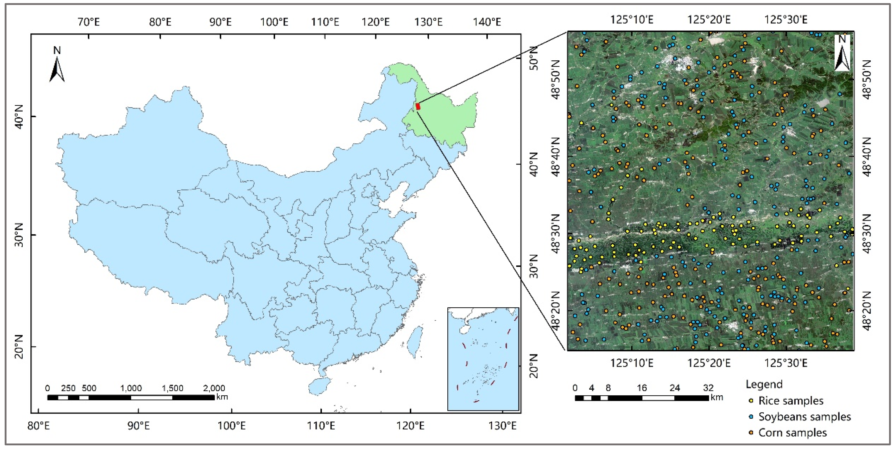
The Songnen Plain is one of the world’s three major black soil areas and is an important commercial grain production base in China. Grain production is related to the national economy’s stability and food security. Our experimental area is located in the western part of the Songnen Plain (125°02′E–127°64′E, 48°24′N–48°94′N) (Figure 1), which has a temperate continental monsoon climate with an average altitude of about 220 m and is suitable for mechanized cultivation of agriculture. The multi-year average temperature ranges from 0 °C to 5 °C, the accumulated temperature ranges from 1800 °C to 2800 °C, and the precipitation ranges from 400 mm to 700 mm. the precipitation is mainly concentrated in the summer months (May–October). Its climatic conditions are favorable for the growth of crops. This region’s main high-quality food crops are corn, soybeans, and rice, which occupy more than 96% of the total area of the study area, and their cropping systems are all harvested one year. Based on the previous phenological period [31], we found that the three crops were basically sown from late April to early May and gradually entered the harvest period from September to October. Rice differs more significantly from other crops during the flooding and transplanting periods. Corn and soybeans have similar phenological periods in the early stages, but there are some differences in the phenological period after entering July, which can be distinguished according to these phenological differences. Their phenological periods are shown in

Table 1. Phenological periods of main crops in the studied region.

Month	Apri		May			June			July			August			September			October
Ten Days	2	3	1	2	3	1	2	3	1	2	3	1	2	3	1	2	3	1
Rice	Sowing	Emergence/Flooding		Transplanting		Reviving		Tillering		Booting		Heading		Milky/Mature		Harvest
Corn		Sowing		Emergence			Three leaves	Seven leaves		Jointing		Heading		Milky/Mature		Harvest
Soybeans		Sowing		Emergence			Three leaves	Bloom		Pod			Mature			Harvest

.

2.2. Data Sources

2.2.1. Satellite Images

The Sentinel-2 mission has two twin satellites, Sentinel-2A and Sentinel-2B, and each identical satellite is equipped with a multispectral sensor, that covers 13 spectral bands and has a swath width of 290 km. Furthermore, this mission monitors the Earth with a resolution of up to 10 m and a revisit time of 5 d after a dual-satellite network. Compared with other multispectral satellite data, the Sentinel-2 satellite has more time and spatial resolution advantages. It can provide more image data resources for the early identification of crops. Spectral characteristics are the essential characteristics of crop recognition and monitoring. This study used ten common features of original spectral bands, including three visible bands, three red-edge bands, one near-infrared band, and two short-wave infrared waves. The Sentinel data resources we used are obtained through the Google Earth Engine (GEE) cloud platform. The platform’s dataset is the Sentinel-2 L2A product, which ESA has pre-processed for radiometric calibration, atmospheric correction, and automatic resampling of the bands to uniform resolution. Hence, the data reflect the reflectance information of the surface. We did the imagery processing to clip each period using the common area SHP to produce an image dataset with a size of 6850 × 7767 pixels. GEE platform not only enables users to easily access and process a large number of geospatial data sets but also reduces the time and energy in the image pre-processing stage, providing a new opportunity for rapid and accurate remote sensing crop information monitoring [32,33,34].

In addition, from the analysis of this study’s date-by-date crop identification results, it was found that the satisfactory accuracy of early crop identification could be reached (≥85%) when used for up to 7 July. Therefore, we collected six available remote sensing images in the early stage, and their information is shown in

Table 2. Image data was used in this study.

Serial Number	Sentinel Image Number	Acquisition Date	Band Name	Cloud Coverage	Width-Height
1	20200428T023549_20200428T024214_T51UXP	28 April 2020	B2, B3, B4, B5, B6, B7, B8, B8A, B11, B12	≤10%	6850 × 7767
2	20200508T023549_20200508T023546_T51UXP	8 May 2020
3	20200513T023551_20200513T023553_T51UXP	13 May 2020
4	20200528T023549_20200528T023954_T51UXP	28 May 2020
5	20200612T023601_20200612T023555_T51UXP	12 June 2020
6	20200707T023549_20200707T023550_T51UXP	7 July 2020

.

2.2.2. Historical Crop Type Mapping

Since the ground data collection work has not been carried out in the early stages of crops, which made a great challenge to early crop identification. Previous studies have shown that historical crop-type mapping contains a large amount of a priori knowledge. There has been a consensus that bulk crops have little difference in crop planting structure over a short period of time [31,32,33]. So, we combined this information with remote sensing images to generate training samples to guide early crop identification in the year to be classified. The historical crop-type mapping was derived from the results of Zhao [35]. It included corn, rice, and soybean, with an overall identification accuracy of 93.12% and a Kappa coefficient of 0.90, which meets the requirements of our study. The process of automatically generating samples based on historical crop-type mapping is: (1) Based on the historical crop-type mapping in 2019, and remote sensing imagery in 2020, candidate images of three crops were obtained by segmentation, respectively. (2) K-means clustering was applied to the candidate image areas to obtain clustering results. The number of clusters was 12. (3) We calculated the area of these sub-clustering results and selected the largest class as the “pure sample” area for each crop type. (4) The pure sample area was raster vectorized, and training sample points for each crop were randomly generated in the top N (the number of training samples of each crop type) sub-vector areas with the largest area. Through the above steps, 823, 815, and 618 samples for corn, soybean, and rice were obtained.

2.2.3. Ground References

The location and crop type of each sample in the study area were recorded with a handheld Global Positioning System (GPS) instrument; the study area’s main object types included corn, rice, soybeans and other land cover types (rivers, water bodies, etc.). Our main target objects are three main crops, so 218 corn samples, 205 soybeans samples, and 156 rice samples were selected to evaluate the classification results of all images for each period. Their spatial distribution is shown in Figure 1.

3. Method

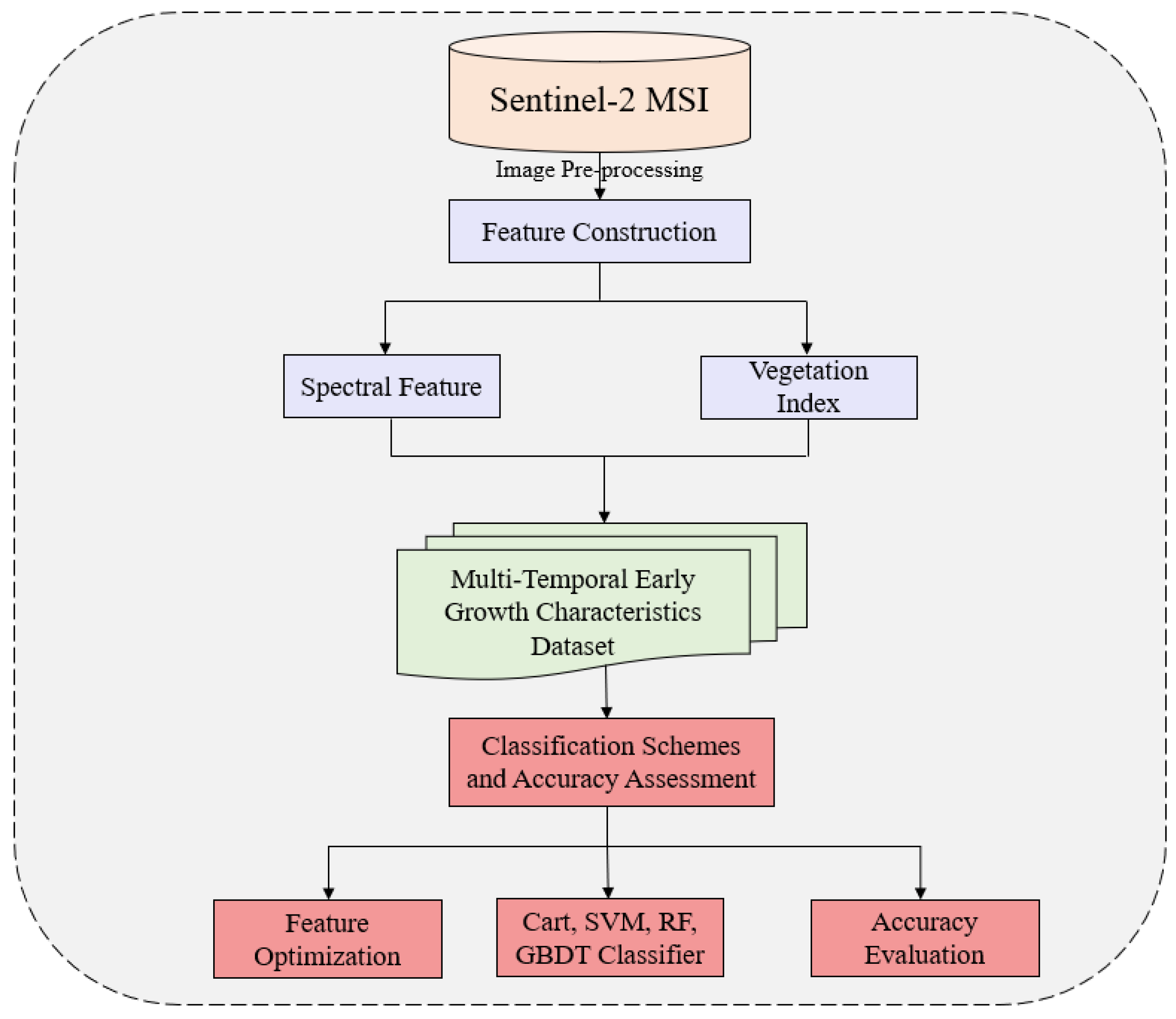
This study mainly focuses on the impact of multi-temporal difference features on early crop identification. It includes three parts. Section 3.1 introduces the spectral and vegetation index features used in single-period remote sensing imagery for the subsequent design of multi-temporal differential features. Section 3.2 presents the combinatorial design of the key change period in the early crop growth period. Based on the crop growth and development characteristics, the image features of different periods were calculated and combined to construct a multi-temporal growth characteristics dataset for early-stage crops. Section 3.3 explores the key periods of change in different crops and their key features. A feature optimization method is used to optimize the most effective features for identifying crops in different periods. Finally, crop recognition is achieved using classification and regression tree (Cart), random forest (RF), gradient boosting decision tree (GBDT), and support vector machine (SVM) modeling. The early crop recognition accuracy is analyzed from different perspectives using various evaluation indicators. The technical route is shown in Figure 2.

3.1. Feature Construction

In terms of the features used, this study excluded B1, B9, and B10 bands with coarse spatial resolution and only used B2, B3, B4, B5, B6, B7, B8, B8A, B11, and B12; these represent 10 original bands and 12 vegetation indices (

Table 3. Vegetation Index used in this study.

Vegetation Index	Formula	Reference
NDVI	$\frac{B_8-B_4}{B_8+B_4}$	[36]
LSWI	$\frac{B_8-B_{11}}{B_8+B_{11}}$	[37]
EVI	$2.5\frac{B_8-B_4}{B_8+6B_4+1-7.5B_2}$	[38]
RESI	$\frac{B_7+B_6-B_5}{B_7+B_6+B_5}$	[39]
RENDVI	$\frac{B_8-B_6}{B_8+B_6}$	[40]
NDRE1	$\frac{B_6-B_5}{B_6+B_5}$	[41]
NDRE2	$\frac{B_7-B_5}{B_7+B_5}$	[42]
NDRE3	$\frac{B_7-B_6}{B_7+B_6}$	[43]
VIgreen	$\frac{B_3-B_4}{B_3+B_4}$	[44]
OSAVI	$1+0.16\frac{B_8-B_4}{B_8+B_4+0.16}$	[45]
NDTI	$\frac{B_{11}-B_{12}}{B_{11}+B_{12}}$	[46]
SR	$\frac{B_8}{B_4}$	[47]

). These indices are selected based on early crop growth characteristics and are widely used in crop identification. Mainly included three categories: (1) The red edge index: Red-edge Spectral Index (RESI), Normalized Difference Red-edge1 (NDRE1), Normalized Difference Red-edge2 (NDRE2), Normalized Difference Red-edge3 (NDRE3), Red Edge Normalized Vegetation Index (RENDVI). (2) Low vegetation cover index: NDVI, Optimization Soil Adjusted Vegetation Index (OSAVI), Normalized Difference Tillage Index (NDTI), Simple Ratio Index (SR). (3) High vegetation cover index: Enhanced Vegetation Index (EVI), Green Vegetation Index (VIgreen).

3.2. Quantitative Description of Crop Early Growth Characteristics

This section describes the growth differences of crops in different periods by constructing differential temporal-phase features. The multi-temporal features are superimposed to increase the amount of early-stage crop information. Each crop has a unique phenology [48,49]. As the crop grows, the spectral reflectance of the crop varies at different periods (Figure 3). The trend of corn and soybean is similar, with a faster growth rate in the early stage, a gradual increase in the middle stage, and a rapid increase or decrease in the later stage, but there are differences in the rate of increase or decrease between the two at different stages. Due to its unique characteristics, the spectral properties of rice are more different from those of the previous two, with a gradual increase in the early stage, followed by a gradual decrease and an upward trend in the later stage. The three crops have different growth rates and show different remote sensing information at different periods [50], indicating that crops can be distinguished by different time phase characteristics. Therefore, the multi-temporal and spectral features were considered together to construct an index of the early growth characteristics of crops. Specifically:

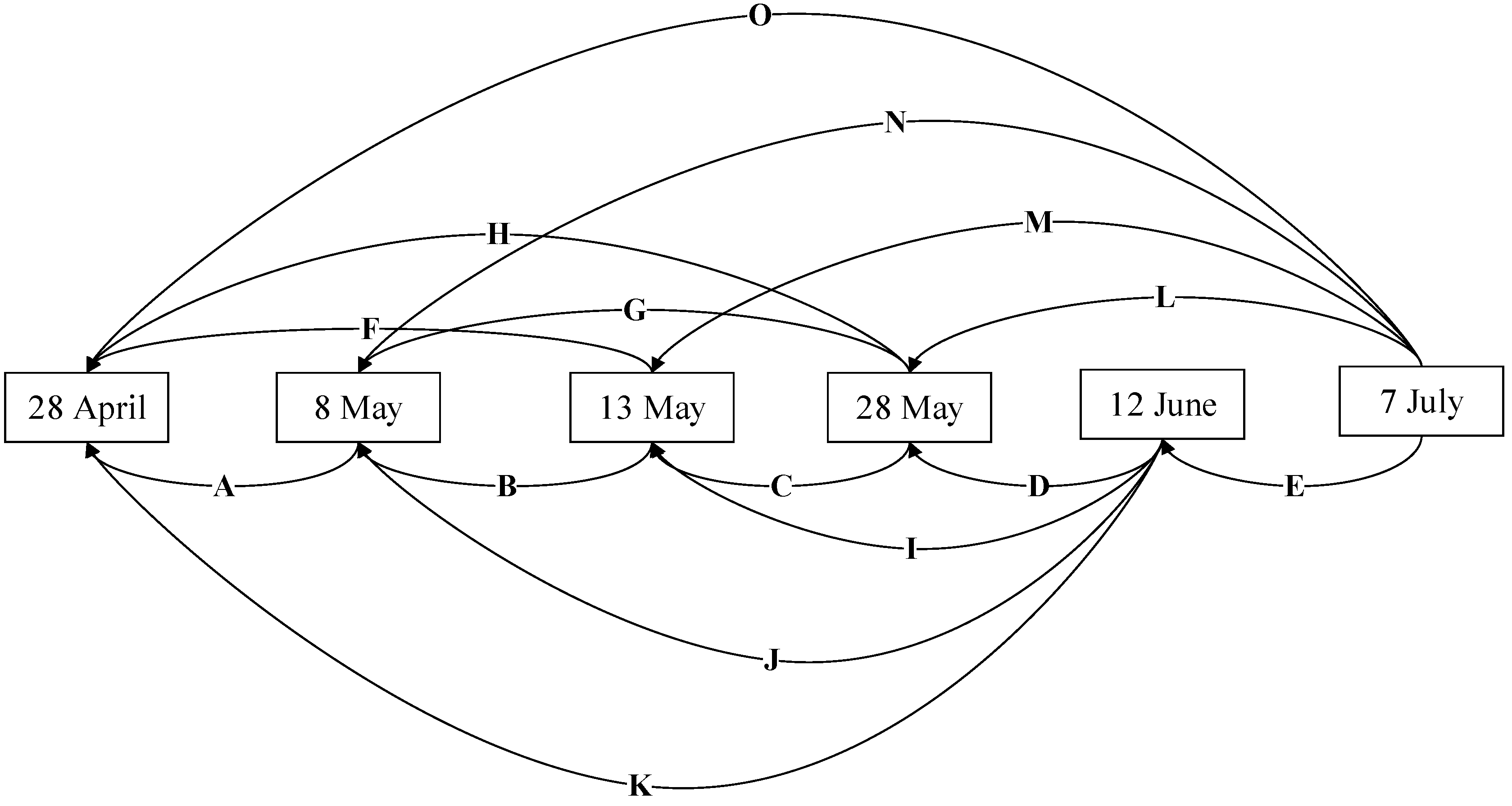
(1) The spectral features of crops are not obvious or easy to distinguish based on a single image of early crop growth [44]. Based on all the remote sensing images collected in the early stages, the different image features were constructed to amplify the performance of crops in different periods. To facilitate understanding, Figure 4 represents the different information in different periods, while

Table 4. Definition of each letter in Figure 4 in 2020 different time phases.

Letter	T2 Date	T1 Date
A	8 May	28 April
B	13 May	8 May
C	28 May	13 May
D	12 June	28 May
E	7 July	12 June
F	13 May	28 April
G	28 May	8 May
H	28 May	28 April
I	12 June	13 May
J	12 June	8 May
K	12 June	28 April
L	7 July	28 May
M	7 July	13 May
N	7 July	8 May
O	7 July	28 April

defines the meaning of each character in the figure represents. The formula for the constructed temporal difference images ($TSDV{I}_{T_1{T}_2}$) is:

$$TSDV{I}_{T_1{T}_2}=V_{T_2}-V_{T_1}$$

(1)

where V comes from the 12 vegetation indices collected in Table 4 and the 10 original bands, $T_2$ represents the current image, $T_1$ represents the prior image, and $T_1$ and $T_2$ were acquired on 28 April, 8 May, 13 May, 28 May; and 12 June, 7 July.

(2) Multi-temporal features can describe the growth characteristics of different crops, which can help improve the accuracy of crop identification [51,52,53]. All possible combinations of images were exhausted based on each period’s different images using the permutation method ($C_n^m$). The band combination was performed according to the m combination type and used as input for uncombined-type image features for that period.

Table 5. Available difference images and total images after band combination for each period in 2020.

Date	Available Difference Time Phase	n	Number of Images after Band Combination (Call)
8 May	A	1	1
13 May	A, B, F	3	7
28 May	A, B, F, C, G, H	6	63
12 June	A, B, F, C, G, H, D, I, J, K	10	1023
7 July	A, B, C, D, E, F, G, H, I, J, K, L, M, N, O	15	32,767

shows the number of available difference images for each period and the total number of images after band combination ($C_{all}$).

Table 6. All possible combination types at each stage and the number of images contained in each type.

Date	1	2	3	4	5	6	7	8	9	10	11	12	13	14	15
7 July	15	105	455	1365	3003	5005	6435	6435	5005	3003	1365	455	105	15	1
12 June	10	45	120	210	252	210	120	45	10	1
28 May	6	15	20	15	6	1
13 May	3	3	1
8 May	1

shows all possible combination types for each period and the number of different images each combination type contains.

$$C_n^m=\frac{A_n^m}{m!}=\frac{m!}{m!\left(n-m\right)!}$$

(2)

$$C_{all}={{\displaystyle \sum }}_{m=1}^n{C}_n^m=2^n-1$$

(3)

where n is the total number of available difference images in each period, m is the combination type, and m ≤ n.

3.3. Classification Schemes and Accuracy Assessment

Although the addition of multi-temporal features can improve crop identification accuracy to a certain extent, not all features play a positive role in recognition [54]. Therefore, the feature optimization method is essentially used to obtain the effective recognition feature set. Finally, different classifiers are modeled to explore the impact of different features on crop recognition accuracy in different periods, as follows:

(1) Feature Optimization

Based on all available images collected in the current period, the different image features in each period are calculated, combined, and then optimized for each combination in each period. Then, the Gini coefficient of RF is used to rank the importance of the optimized feature set. Firstly, Pearson correlation coefficients are used to initially screen out features with correlations above 0.85 and less importance according to the principles that (1) the stronger the correlation, the greater the information redundancy, and (2) the lower the importance of the feature, the weaker its classification ability. Then, RFE is used to perform feature optimization on the remaining features, and the optimal feature collection in each period can be obtained. RFE is used to obtain the optimal feature set by iteratively constructing a model based on the filtered results, removing the features with the lowest scores, and repeating the process until all features have been traversed [55]. A 10-fold cross-validation strategy is used in the selection process to determine the optimal subset of feature variables. Through the above steps, the optimal feature set obtained one differential image on 8 May, seven optimal feature sets on 13 May, 63 optimal feature sets on 28 May 1023 optimal feature sets on 12 June, and 32,767 optimal feature sets on 7 July.

(2) Classification model

In this study, each image’s optimal recognition feature set was used as the input of RF, GBDT, Cart, and SVM classifiers to achieve crop recognition of all images in different periods.

RF classification is composed of multiple decision trees, which have the advantages of strong noise immunity, fast speed, and high accuracy and has been widely used in various classification scenarios [56,57,58]. Its principle is to use bootstrap resampling to extract multiple samples from the original sample, model the decision tree for each bootstrap sample and run it in parallel, and combine the predictions of multiple decision trees to obtain the final prediction according to a voting process. The key parameters are the number of decision tree classifiers (ntree) and the maximum number of features (mtry). The optimal values for ntree are 100, and mtry is 10.

The GBDT classifiers have the advantages of high robustness, high accuracy, and fast speed [59,60]. Its basic principle is to generate a weak Cart regression tree learner, obtain the residuals of the input after training, and then iteratively train the next learner based on the residuals generated by the previous round of learners. During each iteration, each learner aims to minimize the loss function. The final prediction is obtained by accumulating the weak learners’ results. There are some parameters that need to be optimized: learning_rate (the step size when learning), max_features (the number of features to consider when finding the best split) and n_estimators (the number of boosting stages to perform). The search range for learning _rate was set to 0.05 to 0.5 with a search step of 0.05, the search range for max_features was set to 5 to 50 with a search step of 5, and the search range for n_estimators was set to 10 to 300 with a search step of 10. The final parameters for the three were determined to be 0.15, 25, and 150, respectively.

The Cart classifier performs classification tasks based on the generated tree decision rules. It has the advantages of a simple structure and easy interpretation. Therefore, it is widely used in crop identification [61,62]. The algorithm consists of a root node, a series of internal nodes, and leaf nodes; Each internal node represents an attribute judgment, each branch represents a judgment result output, and each leaf node represents a classification result. However, this method also has some drawbacks. Small changes in the training data may affect the tree structure, and a single decision tree is often prone to overfitting and poor generalization. When classifying images, the max_depth is set to 20, the standard is set to “Gini”, the min_samples_leaf is set to 35, and the min_sample_split is set to 10.

The SVM classifier has good generalization ability when the number of samples is limited, and the dimensionality of the feature variables is high [63,64,65]. Therefore, it is widely used to solve classification problems. The principle is to find the optimal hyperplane (decision boundary) to separate the various input training samples (support vectors) from each class. The setting of the kernel type, gamma coefficient, and penalty parameter C in this classifier significantly affects the model performance. The types of kernel functions include “RBF”, “linear”, “sigmoid”, and “poly”. The search values for gamma coefficients include 0.1, 0.2, 0.5, 0.75, and 1, and the search values for C include 1, 2, 4, 8, and 10. The final three were RBF, 0.5, and 4.

(3) Accuracy Assessment

To quantitatively assess the accuracy of the above four classifiers in identifying crops in different periods, the image classification results based on the confusion matrix established from the field validation data were evaluated. The overall accuracy (OA), kappa coefficient, producer accuracy (PA), user accuracy (UA), and F₁-score were selected to reflect the classification accuracy of the images from different aspects [66]. The formula for $F_1$-score is:

$$F_1=2\times \frac{PA\ast UA}{PA+UA}$$

(4)

4. Results

4.1. Trend Analysis of Crop Identification Overall Accuracy and Kappa Coefficient

In this study, the Cart decision tree, GBDT, RF and SVM classifiers were applied to remote sensing recognition of crops in each period. This included 1 recognition result on 8 May, 7 recognition results on 13 May, 63 recognition results on 28 May, 1023 recognition results on 12 June, and 32,767 recognition results on 7 July. The OA and kappa coefficients were used to evaluate the overall crop recognition performance of each classifier in each period. The overall accuracy and kappa coefficient trends in different periods were analyzed as follows.

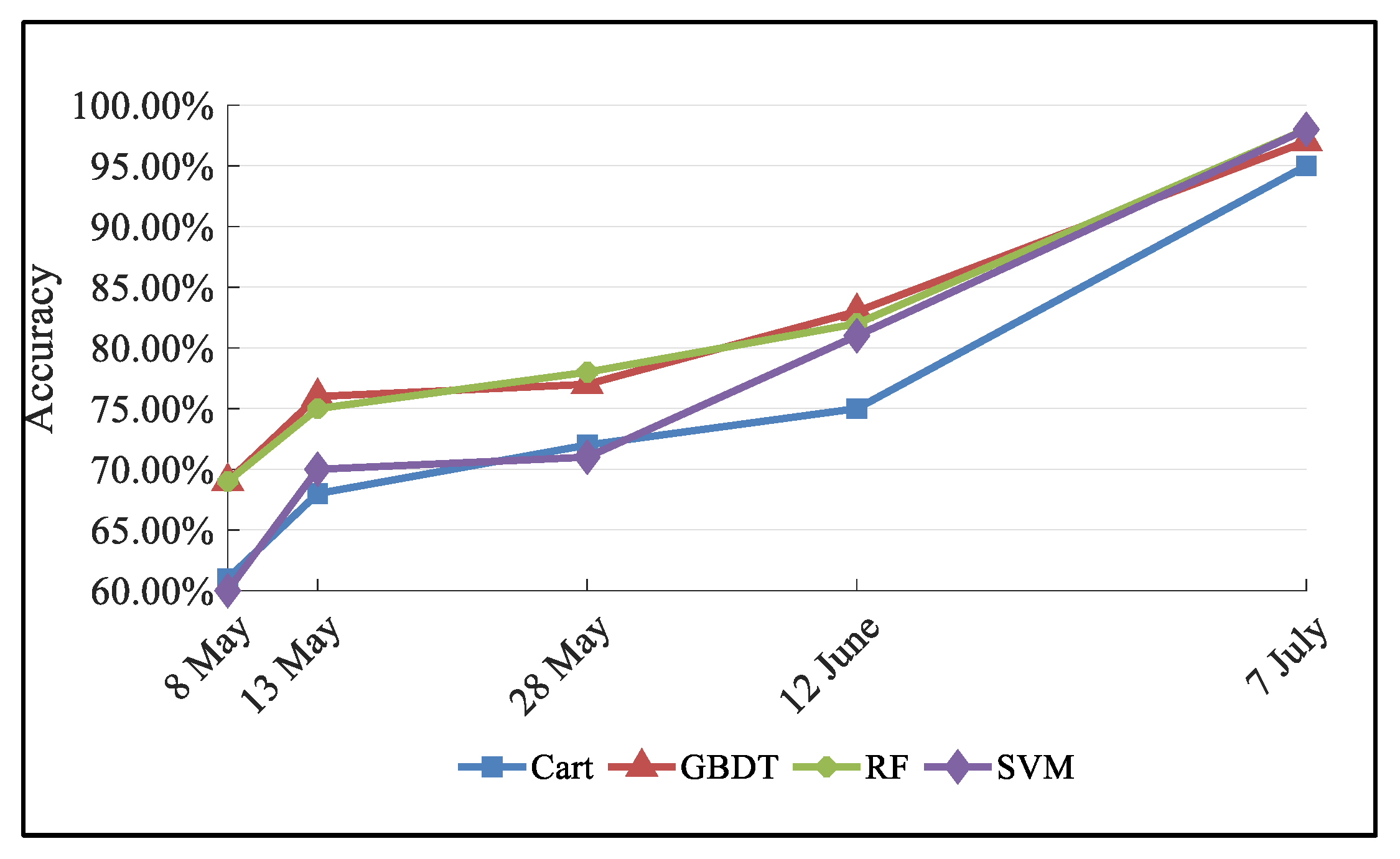
Figure 5 shows the maximum overall recognition accuracy of the four classifiers in different periods. It can be seen that the most significant increase occurred from 12 June to 7 July, when the recognition accuracy increased from 75% to 97%, followed by 8 May to 13 May (60% to 74%). From 13 May to 28 May and 28 May to 12 June, the recognition accuracy changes were relatively low, with ranges of 67–77% and 71–81%, respectively. The OA of the four classifiers tended to increase as more feature information was added over time. The GBDT and RF performed better than the SVM and Cart classifiers throughout the period, with the maximum identification accuracies achieved on 12 June (about 81%) and 7 July (about 97%).

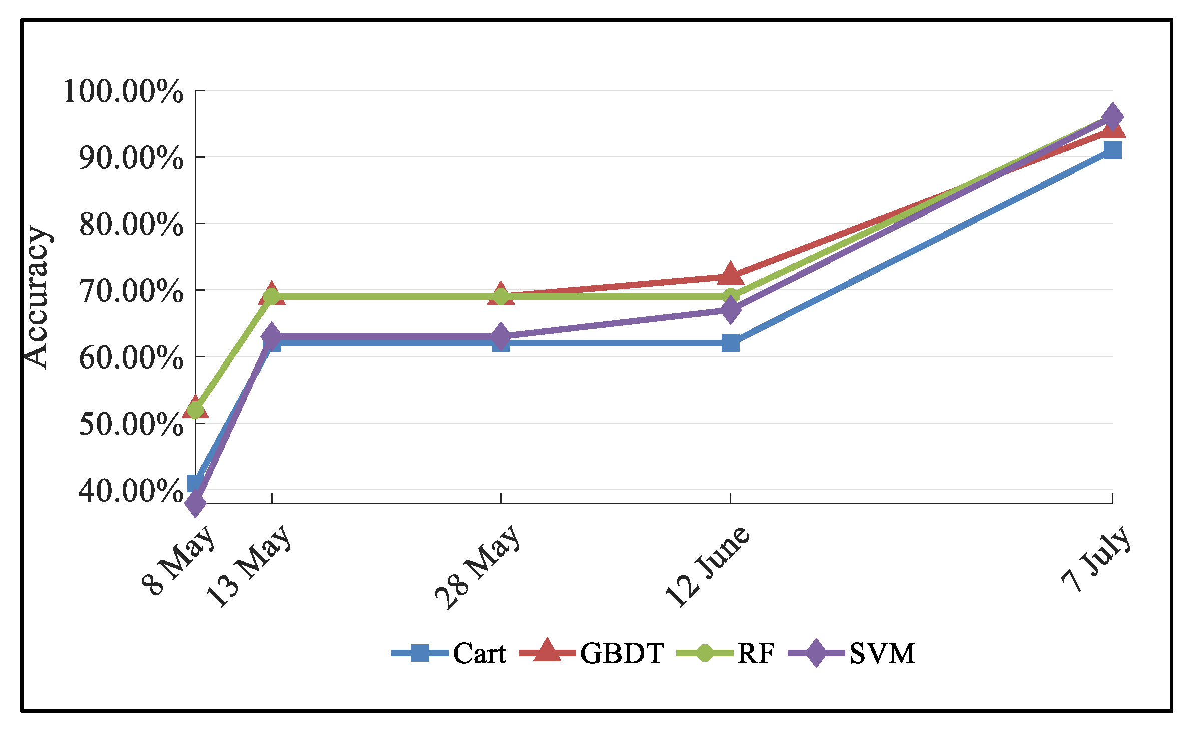
Figure 6 shows the maximum kappa coefficients of the four classifiers in different periods. The upward trend is similar to that of OA during the early stage. The most significant increase occurred from 12 June to 7 July, with a kappa coefficient range of 62–95%, followed by 8 May to 13 May (37–68%). From 13 May to 28 May and 28 May to 12 June, the changes were relatively low (63–68% and 62–71%, respectively). The GBDT and RF performed better than the SVM and Cart classifiers throughout the period, with the kappa coefficients peaking at around 71% on 12 June and about 95% on 7 July.

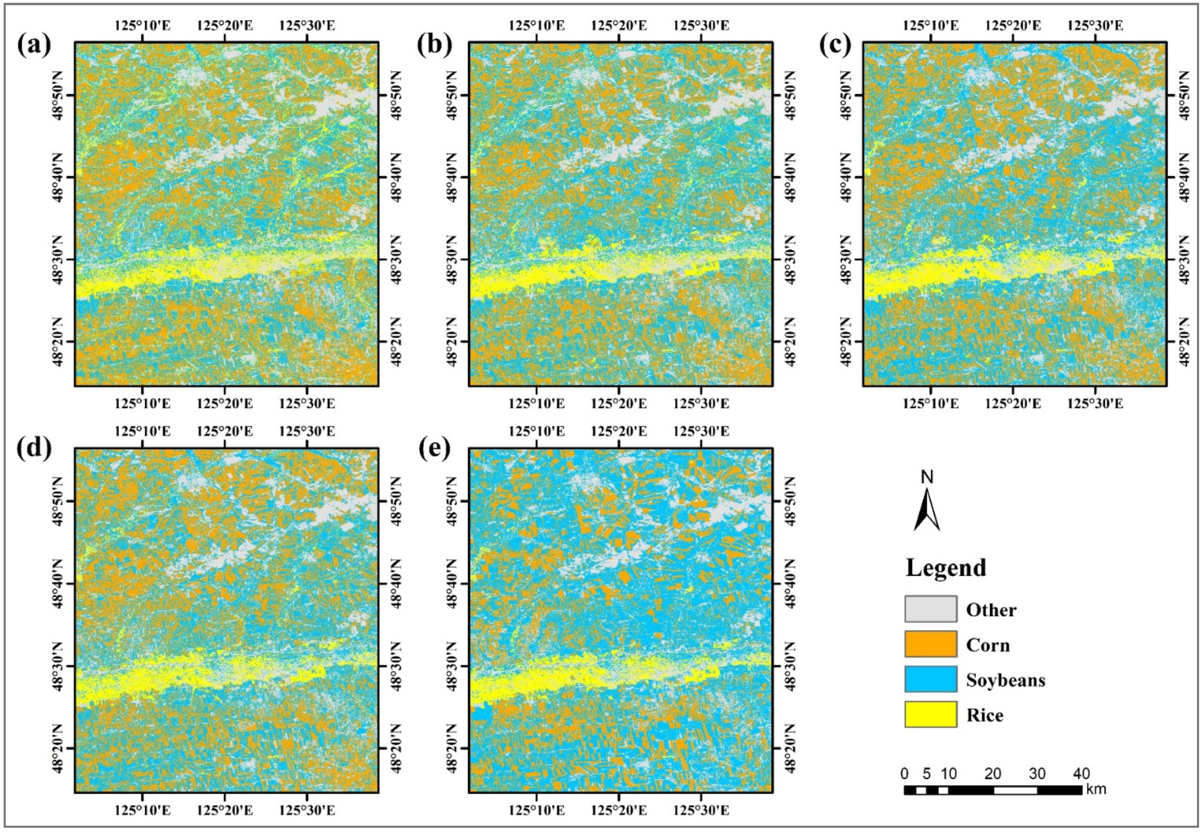
Overall, the identification performance of GBDT and RF was better than those of other classifiers in the early stage, and Figure 7 shows the best recognition results for each period. The performance of SVM was comparable to that of Cart in the early stage, while the recognition ability gradually increased in the later stage, with Cart being worse than the other classifiers.

4.2. Analysis of Trends in Producer Accuracy and User Accuracy

In this study, the PA and UA were used to evaluate the recognition of each crop. The time at which the PA and UA reached above 85% was considered the earliest that each crop was identifiable. The PA and UA recognition analysis for each crop is as follows.

(1) Analysis of trends in producer accuracy and user accuracy for rice identification

Table 7. Maximum PA and UA of rice in 2020 different periods.

Date	Cart		GBDT		RF		SVM
	PA	UA	PA	UA	PA	UA	PA	UA
8 May	77.1%	69.7%	87.9%	80.1%	86.4%	80.2%	86.3%	79.2%
13 May	90%	91.9%	93.6%	95.6%	95.9%	97.7%	91.3%	92.4%

shows the maximum PA and UA achieved by each classifier at different periods for rice identification. The maximum PA was achieved on 8 May (87.9%), and the corresponding UA (80.1%) was lower, so the rice could not be effectively monitored at that time. The RF classifier performed best on 13 May, with its PA and UA being about 95%, followed by the GBDT (about 93%). In contrast, the Cart and SVM did not perform as well as the first two, but both could identify rice effectively, with PA and UA above 90%.

(2) Analysis of trends in producer accuracy and user accuracy for corn identification

Table 8. Maximum PA and UA of corn in 2020 different periods.

Date	Cart		GBDT		RF		SVM
	PA	UA	PA	UA	PA	UA	PA	UA
8 May	57.5%	58.1%	69.5%	64.9%	69%	64.8%	57.5%	62.8%
13 May	64.5%	63.2%	71.5%	71.9%	71%	69.5%	87%	68.8%
28 May	72.5%	69.4%	77.5%	74.9%	78%	75.7%	73.2%	72.7%
12 June	78%	73.8%	83%	81.2%	83%	81.2%	79.5%	80.9%
7 July	98%	97%	98%	98.4%	98%	98.5%	98.5%	97.3%

shows the maximum PA and UA that each classifier could achieve at different times for corn identification. It can be seen that both PA and UA increase with time. In particular, the maximum PA and UA achieved on 12 June was about 81% using GBDT and RF. Corn was able to be identified earliest in the period to 7 July using any of the four classifiers. Their performance was comparable, with the maximum PA and UA both being above 97%.

(3) Analysis of trends in producer accuracy and user accuracy for soybeans identification

Table 9. Maximum PA and UA of soybeans in 2020 different periods.

Date	Cart		GBDT		RF		SVM
	PA	UA	PA	UA	PA	UA	PA	UA
8 May	53%	56.7%	61.5%	64.7%	60%	63.5%	77%	51.2%
13 May	59.5	61.1%	70.5%	69.6%	67.5%	67.2%	77%	58.8%
28 May	70%	69.6%	75.5%	75.5%	77%	75.6%	77%	71.1%
12 June	76%	74.5%	82%	81.6%	82%	81.4%	85%	76.9%
7 July	96.5%	96.9%	99%	97.9%	98.5%	97.9%	94%	95.7%

shows the maximum PA and UA achieved by each classifier for soybeans at different times. As with soybeans identification, the PA and UA of soybean identification also increased over time. The maximum PA and UA on 12 June was also around 81%. On 7 July, all four classifiers could effectively identify soybeans, with GBDT and RF having maximum PA and UA of 97%. The SVM and Cart are somewhat lower at 96% and 94%, respectively.

4.3. Different Remote Sensing Indices Temporal Contribution and Variation Characteristics

Crops have unique growth and seasonal phase-change characteristics. Multi-temporal spectral characteristics can provide effective crop identification information and reveal their changes over time [67]. Usually, the changes in these characteristics are stable and can be used to distinguish between crops over a period of time. This study calculated the importance of all multi-temporal difference features for each period to reflect the relative importance of the features in different periods.

Table A1. Top-10 optimal rice feature sets for different combination types on 8 May 2020.

Combination Type	Letters	F1 Accuracy	Optimum Features
1	A	83.8%	A_NDTI	A_LSWI	A_B11	A_SR	A_B2	A_RENDVI	A_B5	A_NDRE2	A_OSAVI

,

Table A2. Top-10 optimal rice feature sets for different combination types on 13 May 2020.

Combination Type	Letters	F1 Accuracy	Optimum Features
1	F	91.4%	F_NDTI	F_OSAVI	F_LSWI	F_NDVI	F_B8	F_B11	F_NDRE2	F_SR	F_RENDVI	F_B12
2	BF	94.6%	F_NDTI	F_B12	B_B12	B_LSWI	F_B11	F_LSWI	B_RESI	F_NDVI	F_SR	F_B6
3	ABF	92.3%	B_LSWI	F_SR	B_NDTI	A_B11	F_NDTI	F_OSAVI	A_SR	B_SR	F_LSWI	F_B11

,

Table A3. Top-10 optimal corn feature sets for different combination types on 8 May 2020.

Combination Type	Letters	F1 Accuracy	Optimum Features
1	A	67.1%	A_NDTI	A_LSWI	A_B11	A_SR	A_B2	A_RENDVI	A_B5	A_NDRE2	A_OSAVI

,

Table A4. Top-10 optimal corn feature sets for different combination types on 13 May 2020.

Combination Type	Letters	F1 Accuracy	Optimum Features
1	F	69.8%	F_NDTI	F_OSAVI	F_LSWI	F_NDVI	F_B8	F_B11	F_NDRE2	F_SR	F_RENDVI	F_B12
2	AB	71.7%	B_LSWI	A_NDTI	A_B11	B_NDTI	B_OSAVI	A_NDVI	B_SR	A_LSWI	B_B11	A_OSAVI
3	ABF	69.2%	B_LSWI	F_SR	B_NDTI	A_B11	F_NDTI	F_OSAVI	A_SR	B_SR	F_LSWI	F_B11

,

Table A5. Top-10 optimal corn feature sets for different combination types on 28 May 2020.

Combination Type	Letters	F1 Accuracy	Optimum Features
1	H	70.9%	B_SR	H_B12	H_LSWI	H_NDRE1	H_B11	H_B2	H_OSAVI	H_NDRE2	H_NDTI	H_NDVI
2	FG	75.1%	F_SR	F_LSWI	G_LSWI	G_B4	G_NDTI	F_NDTI	G_SR	F_B12	G_B11	F_B11
3	AFG	76.8%	A_LSWI	F_SR	G_B11	G_LSWI	A_SR	A_RENDVI	G_B12	G_RENDVI	F_B11	F_B12
4	ABCF	75.9%	C_LSWI	C_B11	F_LSWI	F_SR	C_B12	F_NDTI	B_RESI	B_SR	C_B8	C_NDTI
5	ABCGH	76.2%	C_SR	G_LSWI	B_LSWI	H_SR	H_B11	G_B11	C_NDTI	A_NDVI	H_NDTI	C_LSWI
6	ABCFGH	73.4%	C_SR	C_NDTI	H_B11	C_LSWI	C_B11	H_NDTI	G_LSWI	A_NDTI	F_OSAVI	F_LSWI

,

Table A6. Top-10 optimal corn feature sets for different combination types on 12 June 2020.

Combination Type	Letters	F1 Accuracy	Optimum Features
1	K	72%	K_B11	K_NDTI	K_LSWI	K_OSAVI	K_EVI	K_B3	K_B5	K_B12
2	DK	78.2%	D_SR	D_NDTI	K_NDTI	K_NDVI	D_LSWI	K_B11	K_OSAVI	D_NDVI	K_LSWI	K_B8A
3	CHJ	79.4%	J_LSWI	H_B11	H_NDTI	H_B12	A_SR	J_RENDVI	C_NDTI	C_OSAVI	H_LSWI	J_B5
4	BDFJ	80.2%	J_SR	J_NDVI	F_B12	F_LSWI	D_OSAVI	F_B3	F_OSAVI	J_NDRE3	F_B11	J_RESI
5	CDHIJ	82%	J_LSWI	H_SR	I_B11	C_NDTI	D_NDVI	J_EVI	H_LSWI	D_LSWI	D_B11	H_B12
6	BCDFGJ	80.8%	D_SR	J_NDTI	F_B11	G_LSWI	G_NDTI	J_LSWI	G_SR	F_NDRE1	C_LSWI	F_NDVI
7	ABDFHJK	80.3%	J_LSWI	H_LSWI	J_SR	J_RENDVI	J_NDRE3	D_NDVI	J_B11	B_NDVI	F_LSWI	K_SR
8	ABCDGHIJ	80.8%	G_NDTI	J_LSWI	H_B12	G_SR	H_NDRE1	A_NDTI	I_SR	C_NDTI	J_B6	D_EVI
9	ABCDFGHJK	80%	J_LSWI	F_B11	D_LSWI	J_NDTI	C_LSWI	B_LSWI	H_B11	F_LSWI	G_B11	C_NDTI
10	ABCDFGHIJK	78.7%	H_LSWI	I_NDTI	D_SR	F_B11	J_LSWI	G_LSWI	G_SR	H_NDTI	H_B11	D_NDRE3

,

Table A7. Top-10 optimal corn feature sets for different combination types on 7 July 2020.

Combination Type	Letters	F1 Accuracy	Optimum Features
1	E	94%	E_B11	E_NDRE3	E_NDRE2	E_LSWI	E_B6	E_B4	E_VIgreen	E_B8	E_EVI	E_B5
2	EO	95.9%	E_NDRE3	E_VIgreen	E_B11	E_NDRE2	E_RESI	E_LSWI	O_NDRE1	E_RENDVI	O_NDRE2	O_NDRE3
3	EHI	96.9%	E_NDRE3	E_RESI	E_LSWI	E_EVI	H_NDTI	H_VIgreen	H_B11	E_VIgreen	E_B12	H_NDRE2
4	CEHJ	97%	E_NDRE3	E_B11	E_LSWI	H_B11	E_NDRE2	H_B12	E_RESI	I_NDRE2	E_VIgreen	H_NDRE2
5	EHIMO	97.3%	E_NDRE3	H_B11	E_B11	M_RESI	M_LSWI	H_VIgreen	E_NDRE2	O_EVI	H_B12	M_B11
6	BEFHIM	97.3%	I_LSWI	F_LSWI	I_EVI	E_NDRE2	I_RESI	E_VIgreen	F_B11	B_LSWI	E_RENDVI	H_RESI
7	BCDEHKM	97.3%	E_NDRE3	E_B11	E_LSWI	M_B11	M_NDRE3	H_B11	H_RESI	K_VIgreen	E_RESI	M_LSWI
8	CEFGHIKM	98.2%	E_NDRE3	E_B11	M_NDRE3	M_LSWI	E_LSWI	M_VIgreen	K_B11	G_B11	M_NDRE2	H_RESI
9	ACDEFGHMN	98.2%	E_NDRE3	E_B11	M_RESI	M_NDRE3	H_B11	N_NDRE3	M_LSWI	E_LSWI	E_EVI	A_NDRE2
10	BCDEGHKLMN	97.3%	L_NDRE3	L_B11	E_B11	E_NDRE3	H_B11	E_LSWI	L_LSWI	M_LSWI	M_NDRE3	K_B11
11	BDEFGHIJKLM	96.3%	E_NDRE3	L_B11	L_NDRE3	E_B11	E_LSWI	L_LSWI	M_NDRE3	M_LSWI	K_VIgreen	M_B11
12	ABDEFGHIKLMO	97%	L_B11	L_LSWI	E_B11	E_NDRE3	L_NDRE3	H_B11	E_LSWI	M_LSWI	K_B11	M_NDRE3
13	CDEFGHIJKLMNO	97%	E_B11	M_VIgreen	E_NDRE3	L_LSWI	L_NDRE3	L_RESI	F_EVI	H_VIgreen	K_B11	M_LSWI
14	ABCDEFGHIJKLMO	97.2%	L_NDRE3	M_NDRE3	L_LSWI	L_NDRE2	L_B11	E_NDRE3	L_RESI	E_B11	O_NDRE2	O_RESI
15	ABCDEFGHIJKLMNO	96.4%	L_NDRE3	E_NDRE3	L_B11	L_LSWI	M_NDRE3	E_B11	H_B12	L_NDRE1	E_VIgreen	K_B8A

,

Table A8. Top-10 optimal soybeans feature sets for different combination types on 8 May 2020.

Combination Type	Letters	F1 Accuracy	Optimum Features
1	A	63%	A_NDTI	A_LSWI	A_B11	A_SR	A_B2	A_RENDVI	A_B5	A_NDRE2	A_OSAVI

,

Table A9. Top-10 optimal soybeans feature sets for different combination types on 13 May 2020.

Combination Type	Letters	F1 Accuracy	Optimum Features
1	F	67.5%	F_NDTI	F_OSAVI	F_LSWI	F_NDVI	F_B8	F_B11	F_NDRE2	F_SR	F_RENDVI	F_B12
2	AB	68.5%	B_LSWI	A_NDTI	A_B11	B_NDTI	B_OSAVI	A_NDVI	B_SR	A_LSWI	B_B11	A_OSAVI
3	ABF	70%	B_LSWI	F_SR	B_NDTI	A_B11	F_NDTI	F_OSAVI	A_SR	B_SR	F_LSWI	F_B11

,

Table A10. Top-10 optimal soybeans feature sets for different combination types on 28 May 2020.

Combination Type	Letters	F1 Accuracy	Optimum Features
1	H	69.5%	B_SR	H_B12	H_LSWI	H_NDRE1	H_B11	H_B2	H_OSAVI	H_NDRE2	H_NDTI	H_NDVI
2	AG	74.1%	G_NDRE2	G_LSWI	G_NDTI	G_RENDVI	A_B11	A_B12	A_LSWI	A_NDTI	A_SR	G_B11
3	AFG	76.2%	A_LSWI	F_SR	G_B8	G_LSWI	A_SR	A_RENDVI	G_B12	G_RENDVI	F_B11	F_B12
4	ABCF	74.7%	C_LSWI	C_B11	F_LSWI	F_SR	C_B12	F_NDTI	B_RESI	B_SR	C_B8	C_NDTI
5	ABCGH	74.7%	C_SR	G_LSWI	B_LSWI	H_SR	H_B11	G_B11	C_NDTI	A_NDVI	H_NDTI	C_LSWI
6	ABCFGH	73.3%	C_SR	C_NDTI	H_B11	C_LSWI	C_B11	H_NDTI	G_LSWI	A_NDTI	F_OSAVI	F_LSWI

,

Table A11. Top-10 optimal soybeans feature sets for different combination types on 12 June 2020.

Combination Type	Letters	F1 Accuracy	Optimum Features
1	K	72.3%	K_B11	K_NDTI	K_LSWI	K_OSAVI	K_EVI	K_B3	K_B5	K_B12
2	HK	77.5%	K_OSAVI	K_B11	H_NDTI	K_B5	K_LSWI	K_NDRE1	K_VIgreen	H_NDRE1	K_B3	H_SR
3	CFI	79.4%	I_LSWI	C_LSWI	I_RENDVI	F_B11	F_NDTI	C_NDTI	C_B3	F_LSWI	I_NDTI	C_B8
4	BFHI	80.1%	I_LSWI	I_B11	B_LSWI	H_NDRE3	F_B11	F_LSWI	H_NDTI	H_B11	F_B12	F_NDVI
5	CDHIJ	81.8%	J_LSWI	H_SR	I_B11	C_NDTI	D_NDVI	J_EVI	H_LSWI	D_LSWI	D_B11	H_B12
6	BCDFGJ	80.2%	D_SR	J_NDTI	F_B11	G_LSWI	G_NDTI	J_LSWI	G_SR	F_NDRE1	C_LSWI	F_NDVI
7	ABDFHJK	80.2%	J_LSWI	H_LSWI	J_SR	J_RENDVI	J_NDRE3	D_NDVI	J_B11	B_NDVI	F_LSWI	K_SR
8	ABCDGHIJ	78.9%	G_NDTI	J_LSWI	H_B12	G_SR	H_NDRE1	A_NDTI	I_SR	C_NDTI	J_B6	D_EVI
9	ABCDFGHJK	79.5%	J_LSWI	F_B11	D_LSWI	J_NDTI	C_LSWI	B_LSWI	H_B11	F_LSWI	G_B11	C_NDTI
10	ABCDFGHIJK	76.8%	H_LSWI	I_NDTI	D_SR	F_B11	J_LSWI	G_LSWI	G_SR	H_NDTI	H_B11	D_NDRE3

and

Table A12. Top-10 optimal soybeans feature sets for different combination types on 7 July 2020.

Combination Type	Letters	F1 Accuracy	Optimum Features
1	N	94.1%	N_LSWI	N_NDRE3	N_EVI	N_NDVI	N_NDRE2	N_VIgreen	N_B12	N_B7	N_RESI	N_SR
2	KN	96.3%	N_NDRE3	K_EVI	K_B12	N_NDRE2	N_LSWI	N_B11	N_EVI	K_B11	K_LSWI	N_VIgreen
3	EHI	97.3%	E_NDRE3	E_RESI	E_LSWI	E_EVI	H_RESI	H_VIgreen	H_B11	E_VIgreen	E_B12	H_NDRE2
4	CEHJ	96.9%	E_NDRE3	E_B11	E_LSWI	H_B11	E_NDRE2	H_B12	E_RESI	I_NDRE2	E_VIgreen	H_NDRE2
5	EHIJN	97.3%	E_NDRE3	N_VIgreen	H_B11	E_B12	E_VIgreen	N_LSWI	H_B12	E_LSWI	H_RESI	E_NDRE2
6	BEFHIM	98.5%	I_LSWI	F_LSWI	I_EVI	E_NDRE2	I_RESI	E_VIgreen	F_B11	B_LSWI	E_RENDVI	H_RESI
7	DEFHJKM	97.3%	E_NDRE3	E_B11	M_B12	E_LSWI	M_B11	H_B12	M_LSWI	E_RESI	E_EVI	K_RESI
8	CEFGHIKM	98.5%	E_NDRE3	E_B11	M_NDRE3	M_LSWI	E_LSWI	M_VIgreen	K_B11	G_B11	M_NDRE2	H_RESI
9	ACDEFGHMN	97.3%	E_NDRE3	E_B11	M_RESI	M_NDRE3	H_B11	N_NDRE3	M_LSWI	E_LSWI	E_EVI	A_NDRE2
10	ABCDEFGHJM	97.3%	E_B11	E_NDRE3	M_NDRE3	M_B11	H_B11	M_LSWI	E_RESI	D_EVI	G_B11	M_EVI
11	ABCDEFIJKMN	97.3%	E_B11	E_NDRE3	N_NDRE3	E_LSWI	K_VIgreen	K_B11	K_LSWI	N_LSWI	M_NDRE3	M_EVI
12	ABDEFGHIKLMO	97%	L_B11	L_LSWI	E_B11	E_NDRE3	L_NDRE3	H_B11	E_LSWI	M_LSWI	K_B11	M_NDRE3
13	CDEFGHIJKLMNO	96.7%	E_B11	M_VIgreen	E_NDRE3	L_LSWI	L_NDRE3	L_RESI	F_EVI	H_VIgreen	K_B11	M_LSWI
14	ACDEFGHIJKLMNO	97.3%	E_NDRE3	L_VIgreen	L_B11	H_B12	L_LSWI	N_NDRE3	E_B11	M_NDRE3	L_B12	E_VIgreen
15	ABCDEFGHIJKLMNO	96.4%	L_NDRE3	E_NDRE3	L_B11	L_LSWI	M_NDRE3	E_B11	H_B12	L_NDRE1	E_VIgreen	K_B8A

summarizes the top 10 optimal feature sets of each best combination type of three crops in each period. Features with a higher proportion and ranking are better for crop identification [54]. The key spectral and temporal characteristics of the three crops are analyzed as follows.

(1) Early identifying characteristics and temporal changes characteristics of rice

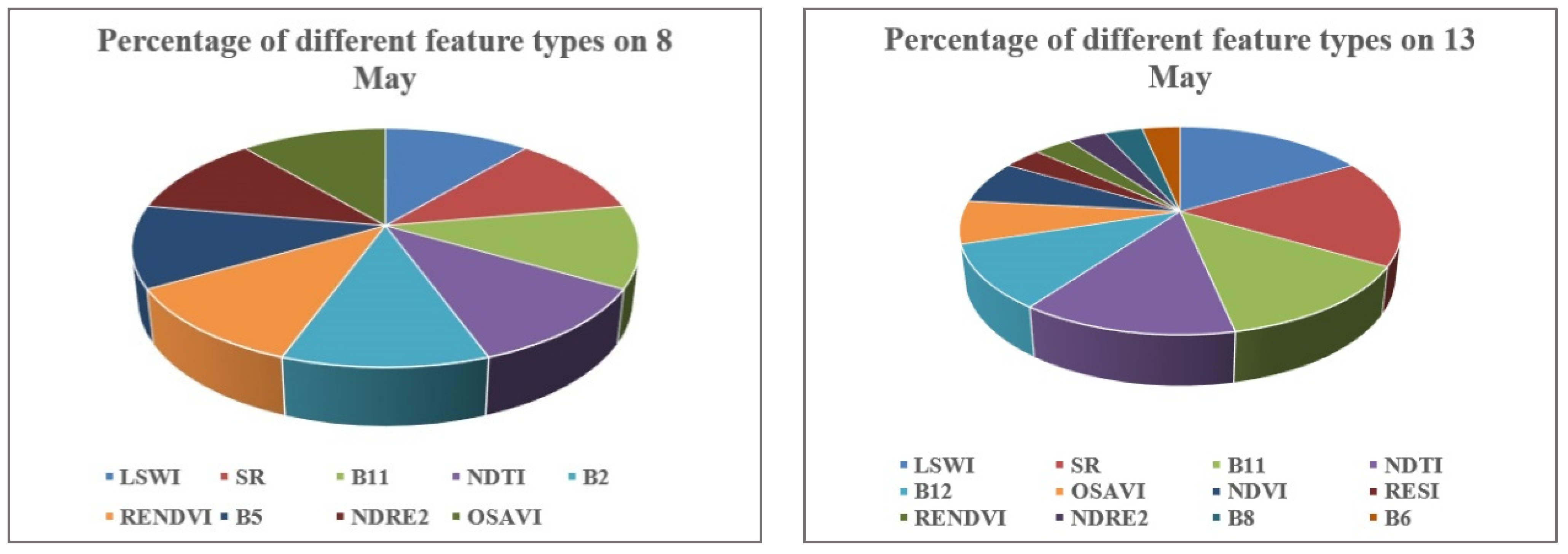
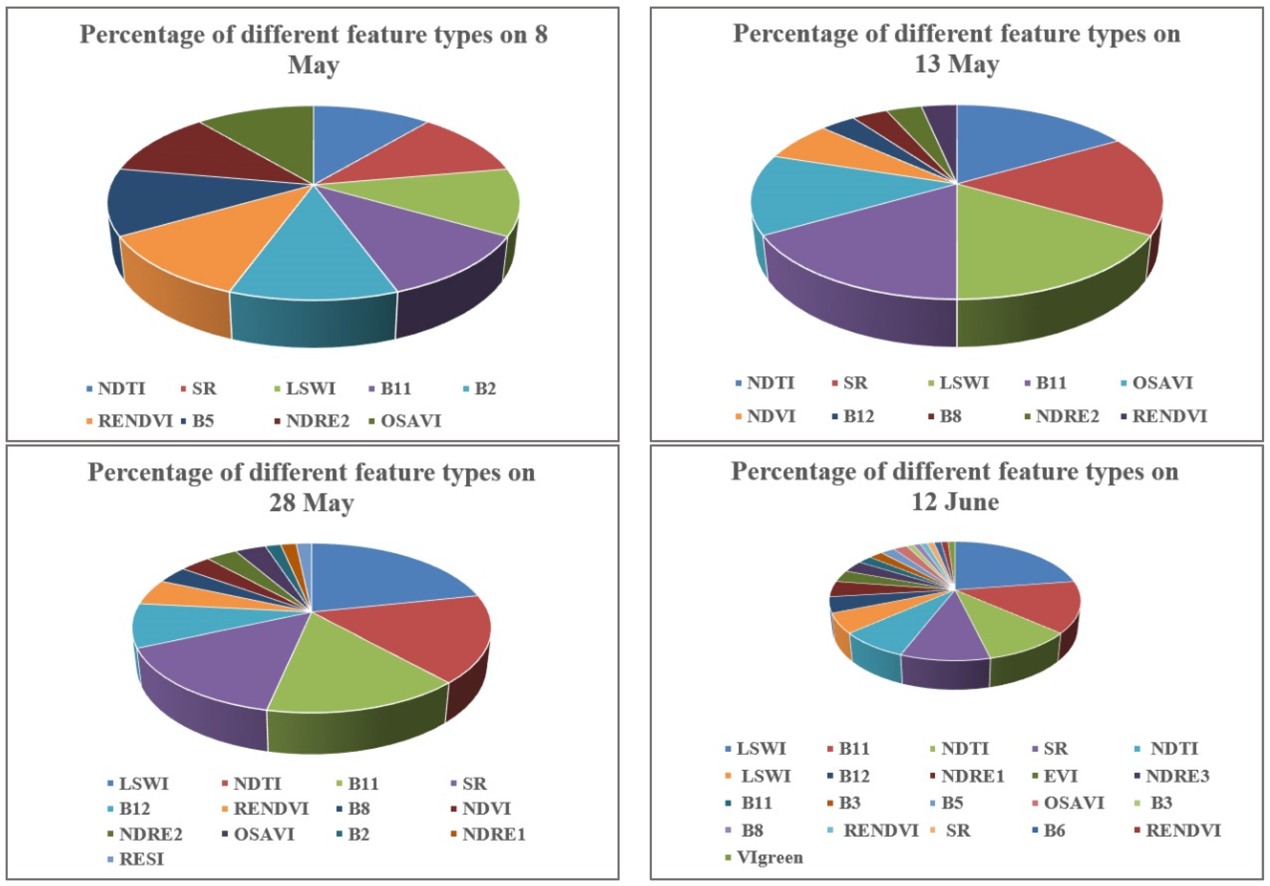
Figure 8 shows the proportions of feature types in the top10 optimal rice feature sets of all best combination types in each period. Rice is a typical paddy crop, which behaves as a mixture of water and paddy in the early stage. The LSWI, SR, B11, and NDTI can effectively reflect the water changes in the canopy and canopy background during the growth and development of rice in this period so that rice crops can be effectively identified.

Table 10. The top-10 optimal feature sets of best rice combination types for each period in 2020.

Date	Best Combination Type	F1 Accuracy	Optimum Features
8 May	A	83.8%	A_NDTI	A_LSWI	A_B11	A_SR	A_B2	A_RENDVI	A_B5	A_NDRE2	A_OSAVI
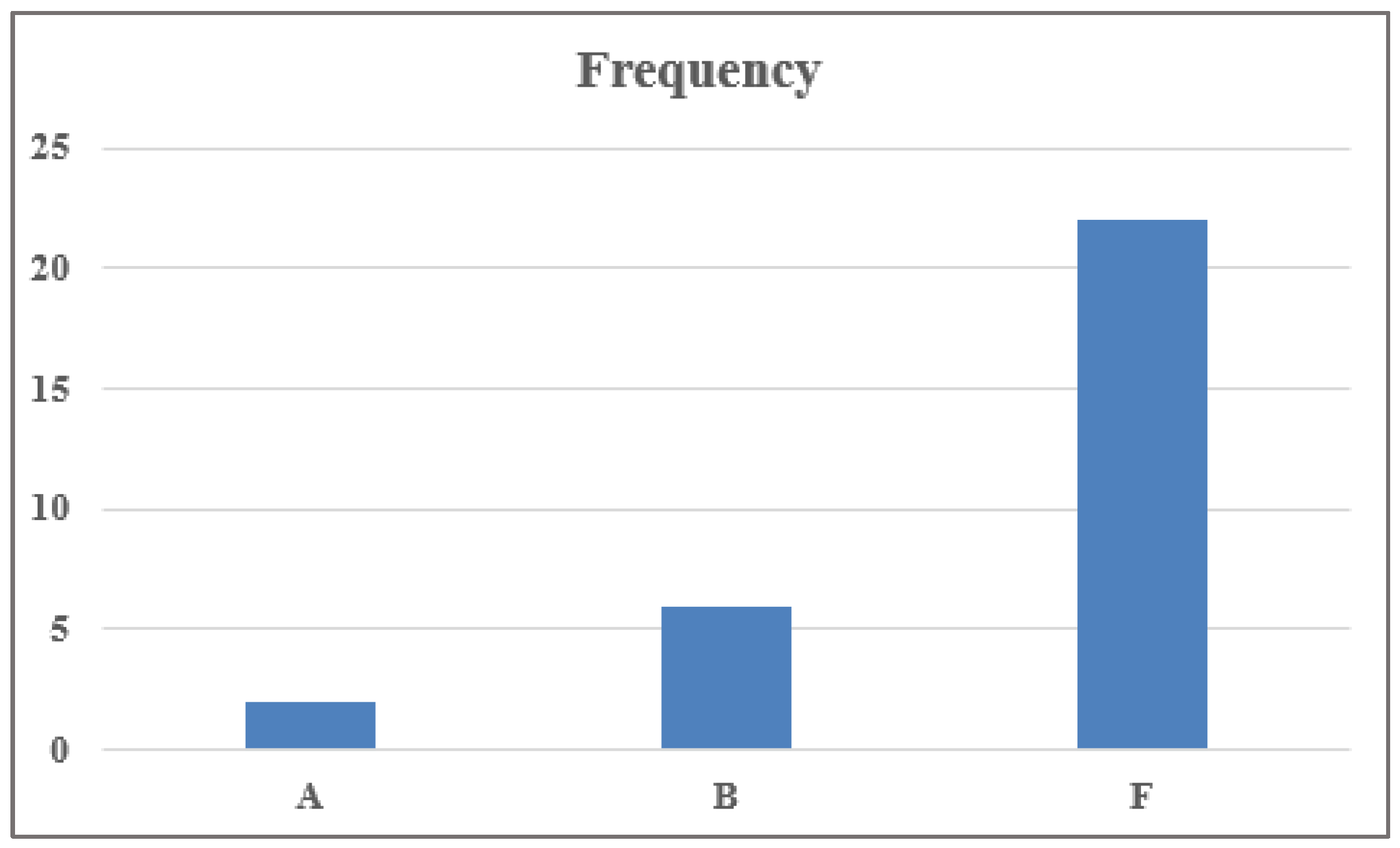
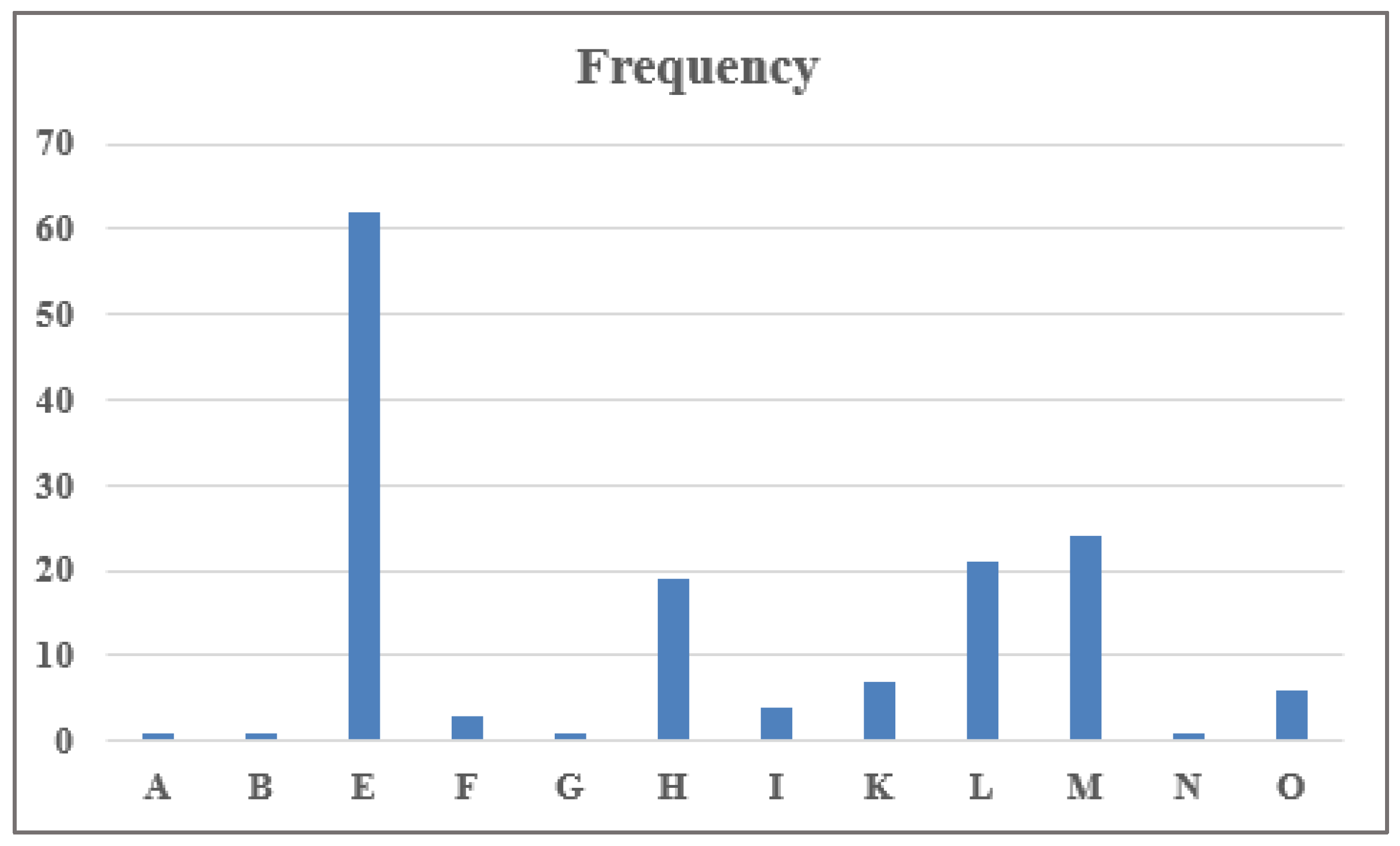
13 May	BF	94.6%	F_NDTI	F_B12	B_B12	B_LSWI	F_B11	F_LSWI	B_RESI	F_NDVI	F_SR	F_B6

shows the top10 optimal feature sets of the best combination types for rice in each period. It can be seen that on 8 May, only one combination of differential temporal phases (A) was able to achieve 81% recognition accuracy. On 13 May, two combinations of BF achieved the maximum classification accuracy (94.6%). In addition, the maximum recognition accuracy of each combination in that period was able to meet the requirement for early recognition of rice (≥91%). Figure 9 shows the frequency of key temporal changes in the top10 feature sets of all the best combination types for rice on 13 May. The frequency of F was significantly greater than those of the other different temporal phases, indicating that the difference in remote sensing information between 13 May and 28 April is key information for early rice crop identification.

(2) Early identifying characteristics and temporal changes characteristics of corn

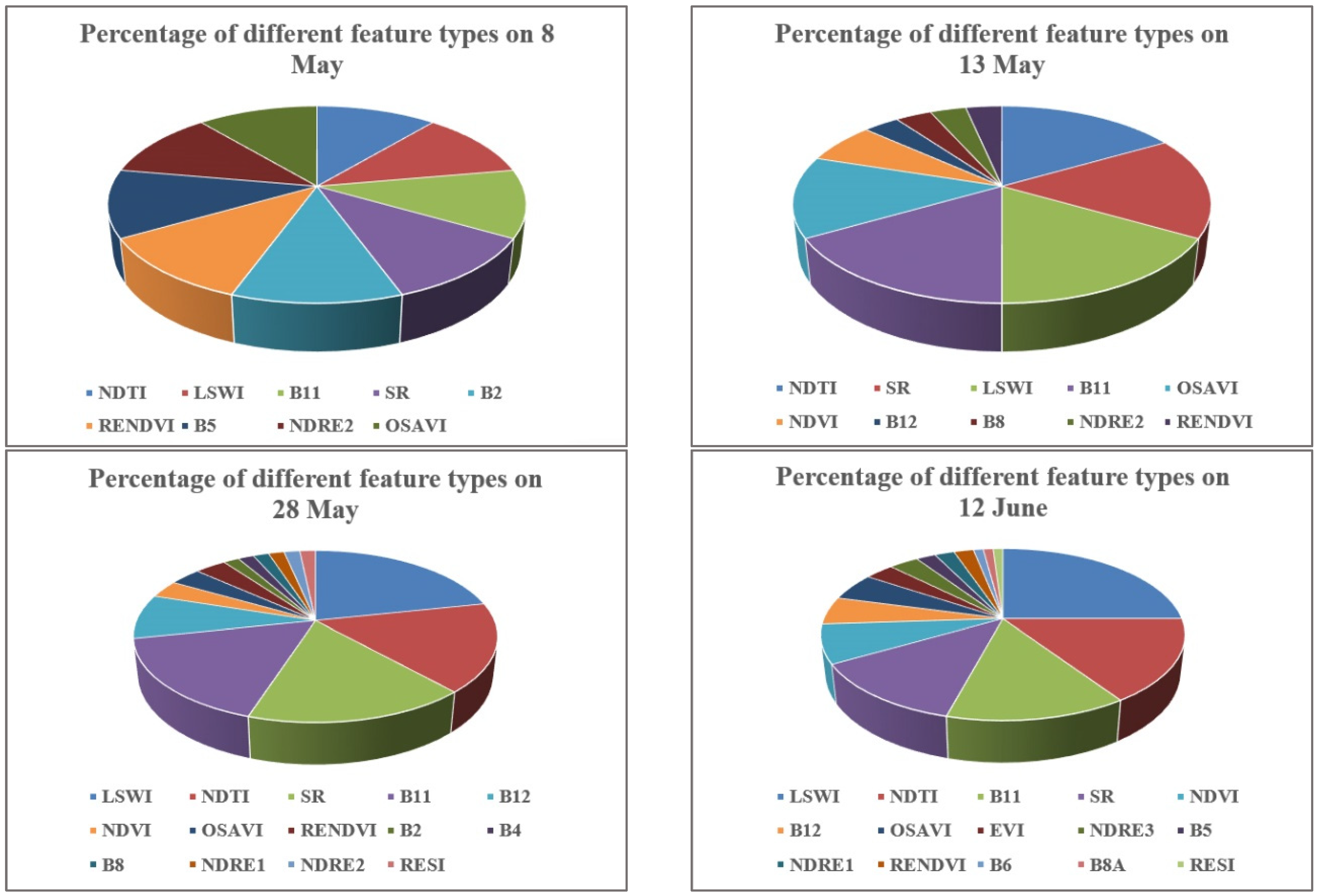
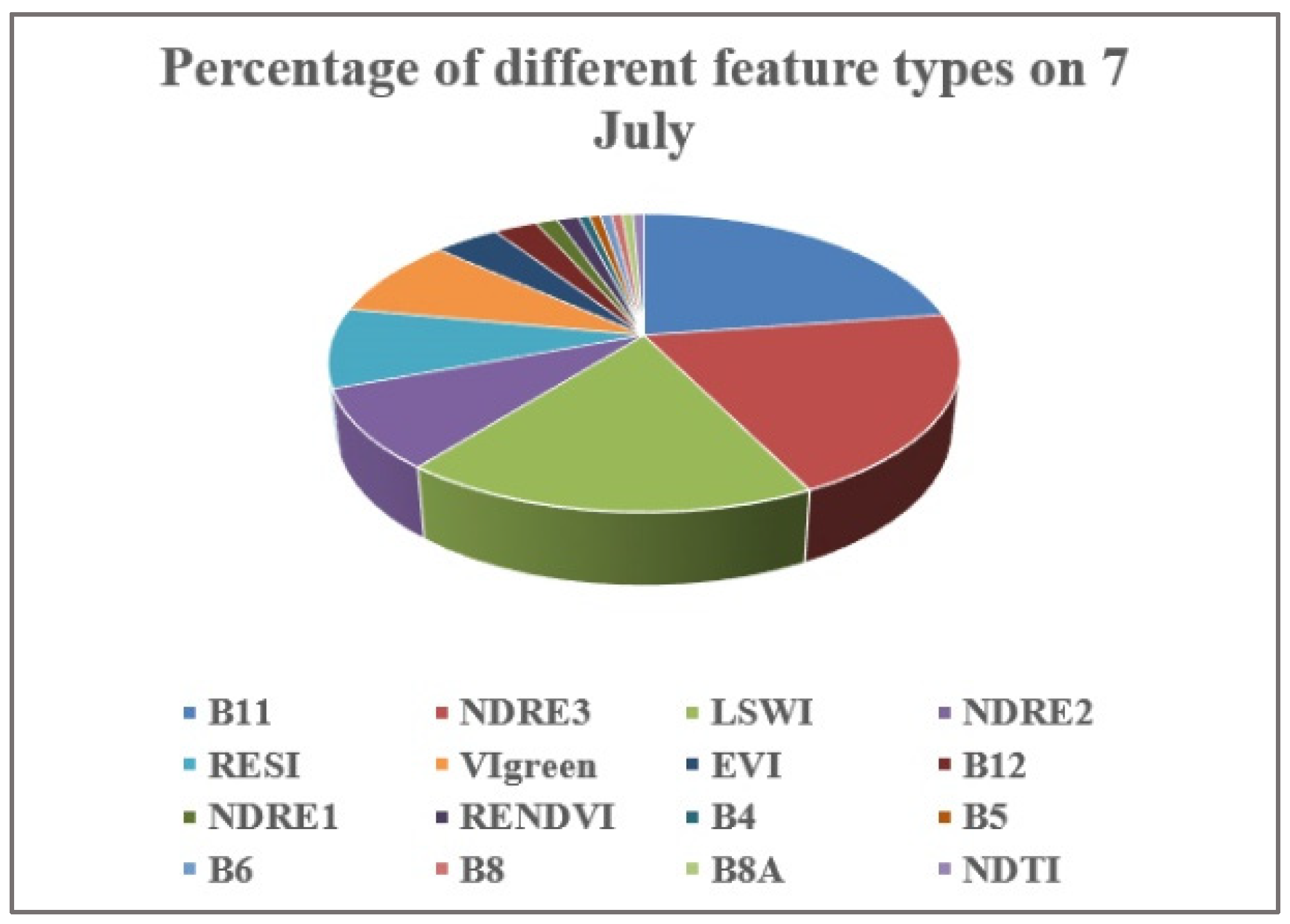
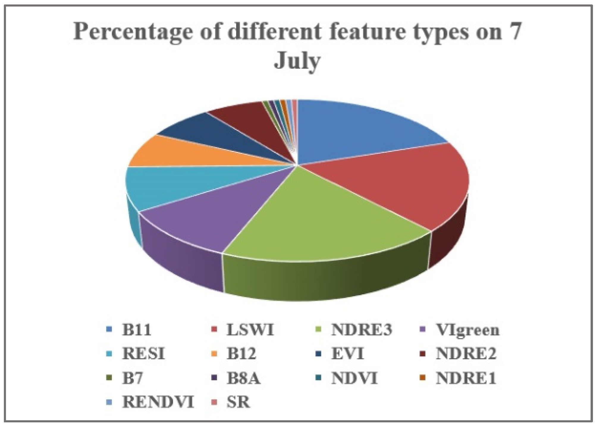
Figure 10 shows the proportion of different feature types in the top-10 optimal corn feature sets of all best combination types at each period. By early June, corn had undergone the sowing and emergence stages, and the images acquired at that time showed low vegetation cover information. The NDTI, SR, LSWI, and B11 accounted for a relatively large proportion during this period. As the crop grows, it gradually enters its peak growth period. In early July, when corn is at the seventh leaf stage, the vegetation cover is greater compared to the previous months. Features such as short-wave infrared bands, some vegetation red-edge bands, and indices of vegetation cover (B11, NDRE3, LSWI, VIgreen, RESI, NERED2) become more prominent and can effectively capture corn growth information.

Table 11. The top-10 optimal feature set of best corn combination types for each period in 2020.

Date	Best Combination Type	F1 Accuracy	Optimum Features
8 May	A	67.1%	A_NDTI	A_LSWI	A_B11	A_SR	A_B2	A_RENDVI	A_B5	A_NDRE2	A_OSAVI
13 May	AB	71.7%	B_LSWI	A_NDTI	A_B11	B_NDTI	B_OSAVI	A_NDVI	B_SR	A_LSWI	B_B11	A_OSAVI
28 May	AFG	76.8%	A_LSWI	F_SR	G_B11	G_LSWI	A_SR	A_RENDVI	G_B12	G_RENDVI	F_B11	F_B12
12 June	CDHIJ	82%	J_LSWI	H_SR	I_B11	C_NDTI	D_NDVI	J_EVI	H_LSWI	D_LSWI	D_B11	H_B12
7 July	CEFGHIKM	98.2%	E_NDRE3	E_B11	M_NDRE3	M_LSWI	E_LSWI	M_VIgreen	K_B11	G_B11	M_NDRE2	H_RESI
	ACDEFGHMN	98.2%	E_NDRE3	E_B11	M_RESI	M_NDRE3	H_B11	N_NDRE3	M_LSWI	E_LSWI	E_EVI	A_NDRE2

shows the top10 optimal feature sets of the best combination types for corn identification in each period. On 8 May, a 67.1% corn recognition accuracy was achieved with index combination A. The maximum recognition accuracy for the period to 13 May (72%) was achieved using the two combinations of AB. The classification achieved the maximum recognition accuracy for the period to 28 May (76.8%) using the three combinations of ABF. On 12 June, the maximum recognition accuracy for the period was achieved using five combinations of CDHIJ (82%). On 7 July, the maximum recognition accuracy for the period (98.2%) was achieved using eight and nine combinations of CEFGHIKM and ACDEFGHMN. In addition, the best combination of 15 combinations for the period achieved satisfactory early identification accuracy for corn (≥94%). Figure 11 shows the frequency of key change temporal in the top-10 feature sets of all the best combination types for corn in this period. E, M, and L appeared to have higher frequencies indicating that the differences between 7 July and 12 June and 13 May and 28 May were obvious enough to identify corn effectively. In addition, the growth difference information on 28 May and 28 April (H) was also obvious.

(3) Early identifying characteristics and temporal changes characteristics of soybeans

Figure 12 shows the proportion of different feature types in the top10 optimal soybeans feature sets of all best combination types at each period. Corn and soybean have similar phenology in their early growth stage, and their performance is similar. As of early June, the soybeans had gone through the seeding, emergence, and three-leaf stages and with low vegetation cover information. The NDTI, SR, LSWI, and B11 indexes accounted for a relatively large proportion of this period. In early July, soybean enters the flowering stage and exhibits lavender-colored petals. During this period, its vegetative and reproductive development is concurrent and vigorous. The B11, NDRE3, LSWI, Vigreen, RESI, EVI, B12, and NDRE2 indexes play a key role in the identification of soybeans in this period, which is slightly different from corn.

Table 12. The top-10 optimal feature set of best soybeans combination types for each period in 2020.

Date	Best Combination Type	F1 Accuracy	Optimum Features
8 May	A	63%	A_NDTI	A_LSWI	A_B11	A_SR	A_B2	A_RENDVI	A_B5	A_NDRE2	A_OSAVI
13 May	ABF	70%	B_LSWI	F_SR	B_NDTI	A_B11	F_NDTI	F_OSAVI	A_SR	B_SR	F_LSWI	F_B11
28 May	AFG	76.2%	A_LSWI	F_SR	G_B8	G_LSWI	A_SR	A_RENDVI	G_B12	G_RENDVI	F_B11	F_B12
12 June	CDHIJ	81.8%	J_LSWI	H_SR	I_B11	C_NDTI	D_NDVI	J_EVI	H_LSWI	D_LSWI	D_B11	H_B12
7 July	BEFHIM	98.5%	I_LSWI	F_LSWI	I_EVI	E_NDRE2	I_RESI	E_VIgreen	F_B11	B_LSWI	E_RENDVI	H_RESI
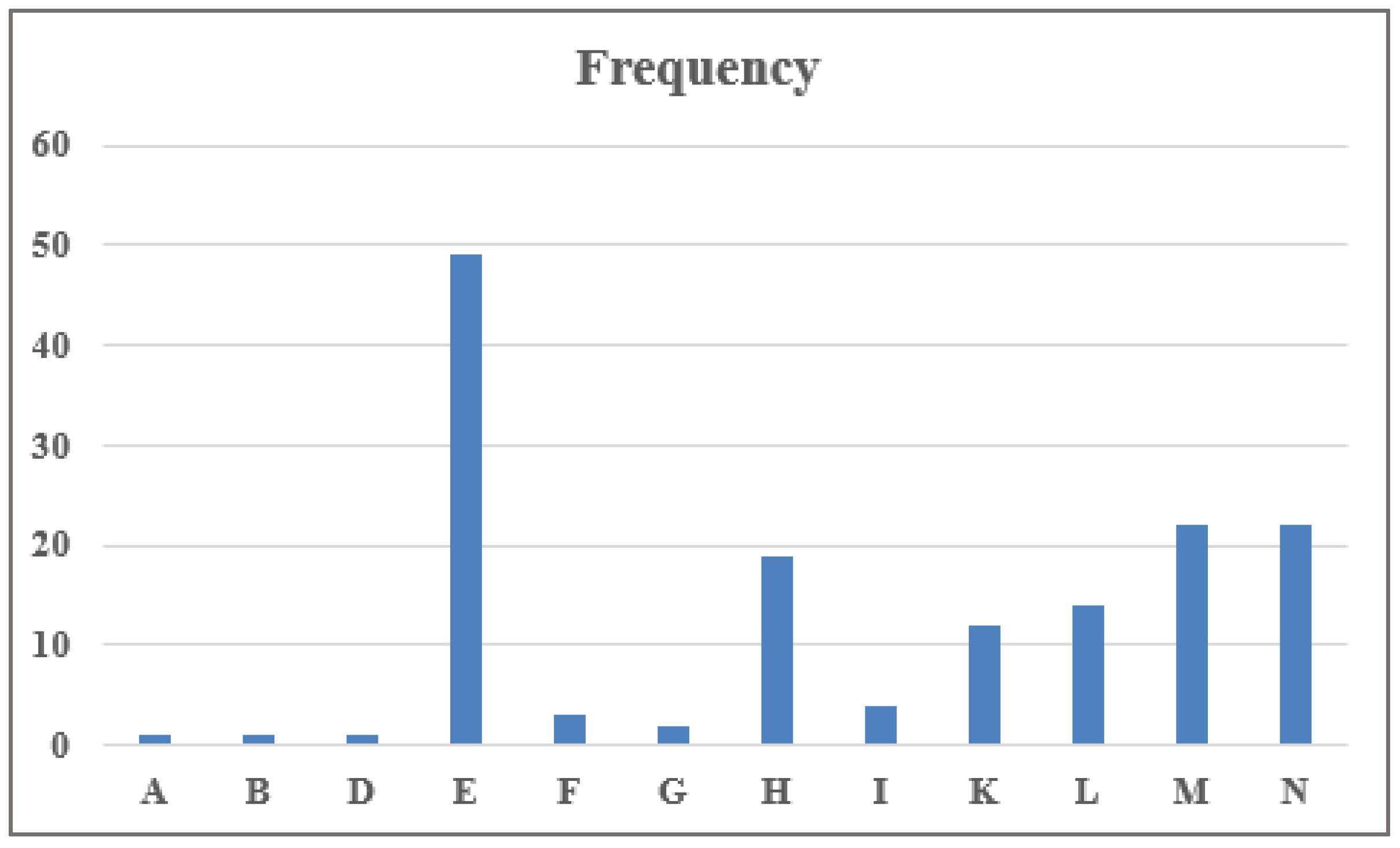
	CEFGHIKM	98.5%	E_NDRE3	E_B11	M_NDRE3	M_LSWI	E_LSWI	M_VIgreen	K_B11	G_B11	M_NDRE2	H_RESI

shows the top10 optimal feature sets of the best combination types for soybeans identification in each period. The best temporal combinations for soybean on 8 May, 12 June, and 7 July were the same as those for corn. The maximum identification accuracies achieved using A, CDHIJ, and BEFHIM were 63%, 81.8%, and 98.5%, respectively. On 13 May, the maximum soybean identification accuracy (70%) was achieved using three combinations of ABF, while on 28 May, the maximum identification accuracy (76.2%) was achieved using three combinations of AFG. On 7 July, the maximum identification accuracy for each combination was above 94% to achieve the soybean early identification accuracy. Figure 13 shows the frequency of key change temporal in the top10 feature sets of all the best combination types for soybeans in this period. The frequency of E is the highest, followed by M, N, and H. Adding these different time phases can effectively capture soybean growth information and enable them to be identified effectively.

5. Discussion

(1) Potential of using crop growth difference information for early identification

Currently, remote sensing recognition of crops is mainly based on all available images acquired throughout the growth period [68,69,70]. However, the limited imagery available in the early growth stages poses a great challenge to early crop identification [71]. The paper investigated the impact of using differential temporal information for early crop identification. Specifically, a dataset of early-stage growth characteristics was constructed based on differences in spectral features among all available temporal phases of the crop at each period, and all possible combinations of each period were identified. The results show that the different time phase features, such as mid-May and late April (F), are more critical for the early identification of rice; for the early identification of corn, the difference time phase features, such as early July and mid-June, late May, mid-May, and late May and late April (E, M, L, H) play a key role in its early identification; for the early identification of soybeans, the difference time phases features such as early July and mid-June, mid-May, early May, and late-May and late-April (E, M, N, H) contribute more to its early identification. In addition, we compared the F1 accuracy of each crop obtained by this method with that in the study [24]. They used Sentinel-2 remote sensing images to construct spectral and vegetation index feature sets of various crops in each growth period in an incremental manner. It investigated the early recognition of corn, rice, and soybean in Northeast China based on common classifiers. As can be seen from

Table 13. Comparison of F1 identification accuracy of rice in 2020.

Period to	Proposed Method	Study [24]
8 May	83.8%	76.2%
13 May	94.6%	80%

,

Table 14. Comparison of F1 identification accuracy of corn in 2020.

Period to	Proposed Method	Study [24]
8 May	67.1%	61.5%
13 May	71.7%	63.3%
28 May	76.8%	63.9%
12 June	82%	56.1%
7 July	98.2%	83.9%

and

Table 15. Comparison of F1 identification accuracy of soybeans in 2020.

Period to	Proposed Method	Study [24]
8 May	63%	57.4%
13 May	70%	54.1%
28 May	76.2%	59.1%
12 June	81.8%	55.9%
7 July	98.5%	98.4%

, compared with [24], the recognition accuracy of crops at each stage obtained by our method is higher than that in this paper, mainly because the index we designed that can effectively highlight the crop growth characteristics, which comprehensively considers crop growth difference information and the time phase information, and can effectively amplify the difference between crops and distinguish them effectively. Therefore, the combination of spectral vegetation index features of crops with differential temporal features can effectively improve crop recognition accuracy at early growth stages.

(2) Effective identification features of crops at different periods

The use of suitable classification features can effectively improve the accuracy of remote sensing crop recognition [72,73,74,75]. Many studies have shown that spectral and vegetation indices derived from Sentinel-2 multispectral remote sensing images play a more important role in crop identification than spatial texture information in Northeast China [34,76]. Accordingly, this study selected ten spectral and 22 vegetation indices as image features and explored their differences for use in crop identification in different growth periods. We found that rice moisture information was more prominent in May and June, and some of the relevant vegetation indices constructed with short-wave infrared as input were more sensitive to the vegetation canopy moisture information [77], which could effectively capture the moisture information of rice and thus identify rice as early as possible. Corn and soybean are dryland crops with the same phenological period [78], and some indicators of low vegetation cover play a role in this period, but their recognition ability is limited. In July, when various crops enter their peak growth period, some indicators related to vegetation canopy cover and the red edge index can be fully utilized [72,79] to effectively identify corn and soybeans.

(3) Comparison of the performance of different classifiers in early crop identification

In this study, four common classifiers were selected to evaluate their recognition effectiveness in the early stage of crops. These classifiers were selected based on their wide application in land cover [80,81].

Table 16. Accuracy of rice identification in 2020 different periods.

Period to	Cart	GBDT	RF	SVM
8 May	73.2%	83.8%	83.7%	82.6%
13 May	90.9%	94.6%	96.8%	91.9%

,

Table 17. Accuracy of corn identification in 2020 different periods.

Period to	Cart	GBDT	RF	SVM
8 May	57.8%	67.1%	66.8%	60%
13 May	63.8%	71.7%	70.2%	76.8%
28 May	70.9%	76.2%	76.8%	72.9%
12 June	75.8%	82.1%	82.1%	80.2%
7 July	97.5%	98.2%	98.2%	97.9%

and

Table 18. Accuracy of soybeans identification in 2020 different periods.

Period to	Cart	GBDT	RF	SVM
8 May	54.8%	63.1%	61.7%	61.5%
13 May	60.3%	70%	67.3%	66.7%
28 May	69.8%	75.5%	76.3%	73.9%
12 June	75.2%	81.8%	81.7%	80.7%
7 July	96.7%	98.4%	98.2%	94.8%

summarize the F1 recognition accuracy of each crop at different periods. RF can achieve a maximum rice identification accuracy of 96.8% as early as 13 May, while the accuracy of GBDT is about 2% lower and SVM and Cart are about 5.8% lower. Both GBDT and RF reached 98% accuracy for corn and soybeans as early as 7 July, while Cart and SVM were lower, at around 97% for corn and 96.7% and 94.8% for soybeans, respectively. Overall, with the addition of more temporal features, the recognition accuracy of the four classifiers tended to increase, with GBDT and RF achieving better results in identifying the three crops in the early stage.

6. Conclusions

This study constructed a dataset of early crop growth characteristics based on temporal phase difference feature information and explored its potential for use in early crop recognition in typical black soil areas of Northeast China. Firstly, a multi-temporal crop growth characteristics dataset was constructed using the different information on crops in different periods of the early stages. Then, the feature optimization method was used to select the best feature set for all possible combinations in each period, and the early key identification characteristics of different crops and their stage change characteristics were explored. Finally, the performance differences of four classifiers in early crop recognition and the recognition accuracy levels of crops in different periods were analyzed. The conclusions are as follows:

(1) The early crop growth method proposed in this study is intuitive and easy to understand. It can effectively amplify the differences between early-stage crops and improve the accuracy of crop identification. Therefore, it has great potential in the early identification of crops. It can also quickly and accurately map the crop in its early stages, providing information reference for relevant agricultural departments and having practical solid application value.

(2) The difference time phase feature can distinguish between crops and improve their identification accuracy in the early stage. Rice changed obviously between mid-May and late April (F) periods; corn changed more obviously between early July and mid-June, late May, mid-May, and late May and late April, which were periods E, M, L, H; soybean changed more obviously between early July and mid-June, mid-May, early May, and late-May and late-April, which were periods E, M, N, H.

(3) Short-wave infrared bands and vegetation index feature sensitivity to water information, and low vegetation coverage contributed more to the early identification of rice, such as LSWI, SR, B11, and NDTI. For corn and soybean, short-wave infrared band, red-edge index, and vegetation canopy cover indicators were key in identifying both, such as B11, NDRE3, LSWI, VIgreen, RESI, and NDRE2.

(4) Corn can be identified as early as 7 July, with both PA and UA above 97%; soybean can be identified as early as 7 July, with both above 94%; and rice can be identified as early as 8 May, with both above 90%.

(5) GBDT and RF performed comparably in crop recognition, followed by SVM, while the Cart classifier was poorer.

References

1. Atzberger, C. Advances in Remote Sensing of Agriculture: Context Description, Existing Operational Monitoring Systems and Major Information Needs. Remote Sens. 2013, 5, 949–981. [Google Scholar] [CrossRef]
2. Chen, Z.; Ren, J.; Tang, H.; Shi, Y.; Liu, J. Progress and perspectives on agricultural remote sensing research and applications in China. J. Remote Sens. 2016, 20, 748–767. [Google Scholar]
3. Jia, K.; Li, Q.Z. Research status and prospect of feature variable selection for crop remote sensing classification. Resour. Sci. 2013, 35, 2507–2516. [Google Scholar]
4. Zhao, H.; Chen, Z.; Jiang, H.; Jing, W.; Sun, L.; Feng, M. Evaluation of Three Deep Learning Models for Early Crop Classification Using Sentinel-1A Imagery Time Series—A Case Study in Zhanjiang, China. Remote Sens. 2019, 11, 2673. [Google Scholar] [CrossRef]
5. You, N.S.; Dong, J.W. Examining earliest identifiable timing of crops using all available Sentinel 1/2 imagery and Google Earth Engine. ISPRS J. Photogramm. Remote Sens. 2020, 161, 109–123. [Google Scholar] [CrossRef]
6. Tian, H.; Chen, T.; Li, Q.; Mei, Q.; Wang, S.; Yang, M.; Wang, Y.; Qin, Y. A Novel Spectral Index for Automatic Canola Mapping by Using Sentinel-2 Imagery. Remote Sens. 2022, 14, 1113. [Google Scholar] [CrossRef]
7. Kang, Y.; Hu, X.; Meng, Q.; Zou, Y.; Zhang, L.; Liu, M.; Zhao, M. Land Cover and Crop Classification Based on Red Edge Indices Features of GF-6 WFV Time Series Data. Remote Sens. 2021, 13, 4522. [Google Scholar] [CrossRef]
8. Hu, Q.; Wu, W.B.; Song, Q.; Lu, M.; Chen, D.; Yu, Q.Y.; Tang, H.J. How do temporal and spectral features matter in crop classification in Heilongjiang Province, China? J. Integr. Agric. 2017, 16, 324–336. [Google Scholar] [CrossRef]
9. Rahmati, A.; Zoej, M.J.V.; Dehkordi, A.T. Early Identification of Crop Types Using Sentinel-2 Satellite Images and an Incremental Multi-Feature Ensemble Method (Case Study: Shahriar, Iran). Adv. Space Res. 2022, 70, 907–922. [Google Scholar] [CrossRef]
10. Yi, Z.; Jia, L.; Chen, Q.; Jiang, M.; Zhou, D.; Zeng, Y. Early-Season Crop Identification in the Shiyang River Basin Using a Deep Learning Algorithm and Time-Series Sentinel-2 Data. Remote Sens. 2022, 14, 5625. [Google Scholar] [CrossRef]
11. Valero, S.; Arnaud, L.; Planells, M.; Ceschia, E. Synergy of Sentinel-1 and Sentinel-2 Imagery for Early Seasonal Agricultural Crop Mapping. Remote Sens. 2021, 13, 4891. [Google Scholar] [CrossRef]
12. Lv, S.; Xia, X.; Pan, Y. Optimization of Characteristic Phenological Periods for Winter Wheat Extraction Using Remote Sensing in Plateau Valley Agricultural Areas in Hualong, China. Remote Sens. 2023, 15, 28. [Google Scholar] [CrossRef]
13. Yang, X.; Zhang, B.; Chen, Z.; Bai, Y.; Chen, P. A Multi-Temporal Network for Improving Semantic Segmentation of Large-Scale Landsat Imagery. Remote Sens. 2022, 14, 5062. [Google Scholar] [CrossRef]
14. Wei, M.F.; Qiao, B.J.; Zhao, J.H.; Zuo, X.Y. The area extraction of winter wheat in mixed planting area based on Sentinel-2 a remote sensing satellite images. Int. J. Parallel Emergent Distrib. Syst. 2020, 35, 297–308. [Google Scholar] [CrossRef]
15. Zhang, H.X.; Wang, Y.J.; Shang, J.L.; Liu, M.X.; Li, Q.Z. Investigating the impact of classification features and classifiers on crop mapping performance in heterogeneous agricultural landscapes. Int. J. Appl. Earth Obs. Geoinf. 2021, 102, 102388. [Google Scholar] [CrossRef]
16. Chen, A.; Li, Y. Rice Recognition of Different Growth Stages Based on Sentinel-2 Images in Mountainous Areas of Southwest China. Nongye Gongcheng Xuebao/Trans. Chin. Soc. Agric. Eng. 2020, 36, 192–199. [Google Scholar]
17. Xing, H.; Chen, B.; Lu, M. A Sub-Seasonal Crop Information Identification Framework for Crop Rotation Mapping in Smallholder Farming Areas with Time Series Sentinel-2 Imagery. Remote Sens. 2022, 14, 6280. [Google Scholar] [CrossRef]
18. Zhang, R.; Shao, Z.; Huang, X.; Wang, J.; Li, D. Object Detection in UAV Images via Global Density Fused Convolutional Network. Remote Sens. 2020, 12, 3140. [Google Scholar] [CrossRef]
19. Wang, N.; Zhai, Y.; Zhang, L. Automatic Cotton Mapping Using Time Series of Sentinel-2 Images. Remote Sens. 2021, 13, 1355. [Google Scholar] [CrossRef]
20. Zang, Y.; Chen, X.; Chen, J.; Tian, Y.; Shi, Y.; Cao, X.; Cui, X. Remote Sensing Index for Mapping Canola Flowers Using MODIS Data. Remote Sens. 2020, 12, 3912. [Google Scholar] [CrossRef]
21. Dong, J.; Xiao, X.; Menarguez, M.A.; Zhang, G.; Qin, Y.; Thau, D.; Biradar, C.; Moore, B., III. Mapping paddy rice planting area in northeastern Asia with Landsat 8 images, phenology-based algorithm and Google Earth Engine. Remote Sens. Environ. 2016, 85, 142–154. [Google Scholar] [CrossRef] [PubMed]
22. Hao, P.; Chen, Z.; Tang, H.; Li, D.; Li, H. New Workflow of Plastic-Mulched Farmland Mapping using Multi-Temporal Sentinel-2 data. Remote Sens. 2019, 11, 1353. [Google Scholar] [CrossRef]
23. Tuvdendorj, B.; Zeng, H.; Wu, B.; Elnashar, A.; Zhang, M.; Tian, F.; Nabil, M.; Nanzad, L.; Bulkhbai, A.; Natsagdorj, N. Performance and the Optimal Integration of Sentinel-1/2 Time-Series Features for Crop Classification in Northern Mongolia. Remote Sens. 2022, 14, 1830. [Google Scholar] [CrossRef]
24. Wei, M.; Wang, H.; Zhang, Y.; Li, Q.; Du, X.; Shi, G.; Ren, Y. Investigating the Potential of Sentinel-2 MSI in Early Crop Identification in Northeast China. Remote Sens. 2022, 14, 1928. [Google Scholar] [CrossRef]
25. Ashourloo, D.; Shahrabi, H.S.; Azadbakht, M.; Rad, A.M.; Aghighi, H.; Matkan, A.A.; Radiom, S. A Novel Automatic Method for Alfalfa Mapping Using Time Series of Landsat-8 OLI Data. IEEE J. Sel. Top. Appl. Earth Obs. Remote. Sens. 2018, 11, 4478–4487. [Google Scholar] [CrossRef]
26. Dong, J.; Fu, Y.; Wang, J.; Tian, H.; Yuan, W. Early season mapping of winter wheat in China based on Landsat and Sentinel images. Earth Syst. Sci. Data 2020, 12, 3081–3095. [Google Scholar] [CrossRef]
27. Zhang, H.; Du, H.; Zhang, C.; Zhang, L. An automated early-season method to map winter wheat using time-series Sentinel-2 data: A case study of Shandong, China. Comput. Electron. Agric. 2021, 182, 105962. [Google Scholar] [CrossRef]
28. Li, F.; Ren, J.; Wu, S.; Zhao, H.; Zhang, N. Comparison of Regional Winter Wheat Mapping Results from Different Similarity Measurement Indicators of NDVI Time Series and Their Optimized Thresholds. Remote Sens. 2021, 13, 1162. [Google Scholar] [CrossRef]
29. He, S.; Peng, P.; Chen, Y.; Wang, X. Multi-Crop Classification Using Feature Selection-Coupled Machine Learning Classifiers Based on Spectral, Textural and Environmental Features. Remote Sens. 2022, 14, 3153. [Google Scholar] [CrossRef]
30. Qiu, B.W.; Chen, C.C. Mapping Staple Crops in China from Time Series Satellite Images; China Science Pulishing & Media Ltd.(CSPM): Beijing, China, 2022; ISBN 978-7-03-071864-8. [Google Scholar]
31. Zhang, H.; Kang, J.; Xu, X.; Zhang, L. Accessing the temporal and spectral features in crop type mapping using multi-temporal Sentinel-2 imagery: A case study of Yi’an County, Heilongjiang province, China. Comput. Electron. Agric. 2020, 176, 105618. [Google Scholar] [CrossRef]
32. Gholamrezaie, H.; Hasanlou, M.; Amani, M.; Mirmazloumi, S.M. Automatic Mapping of Burned Areas Using Landsat 8 Time-Series Images in Google Earth Engine: A Case Study from Iran. Remote Sens. 2022, 14, 6376. [Google Scholar] [CrossRef]
33. Shen, J.; Tao, C.; Qi, J.; Wang, H. Semi-Supervised Convolutional Long Short-Term Memory Neural Networks for Time Series Land Cover Classification. Remote Sens. 2021, 13, 3504. [Google Scholar] [CrossRef]
34. Li, B.; Liu, K.; Wang, M.; He, Q.; Jiang, Z.; Zhu, W.; Qiao, N. Global Dynamic Rainfall-Induced Landslide Susceptibility Mapping Using Machine Learning. Remote Sens. 2022, 14, 5795. [Google Scholar] [CrossRef]
35. Zhao, L.C. Research on Indicative Image Identification Feature of Major Crops and Its Application Method. Master’s Thesis, Aerospace Information Research Institute Chine Academy of Sciences, Beijing, China, 2020. [Google Scholar]
36. Rouse, J.W.; Haas, R.H.; Schell, J.A.; Deering, D.W. Monitoring the Vernal Advancement and Retrogradation (Green Wave Effect) of Natural Vegetation; Remote Sensing Center: College Station, TX, USA, 1973. [Google Scholar]
37. Xiao, X.; Boles, S.; Frolking, S.; Li, C.; Babu, J.Y.; Salas, W.; Moore, B., III. Mapping paddy rice agriculture in South and Southeast Asia using multi-temporal MODIS images. Remote Sens. Environ. 2006, 100, 95–113. [Google Scholar] [CrossRef]
38. Huete, A.; Justice, C.; Van Leeuwen, W. MODIS vegetation index (MOD13). Algorithm Theor. Basis Doc. 1999, 3, 295–309. [Google Scholar]
39. Xiao, C.; Peng, L.; Feng, Z.; Liu, Y.; Zhang, X.Z. Sentinel-2 red-edge spectral indices (RESI) suitability for mapping rubber boom in Luang Namtha Province, northern Lao PDR. Int. J. Appl. Earth Obs. Geoinf. 2020, 93, 102176. [Google Scholar] [CrossRef]
40. Gitelson, A.; Merzlyak, M.N. Quantitative estimation of chlorophyll-a using reflectance spectra: Experiments with autumn chestnut and maple leaves. J. Photochem. Photobiol. B Biol. 1994, 22, 247–252. [Google Scholar] [CrossRef]
41. Vogelmann, J.E.; Rock, B.N.; Moss, D.M. Red edge spectral measurements from sugar maple leaves. Int. J. Remote Sens. 1993, 14, 1563–1575. [Google Scholar] [CrossRef]
42. Peddle, D.R.; Hall, F.G.; Ledrew, E.F. Remote Sensing of Boreal Forest Biophysical Variables using Spectral Mixture Analysis and a Canopy Reflectance Model. In Proceedings of the 26th International Symposium on Remote Sensing of Environment, Vancouver, BC, Canada, 25 March 1996. [Google Scholar]
43. Maire, G.L.; François, C.; Dufrêne, E. Towards universal broad leaf chlorophyll indices using PROSPECT simulated database and hyperspectral reflectance measurements. Remote. Sens. Environ. 2004, 89, 1–28. [Google Scholar] [CrossRef]
44. Peña-Barragán, J.M.; Ngugi, M.K.; Plant, R.E.; Six, J. Object-based crop identification using multiple vegetation indices, textural features and crop phenology. Remote Sens. Environ. 2011, 115, 1301–1316. [Google Scholar] [CrossRef]
45. Rondeaux, G.; Steven, M.; Baret, F. Optimization of soil-adjusted vegetation indices. Remote Sens. Environ. 1996, 55, 95–107. [Google Scholar] [CrossRef]
46. Deventer, V.A.P.; Ward, A.D.; Gowda, P.H.; Lyon, J.G. Using thematic mapper data to identify contrasting soil plains and tillage practices. Photogramm. Eng. Remote Sens. 1997, 63, 87–93. [Google Scholar]
47. Chen, J.M. Evaluation of Vegetation Indices and a Modified Simple Ratio for Boreal Applications. Can. J. Remote Sens. 1996, 22, 229–242. [Google Scholar] [CrossRef]
48. Carrasco, L.; Fujita, G.; Kito, K.; Miyashita, T. Historical mapping of rice fields in Japan using phenology and temporally aggregated Landsat images in Google Earth Engine. ISPRS J. Photogramm. Remote Sens. 2022, 191, 277–289. [Google Scholar] [CrossRef]
49. Yang, H.; Pan, B.; Li, N.; Wang, W.; Zhang, J.; Zhang, X. A systematic method for spatio-temporal phenology estimation of paddy rice using time series Sentinel-1 images. Remote Sens. Environ. 2021, 259, 112394. [Google Scholar] [CrossRef]
50. Hu, Q.; Sulla-Menashe, D.; Xu, B.; Yin, H.; Wu, W. A phenology-based spectral and temporal feature selection method for crop mapping from satellite time series. Int. J. Appl. Earth Obs. Geoinf. 2019, 80, 218–229. [Google Scholar] [CrossRef]
51. Cai, Y.; Guan, K.; Jian, P.; Wang, S.; Zhan, L. A high-performance and in-season classification system of field-level crop types using time-series Landsat data and a machine learning approach. Remote Sens. Environ. 2018, 210, 35–47. [Google Scholar] [CrossRef]
52. Vska, B.; Jk, C.; Wwh, D.; Fmhb, E.; Arg, A. Mapping crops within the growing season across the United States. Remote Sens. Environ. 2020, 251, 112048. [Google Scholar]
53. Weilandt, F.; Behling, R.; Goncalves, R.; Madadi, A.; Richter, L.; Sanona, T.; Spengler, D.; Welsch, J. Early Crop Classification via Multi-Modal Satellite Data Fusion and Temporal Attention. Remote Sens. 2023, 15, 799. [Google Scholar]
54. Kiala, Z.; Odindi, J.; Mutanga, O. Determining the Capability of the Tree-Based Pipeline Optimization Tool (TPOT) in Mapping Parthenium Weed Using Multi-Date Sentinel-2 Image Data. Remote Sens. 2022, 14, 1687. [Google Scholar] [CrossRef]
55. Ramezan, C.A. Transferability of Recursive Feature Elimination (RFE)-Derived Feature Sets for Support Vector Machine Land Cover Classification. Remote Sens. 2022, 14, 6218. [Google Scholar] [CrossRef]
56. Zhou, X.; Wang, J.; He, Y.; Shan, B. Crop Classification and Representative Crop Rotation Identifying Using Statistical Features of Time-Series Sentinel-1 GRD Data. Remote Sens. 2022, 14, 5116. [Google Scholar]
57. Asam, S.; Gessner, U.; Almengor González, R.; Wenzl, M.; Kriese, J.; Kuenzer, C. Mapping Crop Types of Germany by Combining Temporal Statistical Metrics of Sentinel-1 and Sentinel-2 Time Series with LPIS Data. Remote Sens. 2022, 14, 2981. [Google Scholar] [CrossRef]
58. Dobrinić, D.; Gašparović, M.; Medak, D. Sentinel-1 and 2 Time-Series for Vegetation Mapping Using Random Forest Classification: A Case Study of Northern Croatia. Remote Sens. 2021, 13, 2321. [Google Scholar] [CrossRef]
59. Yang, L.; Mansaray, L.R.; Huang, J.; Wang, L. Optimal Segmentation Scale Parameter, Feature Subset and Classification Algorithm for Geographic Object-Based Crop Recognition Using Multisource Satellite Imagery. Remote Sens. 2019, 11, 514. [Google Scholar] [CrossRef]
60. Xiao, T.; Liu, H.; Cheng, Y. Corn Disease Identification Based on improved GBDT Method. In Proceedings of the 2019 6th International Conference on Information Science and Control Engineering (ICISCE), Shanghai, China, 20–22 December 2019; pp. 215–219. [Google Scholar]
61. Serbouti, I.; Raji, M.; Hakdaoui, M.; El Kamel, F.; Pradhan, B.; Gite, S.; Alamri, A.; Maulud, K.N.A.; Dikshit, A. Improved Lithological Map of Large Complex Semi-Arid Regions Using Spectral and Textural Datasets within Google Earth Engine and Fused Machine Learning Multi-Classifiers. Remote Sens. 2022, 14, 5498. [Google Scholar]
62. Basheer, S.; Wang, X.; Farooque, A.A.; Nawaz, R.A.; Liu, K.; Adekanmbi, T.; Liu, S. Comparison of Land Use Land Cover Classifiers Using Different Satellite Imagery and Machine Learning Techniques. Remote Sens. 2022, 14, 4978. [Google Scholar] [CrossRef]
63. Ioannidou, M.; Koukos, A.; Sitokonstantinou, V.; Papoutsis, I.; Kontoes, C. Assessing the Added Value of Sentinel-1 PolSAR Data for Crop Classification. Remote Sens. 2022, 14, 5739. [Google Scholar]
64. Croci, M.; Impollonia, G.; Blandinières, H.; Colauzzi, M.; Amaducci, S. Impact of Training Set Size and Lead Time on Early Tomato Crop Mapping Accuracy. Remote Sens. 2022, 14, 4540. [Google Scholar] [CrossRef]
65. Wang, X.; Zhang, J.; Xun, L.; Wang, J.; Wu, Z.; Henchiri, M.; Zhang, S.; Zhang, S.; Bai, Y.; Yang, S.; et al. Evaluating the Effectiveness of Machine Learning and Deep Learning Models Combined Time-Series Satellite Data for Multiple Crop Types Classification over a Large-Scale Region. Remote Sens. 2022, 14, 2341. [Google Scholar] [CrossRef]
66. Jiang, H.; Li, D.; Jing, W.; Xu, J.; Huang, J.; Yang, J.; Chen, S. Early Season Mapping of Sugarcane by Applying Machine Learning Algorithms to Sentinel-1A/2 Time Series Data: A Case Study in Zhanjiang City, China. Remote Sens. 2019, 11, 861. [Google Scholar] [CrossRef]
67. Meng, S.; Zhong, Y.; Luo, C.; Hu, X.; Wang, X.; Huang, S. Optimal Temporal Window Selection for Winter Wheat and Rapeseed Mapping with Sentinel-2 Images: A Case Study of Zhongxiang in China. Remote Sens. 2020, 12, 226. [Google Scholar] [CrossRef]
68. Shen, Y.; Li, Q.Z.; Du, X.; Wang, H.Y.; Zhang, Y. Indicative features for identifying corn and soybean using remote sensing imagery at middle and later growth season. Natl. Remote Sens. Bull. 2022, 26, 1410–1422. [Google Scholar]
69. Zhong, B.; Yang, A.; Jue, K.; Wu, J. Long Time Series High-Quality and High-Consistency Land Cover Mapping Based on Machine Learning Method at Heihe River Basin. Remote Sens. 2021, 13, 1596. [Google Scholar] [CrossRef]
70. Tian, Q.J.; Min, X.J. Advances in study on vegetation indices. Adv. Earth Sci. 1998, 13, 327–333. [Google Scholar]
71. Valero, S.; Ceccato, P.; Baethgen, W.E.; Chanussot, J. Identification of agricultural crops in early stages using remote sensing images. In Proceedings of the 2013 IEEE International Geoscience and Remote Sensing Symposium—IGARSS, Melbourne, VIC, Australia, 21–26 July 2013; pp. 4229–4232. [Google Scholar]
72. Inglada, J.; Vincent, A.; Arias, M.; Marais-Sicre, C. Improved Early Crop Type Identification by Joint Use of High Temporal Resolution SAR And Optical Image Time Series. Remote Sens. 2016, 8, 362. [Google Scholar] [CrossRef]
73. Luo, H.; Li, M.; Dai, S.; Li, H.; Li, Y.; Hu, Y.; Zheng, Q.; Yu, X.; Fang, J. Combinations of Feature Selection and Machine Learning Algorithms for Object-Oriented Betel Palms and Mango Plantations Classification Based on Gaofen-2 Imagery. Remote Sens. 2022, 14, 1757. [Google Scholar] [CrossRef]
74. Liao, Q. Intelligent classification model of land resource use using deep learning in remote sensing images. Ecol. Model. 2023, 475, 110231. [Google Scholar]
75. Wang, L.; Wang, J.; Liu, Z.; Zhu, J.; Qin, F. Evaluation of a deep-learning model for multispectral remote sensing of land use and crop classification. Crop J. 2022, 10, 1435–1451. [Google Scholar] [CrossRef]
76. Luo, C.; Qi, B.; Liu, H.; Guo, D.; Lu, L.; Fu, Q.; Shao, Y. Using Time Series Sentinel-1 Images for Object-Oriented Crop Classification in Google Earth Engine. Remote Sens. 2021, 13, 561. [Google Scholar] [CrossRef]
77. Di, Y.; Zhang, G.; You, N.; Yang, T.; Zhang, Q.; Liu, R.; Doughty, R.B.; Zhang, Y. Mapping Croplands in the Granary of the Tibetan Plateau Using All Available Landsat Imagery, A Phenology-Based Approach, and Google Earth Engine. Remote Sens. 2021, 13, 2289. [Google Scholar]
78. Yaramasu, B.; Bandaru, B.; Pnvr, K. Pre-season crop type mapping using deep neural networks. Comput. Electron. Agric. 2020, 176, 105664. [Google Scholar] [CrossRef]
79. Sigurdsson, J.; Armannsson, S.E.; Ulfarsson, M.O.; Sveinsson, J.R. Fusing Sentinel-2 and Landsat 8 Satellite Images Using a Model-Based Method. Remote Sens. 2022, 14, 3224. [Google Scholar] [CrossRef]
80. Wen, C.; Lu, M.; Song, Q.; Chen, R.; Zhang, S. A comparative analysis of feature extraction and classifiers for crop classification based on time series data. China Agric. Inform. 2021, 33, 1–16. [Google Scholar]
81. Zhang, N.; Chen, M.; Yang, F.; Yang, C.; Yang, P.; Gao, Y.; Shang, Y.; Peng, D. Forest Height Mapping Using Feature Selection and Machine Learning by Integrating Multi-Source Satellite Data in Baoding City, North China. Remote Sens. 2022, 14, 4434. [Google Scholar] [CrossRef]
Figure 1. The geographical location of the region.
Remotesensing 15 00853 g001
Figure 2. Workflow for early crop identification based on multi-temporal difference information.
Remotesensing 15 00853 g002
Figure 3. The mean spectral values of the three crops at different periods. (a) The mean spectral values of corn at different periods, (b) The mean spectral values of soybean at different periods, and (c) The mean spectral values of rice at different periods.
Remotesensing 15 00853 g003
Figure 4. Diagram of the multi-temporal crop discrimination information in the 2020 crop early stage.
Remotesensing 15 00853 g004
Figure 5. Maximum OA changes of the classifiers in 2020 different periods.
Remotesensing 15 00853 g005
Figure 6. Maximum kappa coefficient changes of the classifiers in 2020 different periods.
Remotesensing 15 00853 g006
Figure 7. Optimal identification results in 2020 different periods. (a) Identification results on 8 May; (b) Identification results on 13 May; (c) Identification results on 28 May; (d) Identification results on 12 June; (e) Identification results on 7 July.
Remotesensing 15 00853 g007
Figure 8. Percentage of different character types of rice in 2020 different periods.
Remotesensing 15 00853 g008
Figure 9. Frequency of the key change temporal on 13 May 2020.
Remotesensing 15 00853 g009
Figure 10. Percentage of different character types of corn in 2020 different periods.
Remotesensing 15 00853 g010aRemotesensing 15 00853 g010b
Figure 11. Frequency of the key change temporal on 7 July 2020.
Remotesensing 15 00853 g011
Figure 12. Percentage of different character types of soybeans in 2020 different periods.
Remotesensing 15 00853 g012aRemotesensing 15 00853 g012b
Figure 13. Frequency of the key change temporal on 7 July 2020.
Remotesensing 15 00853 g013