Article

A GNSS/LiDAR/IMU Pose Estimation System Based on Collaborative Fusion of Factor Map and Filtering

1
Key Laboratory of 3D Information Acquisition and Application, MOE, Capital Normal University, Beijing 100048, China
2
Base of the State Key Laboratory of Urban Environmental Process and Digital Modeling, Capital Normal University, Beijing 100048, China
3
College of Resource Environment and Tourism, Capital Normal University, Beijing 100048, China
4
Neolix Technologies Co., Ltd., Beijing 100016, China
5
School of Vehicle and Mobility, Tsinghua University, Beijing 100084, China
6
Institute of Computing Technology, Chinese Academy of Sciences, Beijing 100045, China
*
Author to whom correspondence should be addressed.
These authors contributed equally to this work.
Remote Sens. 2023, 15(3), 790; https://doi.org/10.3390/rs15030790
Submission received: 10 December 2022 / Revised: 23 January 2023 / Accepted: 25 January 2023 / Published: 30 January 2023

Abstract

:
One of the core issues of mobile measurement is the pose estimation of the carrier. The classic Global Navigation Satellite System/Inertial Measurement Unit (GNSS/IMU) integrated navigation scheme has high positioning accuracy but is vulnerable to Global Navigation Satellite System (GNSS) signal occlusion and multipath effect. Simultaneous Localization and Mapping (SLAM) is not affected by signal occlusion, but there are problems such as error accumulation and scene degradation. The multi-sensor fusion scheme combining the two technologies can effectively expand the scene coverage and improve the positioning accuracy and system robustness. However, the current scheme has some limitations. On the one hand, GNSS plays a less important role in most SLAM systems, only for initialization or as a closed-loop factor and other auxiliary work. On the other hand, in the fusion method, most of the current systems only use filtering or graph optimization, without taking into account the advantages of both. Aiming at pose estimation for mobile carriers, this paper combines the advantages of the global optimization of the factor graph and the local optimization of filtering and proposes a GNSS-IMU-LiDAR Constraint Kalman Filter (abbreviated as GIL-CKF), which has the characteristics of full coverage and effectively improving absolute accuracy and high output frequency. The scheme proposed in this paper consists of three parts. Firstly, an extensible factor map is used to fuse the positioning information from different sources, including GNSS, IMU, LiDAR, and a closed-loop map, to maintain a high-precision SLAM system, and the output is used as Multi-Sensor-Fusion-Odometry (MSFO). Then, the scene is divided according to the GNSS quality factor, and a Scene Optimizer (SO) is designed to filter GNSS pose and MSFO. Finally, the results are input into the Extended Kalman Filter (EKF) together with the original IMU data for further optimization and smoothing. The experimental results show that the integration of high-precision GNSS positioning information with IMU, LiDAR, a closed-loop map, and other information through the factor map can effectively suppress error accumulation and improve the overall accuracy of the SLAM system. The SO based on GNSS indicators can fully retain high-precision GNSS positioning information, effectively play their respective advantages of filtering and graph optimization, and alleviate the conflict between global and local optimization. SO with EKF filtering furthers optimization, can improve the output frequency, and smooth the trajectory. GIL-CKF can effectively improve the accuracy and robustness of pose estimation and has obvious advantages in multi-sensor scene complementarity, partial road section accuracy improvement, and high input frequency.

1. Introduction

Compared with traditional station measurement, the Mobile Mapping System (MMS) realizes dynamic measurement, avoids manual handling and installation between stations, and greatly improves production efficiency and operation freedom [1]. The realization of Mobile Mapping measurement depends on the positioning navigation unit. Therefore, ensuring the accurate positioning of sensors in motion is the premise of the effective implementation of mobile measurement. GNSS/IMU integrated navigation technology is a classic positioning navigation scheme for mobile measurement that has been widely used in the surveying and mapping industries and achieved good results. In high-precision measurement, centimeter-level dynamic positioning can be achieved by using DGNSS (Differential GNSS)/IMU integrated navigation based on differential carrier phase observations [2,3,4]. However, GNSS is difficult to obtain as a fixed solution in weak signal areas, and positioning accuracy degrades to decimeter or even meter levels [5]. Simultaneous Localization and Mapping (SLAM) is a popular solution to the positioning problem in weak GNSS signal environments. The principle of SLAM is to establish the surrounding environment model by using lasers, cameras, and other sensors and to estimate its motion state by calculating the relative relationship between the current observation point and the environment [1,6,7,8,9,10].
SLAM technology and GNSS/IMU integrated navigation technology are effectively complementary in the scene, which provides the possibility for accurate pose estimation in a wide range of scenarios. A large number of researchers have conducted a lot of work on how to combine the two. Based on GNSS/IMU integrated navigation technology, some scholars try to introduce the relative positioning information of LiDAR to make up for the deficiency of weak GNSS signal area positioning. A direct method is using LiDAR/IMU as a supplement to GNSS in weak GNSS signal environments, such as indoors and within cities. LiDAR and GNSS alternated to assist the IMU in providing integrated navigation results, which constituted a GNSS/IMU/LiDAR integrated navigation system [11]. When the GNSS signal is good, SLAM is used to synchronously observe, locate, and update the three-dimensional position of the environmental feature mark. When the GNSS signal is blocked, the position estimation of the carrier is obtained by the relative relationship between the carrier and the environmental feature mark, and the IMU parameters are corrected to suppress the IMU cumulative error [12]. Essentially, this type of work focuses on unifying the GNSS and SLAM coordinate systems. GNSS and SLAM are alternately used as the main odometers to expand the scene, but they are independent of each other. There is no information fusion, which is actually loosely coupled. In terms of a deeper information fusion, J. G. et al., use LiDAR/IMU to achieve relative positioning and mapping. When high-precision GNSS is available, GNSS information is used as the “loop” in SLAM to optimize the trajectory by global optimization [13]. This, to a certain extent, has improved the positioning accuracy of the SLAM system. More groundbreaking work is the tight coupling factor graph model [14,15], which incorporates GNSS and other multi-type positioning technologies as different probability factors into a probabilistic factor graph framework to obtain the global optimal solution by calculating the maximum posterior probability of the joint probability of all factors. Based on the factor graph model, an open-source optimization library called GTSAM was developed. Based on GTSAM, T. et al. further constructed a complete set of a multi-sensor factor graph fusion SLAM system called LIO-SAM [16]. Compared with those that are loosely coupled, this method combines GNSS high-precision global positioning information and SLAM relative positioning information closely through graph optimization, which inhibits the error accumulation of the SLAM system and achieves greater results. At the same time, Baidu proposes the MSF (Multi-Sensor Fusion) scheme, which takes GNSS, IMU, LiDAR, and visual cameras as sub-positioning information and fuses all of this information through an error-state Kalman filter [17]. The overall fusion realizes the error control of the pose estimation system and improves its robustness. This is a filtering fusion method that realizes Multi-Sensor Fusion at the information level and achieves better results.
Different sensors impose different constraints on the pose estimation of mobile platforms [18]. The Multi-Sensor Fusion scheme can integrate the advantages of various sensors and effectively improve the coverage of the scene and the robustness of the system, which has gradually become a trend [19,20,21,22]. The development process of Multi-Sensor Fusion technology shows the characteristics from loose to close, which is mainly divided into two different fusion architectures: filtering fusion and graph optimization fusion [23,24]. The former corresponds to the iterative process, which marginalizes the past pose and summarizes the information obtained over time with the probability distribution [18]. The calculation speed is fast, and the output frequency is high [23,24,25]. The latter recombines historical trajectory points and observation data, retains global constraints, and performs batch processing with a higher accuracy but a lower output frequency [20,23,24,26,27]. On the other hand, due to the Gaussian distribution assumption of sensor error and the inaccurate estimation of error covariance, the fusion results of the two sensors show a decrease in accuracy compared with the single sensor (such as GNSS). Therefore, both of them face the same challenge, namely, the conflict problem of local and global optimization [19].
Aiming at the goal of Multi-Sensor Fusion pose estimation on the basis of previous studies combined with scene complementary and information fusion methods, this paper proposes an extensible and robust fusion pose estimation scheme with high precision. The scheme includes a variety of positioning sensors and a set of fusion algorithms. The main idea is to prioritize the use of GNSS positioning information, and SLAM supplements the location of the unlocked region. Through the fusion algorithm, GNSS positioning information is introduced into the SLAM system to improve the positioning accuracy and stability of the SLAM system. In the algorithm structure, this paper uses an extensible factor graph to fuse the positioning information from different sources, such as GNSS, LiDAR, and IMU, to form a Multi-Sensor Fusion Odometry (MSFO) and uses a Scene Optimizer (SO) to select the GNSS pose and MSFO results. The selected results and IMU data are input into EKF filtering to further optimize and smooth them.

2. Materials and Methods

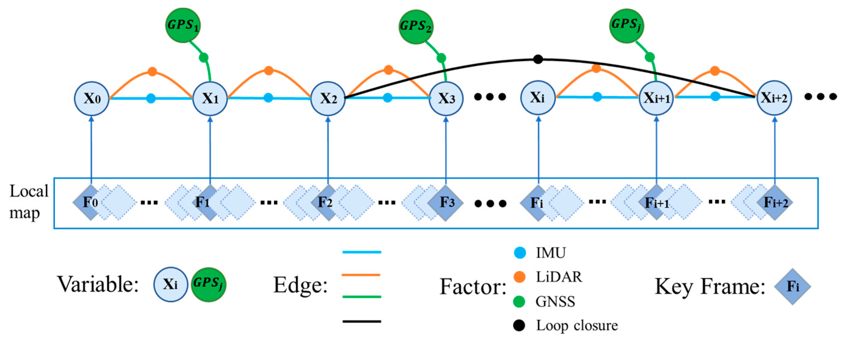
2.1. Factor Graph Optimization

The system receives input from a LiDAR, an IMU, and a GNSS. Four types of factors are introduced to construct the factor graph: (a) an IMU preintegration factor, (b) a lidar odometry factor, (c) a GPS factor, and (d) a loop closure factor. The application of these factors is discussed in Section 3.2.1. The factor graph is a Probabilistic Graphical Model (PGM). Formally, a factor graph is a bipartite graph with two types of nodes: F = ( U , V , ) , where U means factor nodes, V means variable nodes, and edge always exists between factor nodes and variable nodes [14,15,28]. The variables refer to the random variables in the optimization problem, namely pose, road sign, etc. There is a certain conditional probability relationship between these variables, which provides the basic probability information in the SLAM optimization problem. This probability information can be derived from observation or prior knowledge. This relationship is represented by edges, and the probability information of these variables is aggregated by a factor, which constitutes the factor graph representation of the optimization problem. The factor is essentially a likelihood factor, representing the likelihood relationship between two variables. Specifically, there is a Markov property between the adjacent poses of the LiDAR odometer, which can be expressed by a factor [15,28]. The observational relationship between any pose point and the observed landmark can be expressed by a factor. The synchronous positioning relationship between any pose point and GNSS observations can also be expressed by a factor, as shown in Figure 1. As a probabilistic model, the factor graph has been widely used in the field of SLAM. The strict mathematical definition of the factor graph can be seen in Professor Frank’s article [28].
The factor graph can effectively fuse IMU pre-integration, a LiDAR odometer, GNSS high-precision positioning information, and SLAM closed-loop information. This scheme mainly uses the factor graph in MSFO.

2.2. EKF Filter

EKF is an extended form of the standard Kalman filter in nonlinear problems. EKF expands the nonlinear function through the Taylor expansion to linearize the nonlinear function. It then approximates the state estimation and covariance estimation of the system by the Kalman filter algorithm to filter the signal [29,30].
EKF plays two important roles in our scheme. Firstly, it can improve the output frequency of the pose. Secondly, the update amount selected by the optimizer is switched back and forth between the GNSS pose and the LiDAR pose. Although the switching position is carefully selected, there will inevitably be slight differences. EKF can further optimize and smooth these parts.

3. Methodology

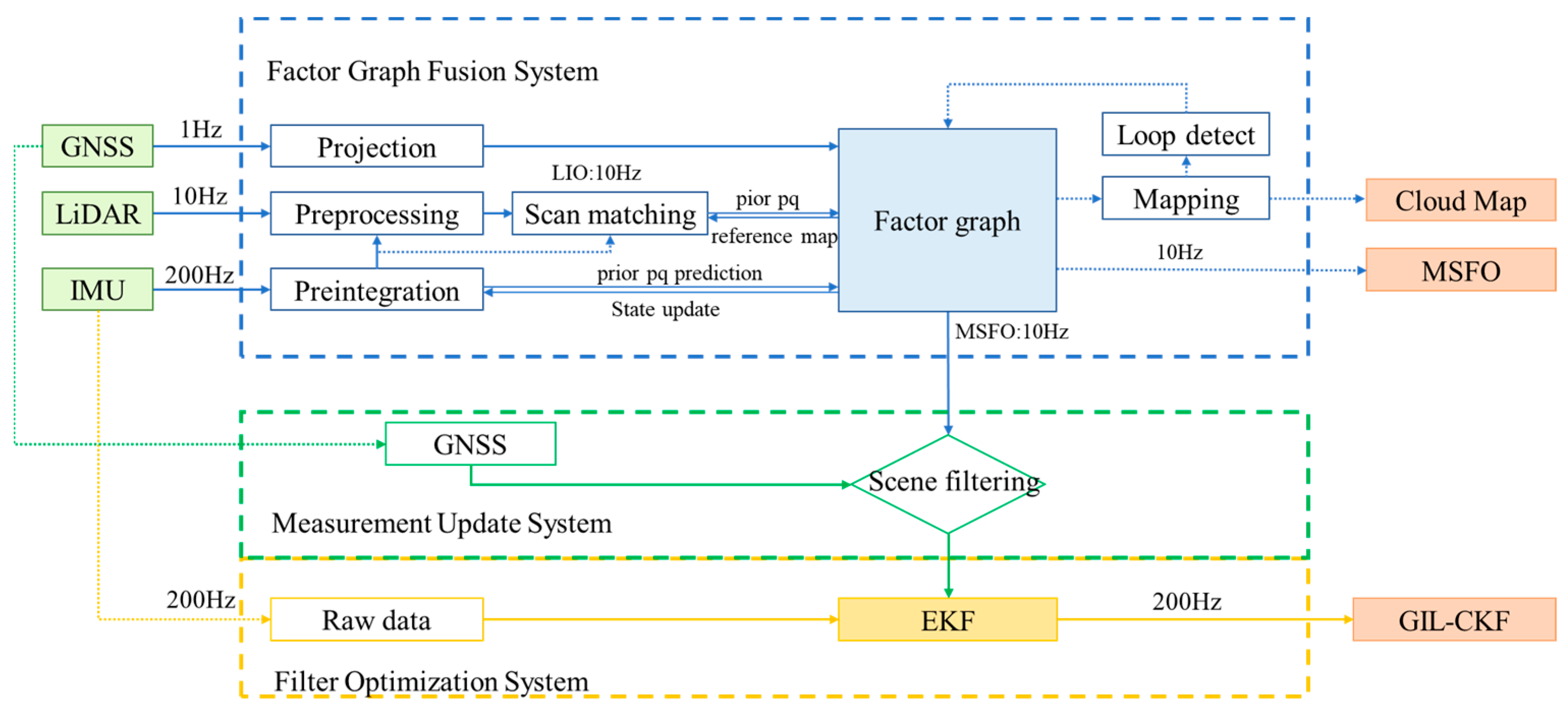
3.1. Technical Framework

In this paper, the device is built on the machine car. It consists of three hardware modules: IMU inertial measurement unit, GNSS, and LiDAR. The hardware is shown in Figure 2 and the detailed parameters are shown in Table 1.
The coordinate systems used in this paper are: the World Coordinate System (W), the IMU Coordinate System (B), and the LiDAR Coordinate System (L). This paper assumes that the IMU Coordinate System coincides with the Robot Coordinate System, and the carrier state x k is expressed as: x k = [ R , p , v ] , in which R   SO ( 3 ) is the rotation matrix, p     R 3 is position vector, and v represents the velocity.
The essence of Multi-Sensor Fusion optimization is to solve the probability of optimal distribution of pose information from multiple sensors and multiple moments; the key is the fusion model. In order to make full use of the high-precision positioning information of GNSS, the positioning ability of SLAM in weak GNSS signal areas, the error control ability of graph optimization fusion, and the high-frequency positioning ability of filtering fusion, this paper adopts the design idea of combining filtering and graph optimization to propose a GNSS/IMU/LiDAR multi-constrained filtering fusion system, referred to as GIL-CKF. This scheme adopts a two-step fusion strategy. First, a scalable factor graph is used to fuse positioning information from different sources, such as GNSS, LiDAR, IMU, etc., to form a Multi-Sensor Fusion Odometer (MSFO) to achieve overall accuracy control of the SLAM system. Second, in conjunction with scene filtering, MSFO and GNSS alternately update the IMU state in EKF filtering to further smooth and optimize the local trajectory. The technical framework is shown in Figure 3.
This scheme adopts the “prediction + update” filter structure as a whole, and the update amount is specially designed. The difference is that the update amount of MSCKF is based on the re-projection error of the same visual feature point on different graphs, and the graph optimization problem is constructed. The update amount of this scheme is calculated between multi-source sensors and closed-loop information. What is more, GNSS is directly selected as the update quantity in the open area, which guarantees the accuracy of the open area simply and effectively. In the open, unblocked area, differential GNSS can provide centimeter-level, high-precision positioning information, which is fully preserved and utilized in this scheme. In the urban environment, laser SLAM has a wider range of positioning capabilities and can work effectively in open areas, in the shade, indoors, and in other environments. After fusing high-precision GNSS positioning information as an error constraint, the positioning accuracy of the SLAM system is further improved, which provides a guarantee for the quality of the update of the EKF filter in the weak GNSS environment.

3.2. Key Technology

3.2.1. Multi-Sensor Fusion Odometer (MSFO)

IMU pre-integration and optimization: the IMU pre-integral can provide a good initial value for LiDAR matching. The measured values of angular velocity ω ˆ t and acceleration a ˆ t of IMU in B system obey Equation (1).
{ ω ˆ t = ω t + b t ω + n t ω a ˆ t = R t BW ( a t g ) + b t a + n t a
where ω t and a t are the theoretical values of angular velocity and acceleration, ω ˆ t and a ˆ t , are actual measured value of the sensors; R t BW is the transfer matrix from W to B ; g is the constant gravity vector of W ;   b t is a slowly changing bias; and n t is white noise. Applying the IMU pre-integral method proposed by C. et al. [31,32] to obtain the relative motion Δ v ij ,   Δ p ij ,     Δ R ij between two timestamps i and j , as shown in Equation (2).
{ Δ v ij = R i T ( v j v i g Δ t ij ) Δ p ij = R i T ( p j p i v i Δ t ij 1 2 g Δ t ij 2 ) Δ R ij = R i T R j
IMU pre-integration provides a good initial value h ij b ( x i , x j ) for the matching operation of LiDAR. In turn, the observation value z ij b provided by LiDAR matching can also be used to construct the error term e ij LIO to restrict the error accumulation of accelerometer bias b t a and gyroscope bias b t ω on the integration, and improve the accuracy of IMU prediction, as shown in Equation (3). For each iteration, IMU pre-integral and laser odometer (LO) can form an optimization problem, as shown in Equation (4) where W i j 1 is the covariance matrix and E m is the prior information of historical data marginalization. The mutual optimization relationship between IMU pre-integration and LiDAR together constitutes a more accurate and robust Laser Inertial Odometer (LIO).
e i j L I O = z i j b h i j b ( x i , x j )
E * = arg   min Ξ ( i , j ) e i j L I O T W i j 1 e i j L I O + E m
LiDAR odometer and optimization: the matching positioning of LiDAR odometer can obtain relative positioning z . At the same time, GNSS positioning information h ( x i ) and Loop closed-loop positioning information g ( x i , x j ) can construct error terms e i j g n s s   and e i j l o o p , as shown in Equation (5). Through these two kinds of error terms to suppress the cumulative error of LIO historical trajectory, it constitutes a complete optimization problem, as shown in Equation (6).
{ e i j g n s s   = h ( x i ) z i j e i j l o o p = g ( x i , x j ) z i j
Ξ * = arg   min Ξ   ( ( i , j ) Ξ e i j g n s s T W i j 1 e i j g n s s + ( i , j ) Ξ e i j L o o p T Σ i j 1 e i j L o o p )
among them, Ξ =   def   { ξ i } is the set of all pose coordinates; h is the GNSS observation equation; g is the closed-loop observation equation; and W i j and Σ i j are the corresponding covariance matrix.

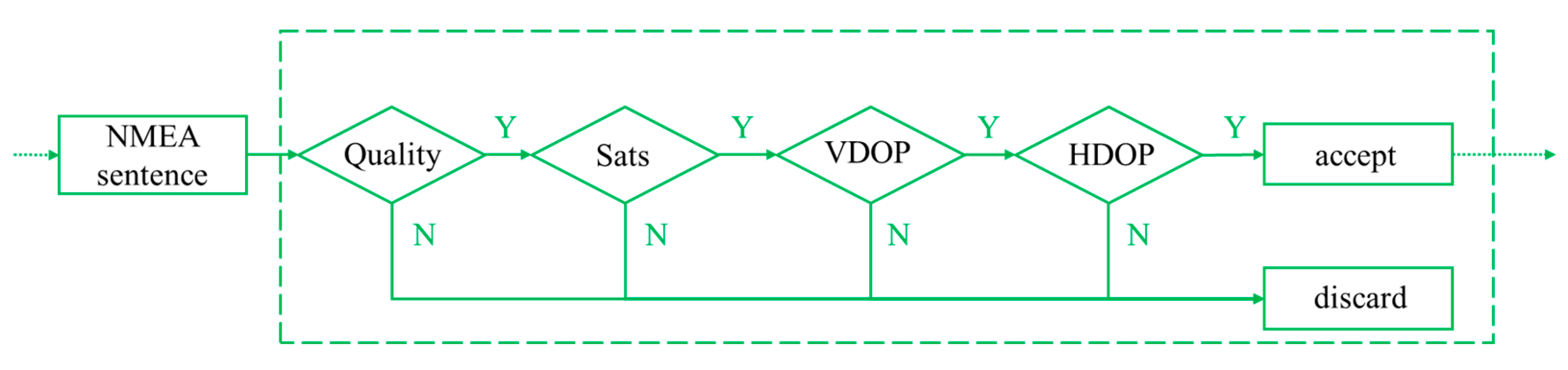
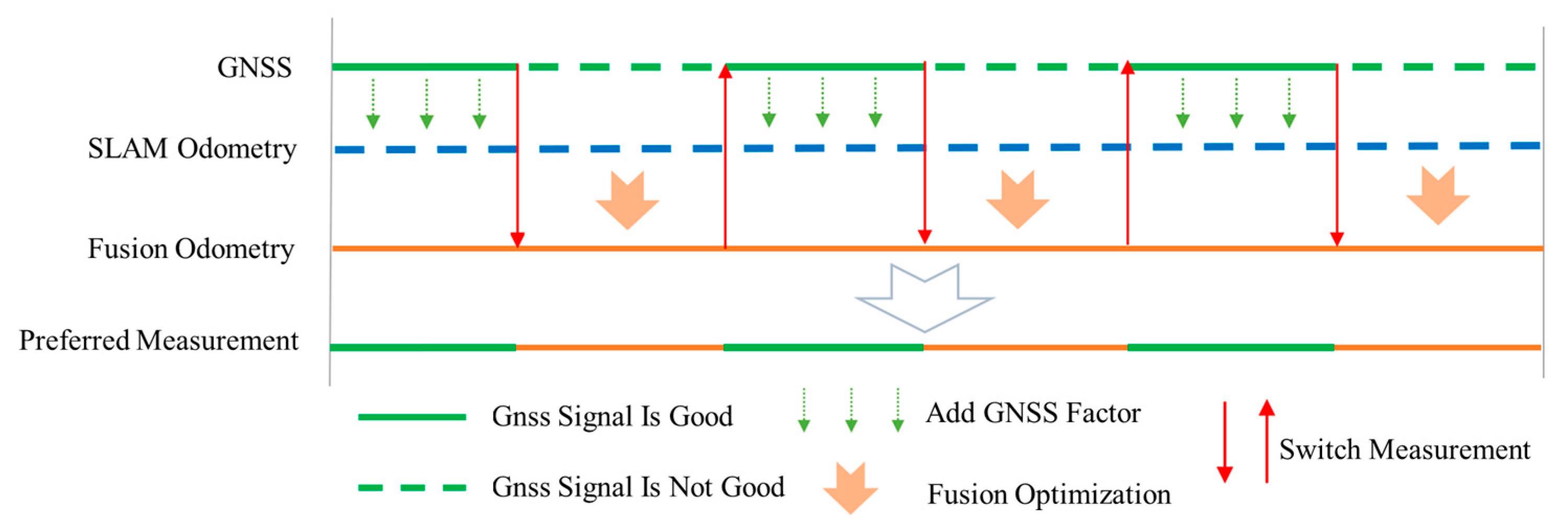
3.2.2. Scene Optimizer (SO)

In most urban scenarios, GNSS and LIO are highly complementary in terms of a working environment. The areas with strong GNSS signals and good satellite geometric distribution usually have relatively few environmental characteristics. The areas with rich environmental characteristics often have high spatial complexity, high buildings, and more trees. The GNSS status in such areas is not good, but the LIO work is stable and the error is small. Therefore, one of the key issues is to strictly monitor and determine the current working state of GNSS. Based on the current main GNSS quality indicators, the Position Dilution of Precision (PDOP), Horizontal Dilution of Precision (HDOP), Vertical Dilution of Precision (VDOP), satellite number SATs, and positioning state quality are selected as the evaluation indicators of GNSS quality. This article obtains GNSS quality indicators from the NMEA (communication protocol standards developed by the National Marine Electronics Association) message of GNSS. Based on the quality evaluation index, this paper constructs the GNSS filter, as shown in Figure 4.
IMU bias drift is usually very accurate under the good constraints of other sensors. The classic GNSS/IMU filtering algorithm establishes a motion model based on IMU, which is used as a predictor. GNSS is regarded as the high-precision observation data and used as an update amount. Centimeter-level positioning can be achieved in a good signal environment. In weak GNSS environments, referring to this structure, the update amount is replaced by the output result of graph optimization so as to achieve higher accuracy than using filtering alone and a higher output frequency than using graph optimization alone. However, the factor map fusion optimization has the limitation of local optimal and global optimal conflicts, especially in the open unshielded zone, and the fusion optimization result MSFO is not necessarily superior to GNSS positioning. Therefore, it is not necessary to use fusion optimization results when GNSS accuracy is reliable. In this paper, the scene is subdivided based on GNSS indicators, and the scene optimizer SO is established. GNSS positioning and MSFO optimized by the factor graph are screened. When GNSS quality is stable, GNSS positioning results are preferred, as shown in Figure 5. It is necessary to note that the optimizer is an optional choice mainly used in post-processing. If it is disabled, the following EKF will be updated completely according to the result of the factor graph.
GNSS and MSFO switching is the key of the scene filter. In the actual scene, the GNSS high-precision working area is distributed in paragraphs due to the specific environmental impact. At the location where the GNSS quality changes, the scene filtering will select the GNSS positioning points ( x g , y g , z g ) and MSFO positioning points ( x m , y m , z m ) at the same time or the nearest time as the switching points, switching between MSFO and GNSS. In actual operation, the carrier re-walks from the non-signal area to the good signal area, the MSFO has been running steadily for a period of time, and a certain error has been accumulated. When the GNSS factor is obtained for error elimination, the MSFO will be adjusted. With the continuous addition of GNSS factors, MSFO will gradually move closer to GNSS. In order to avoid the obvious dislocation of the selected switching time when the gap between the two is too large, it is necessary to delay the switching. When the MSFO is fully adjusted, switching can be realized by adding proximity discrimination.
The discriminant formula is shown in Equation (7).
( x g x m ) 2 + ( y g y m ) 2 + ( z g z m ) 2 < K
where K is the consistency threshold. The smaller the K value is, the smaller the switching point dislocation is, and the whole trajectory is smoother.

3.2.3. EKF Optimization Smoothing

The Scene Optimizer (SO) provides high-quality, low-frequency positioning information, which is further fused with high-frequency IMU information by EKF.
EKF consists of predictions and updates [33]. First, the IMU motion equation is considered, as shown in Equation (8).
x k = f ( x k 1 , v k , w k ) x ˇ k + F k 1 ( x k 1 x ˆ k 1 ) + w k '
where x k is the system state of time k ; f ( x k 1 , v k , w k ) is a nonlinear state transition function; and w k is a process noise, assuming it follows a normal distribution. The right-hand form can be obtained by linearizing the updated estimate x ˆ k 1 at the previous time as a reference point, and F k 1 is the Jacobian matrix of the motion equation. In this paper, 12-dimensional state vector x k = [ p , q , v ] is used, including 3-dimensional coordinates p , three-dimensional attitude q , and velocity v in 3 directions.
The first stage of the algorithm is to perform the prediction step, which predicts the current state estimation and error covariance matrix in time, as shown in Equation (9)
{ P ˇ k = F k 1 P ˆ k 1 F k 1 T + Q k ' x ˇ k = f ( x ˆ k 1 , v k , 0 )
where P ˆ k is the estimated error covariance, and Q k ' is the covariance matrix of noise.
Then, consider the observation equation, as shown in Equation (10).
z k = g ( x k , n k ) y ˇ k + G k ( x k x ˇ k ) + n k '
where z k is the measurement value at that time; g is the nonlinear sensor model that maps the state to the measurement space; and n k is the measurement noise of normal distribution. The observation equation can be linearized on the predicted value x ˇ k of the motion equation to obtain another form. G k is the Jacobi matrix of the observation equation. Then, execute the update step, as shown in Equation (11).
{ K k = P ˇ k G k T ( G k P ˇ k G k T + R k ' ) 1 x ˆ k = x ˇ k + K k ( y k g ( x ˇ k , 0 ) ) P ˆ k = ( 1 K k G k ) P ˇ k
EKF plays two important roles in this scheme. Firstly, it can improve the output frequency of the pose. Secondly, the update selected by the optimizer is switched back and forth between the GNSS pose and the LiDAR pose. Although the switching position is selected, there are still differences. EKF can further optimize and smooth these localities.

4. Experiment and Analysis

In order to verify the feasibility of this scheme and analyze the actual performance of this method qualitatively and quantitatively, this paper designs a series of experiments.

4.1. Self-Collection Dataset Experiments

Based on the unmanned vehicle platform introduced in 3.1, we carried out the acquisition of data. Two datasets were collected, which have different scales and different environmental characteristics. These datasets are playground data and campus data, and the relevant information is shown in Table 2.
It should be noted that all experiments were conducted offline using data collected in advance. Specific tests are as follows.

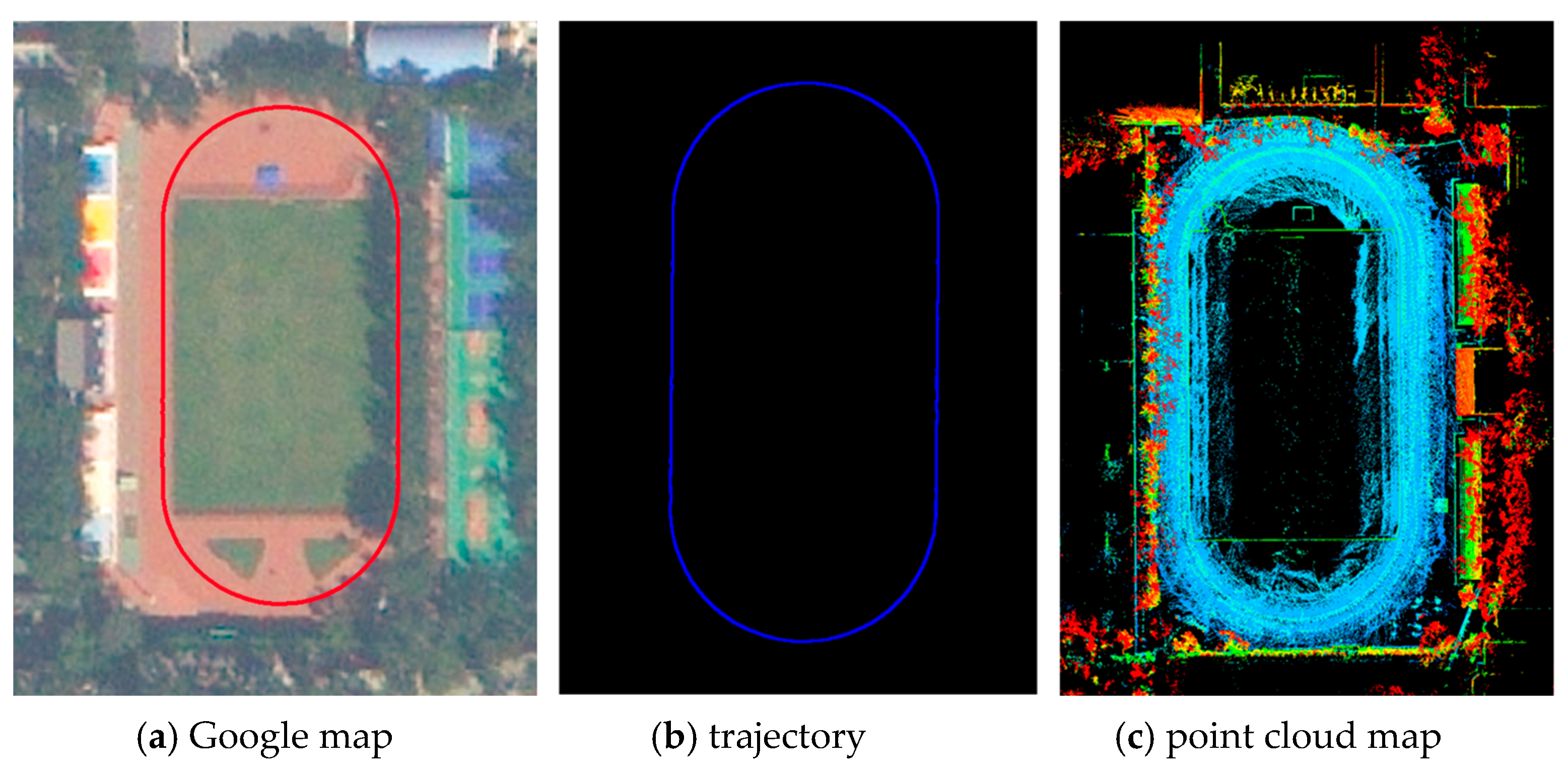
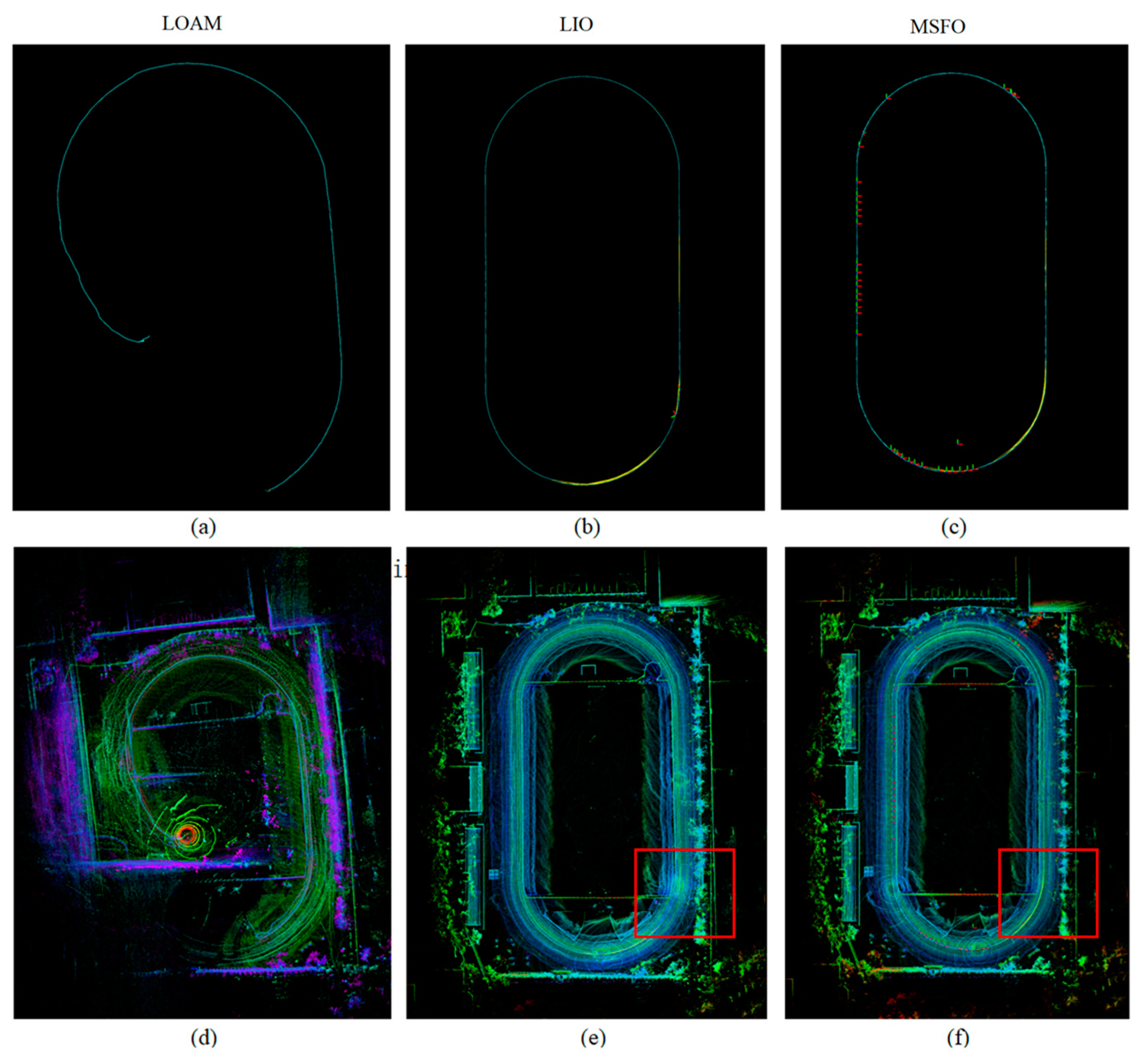
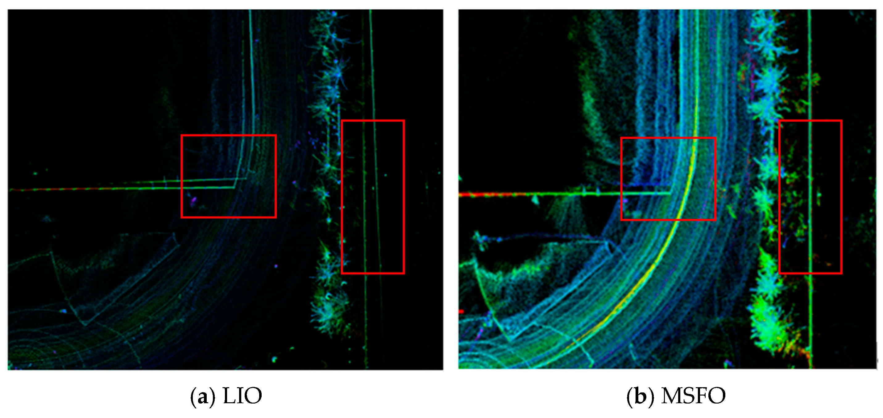
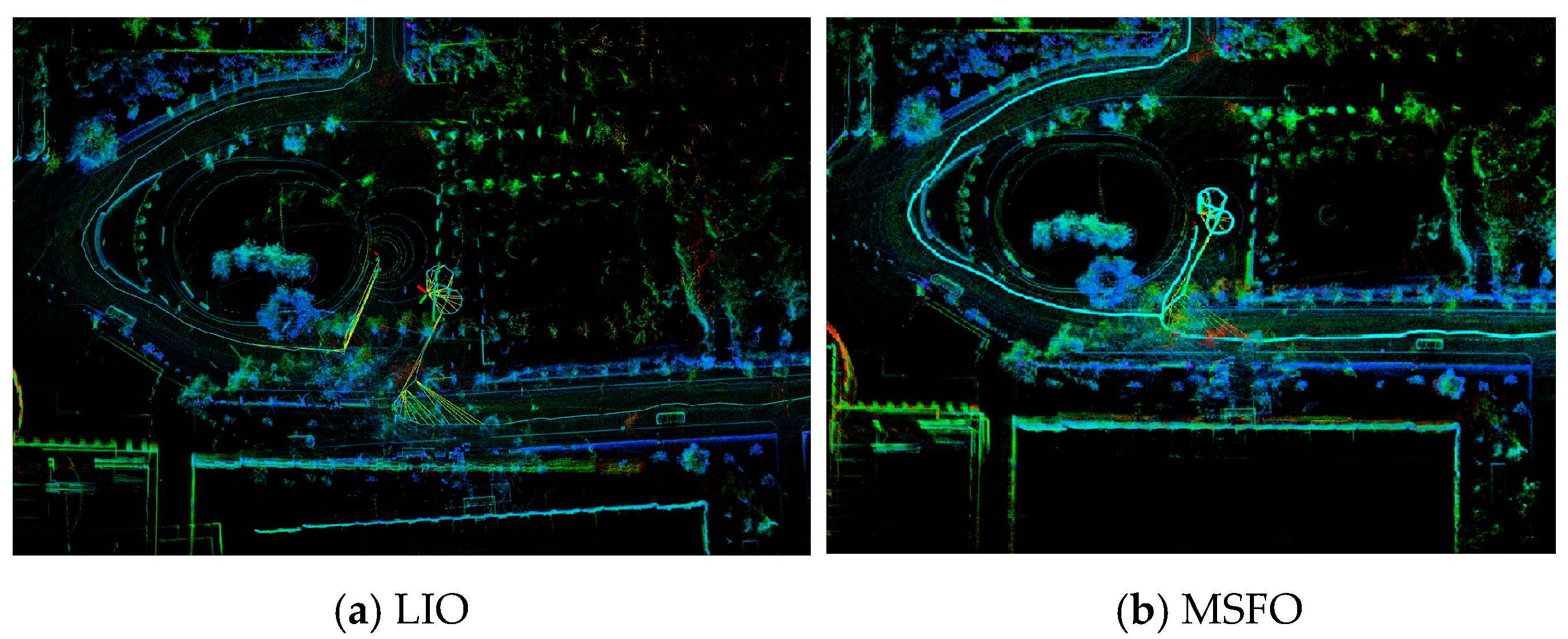
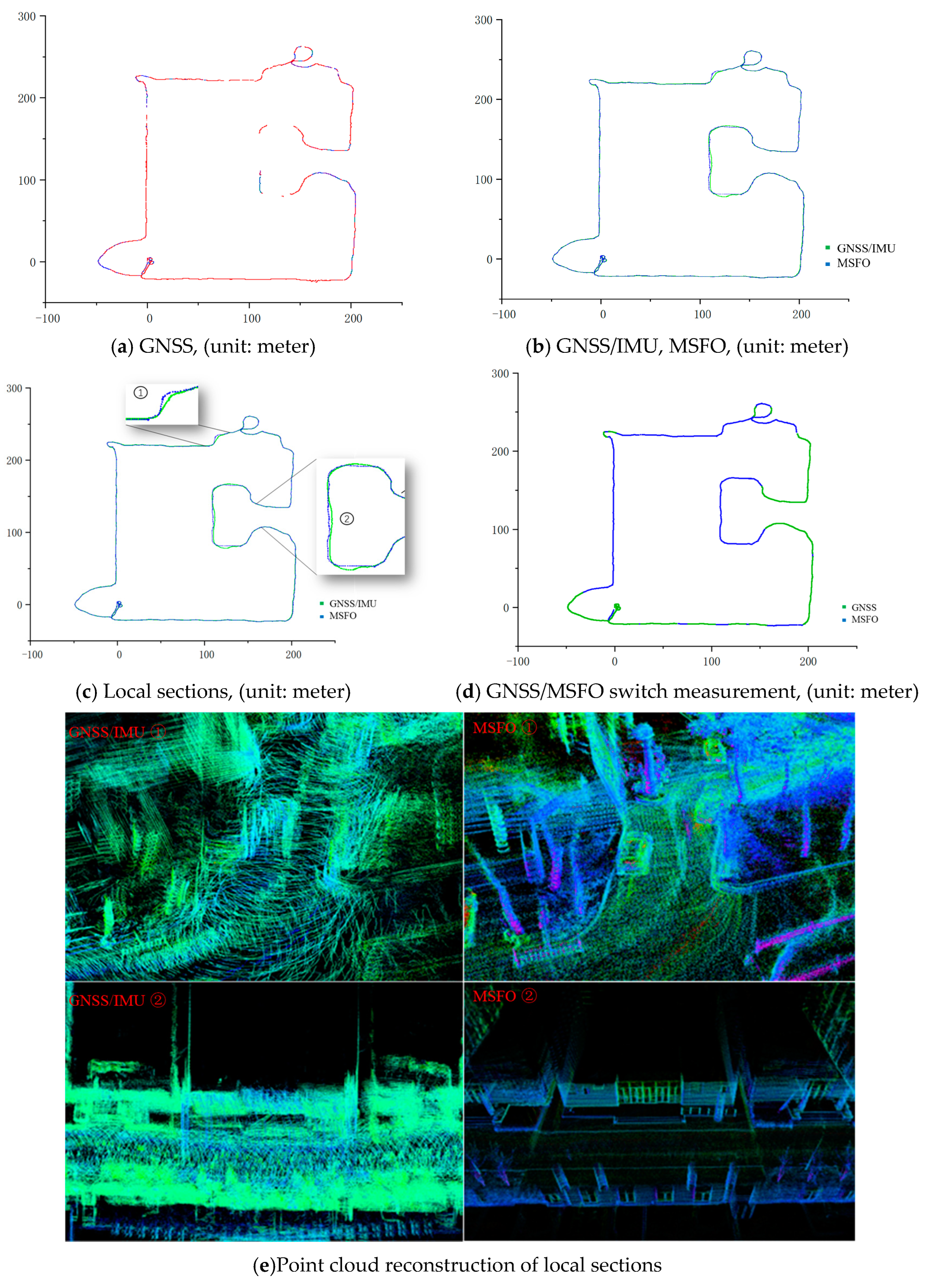
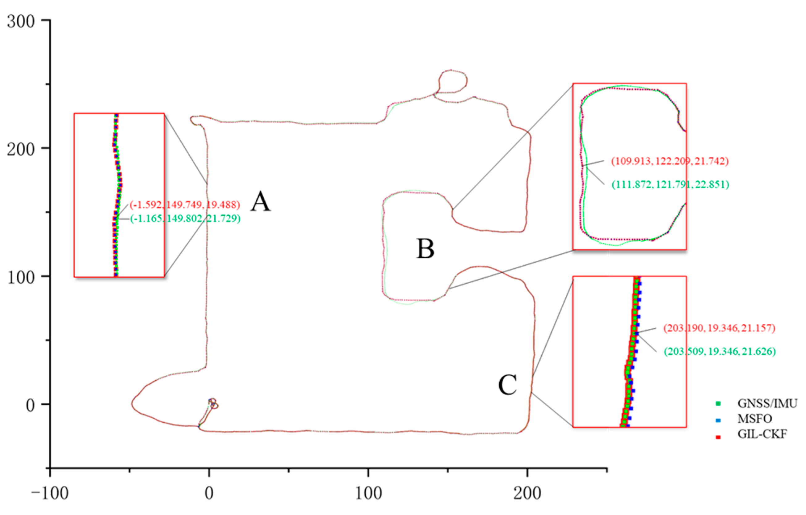
4.1.1. Playground Data
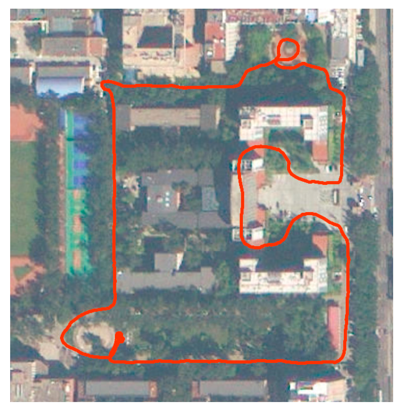
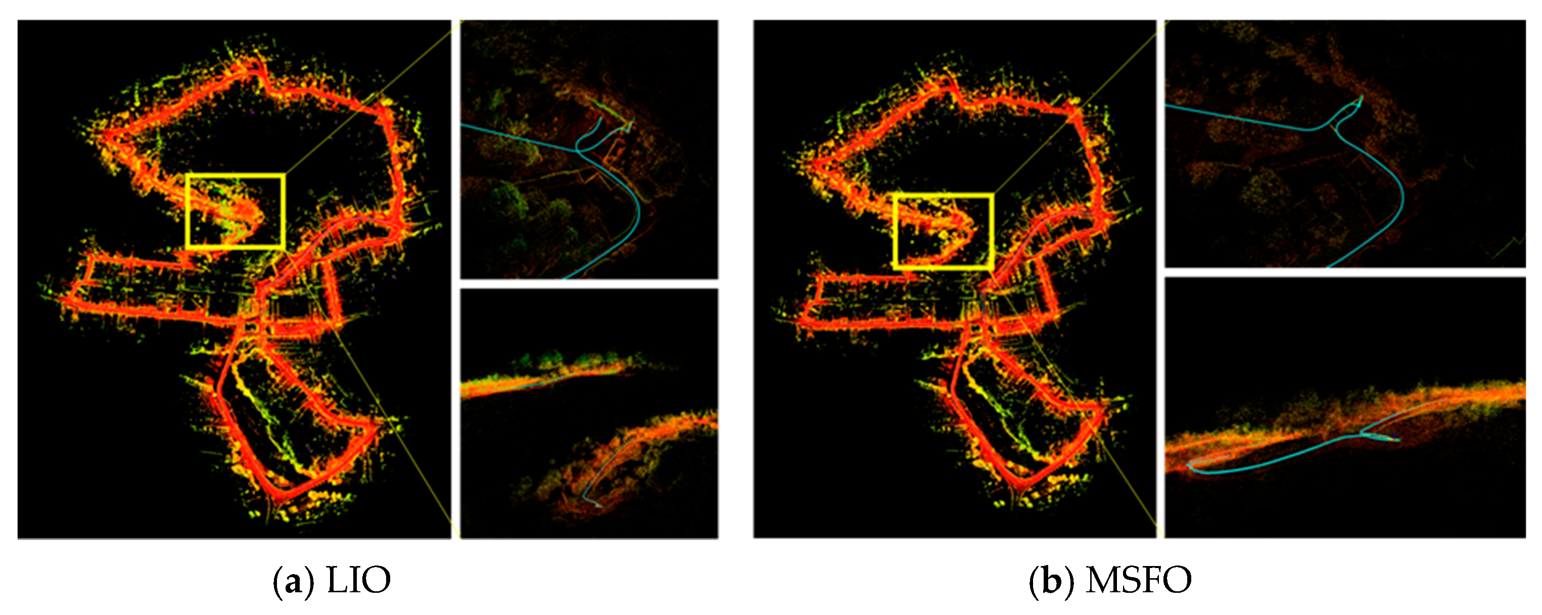
We collected the complete data of the 400 m playground by having the carrier car run along the runway line counterclockwise from the lower right corner. The whole field of view is open, and the number of satellites that can be received is greater than 14, so the GNSS/IMU integrated navigation post-processing results can be regarded as true values. Based on the post-processing software Inertial Explorer, we restored the trajectory of the carrier and established the point cloud, as shown in Figure 6, which are, respectively, the Google map, the carrier trajectory, and the point cloud map corresponding to the playground data.
In order to intuitively show the accuracy of different trajectories, we use these three trajectories and laser raw data for scene reconstruction. The accuracy of the point cloud indirectly reflects the accuracy of the trajectory. Lidar Odometry and Mapping [34] (LOAM), LIO, and MSFO are compared based on the positioning trajectory and mapping performance, as shown in Figure 7.
When the LO algorithm runs to the upper left corner of the playground, there is serious error accumulation and channel degradation. The trajectory recovery is greatly different from the actual situation, as shown in Figure 7a,d. When LIO returns to the original point, an error accumulation of 2.48 m is generated, resulting in point cloud stratification, as shown in Figure 7b,e. After fusing the GNSS factor, the positioning accuracy of MSFO is effectively improved. The error is 0.16 m when returning to the origin, and the point cloud has no obvious stratification, such as Figure 7c,f. The experimental results show that the MSFO system integrated with GNSS can effectively suppress the error accumulation of LIO. The drawings of the partial enlargement of LIO and MSFO are shown in Figure 8.

4.1.2. Campus Data

We collected about 1500 m of data along the campus road. Among them, some areas have a wide field of vision and a good GNSS signal. Some areas are sheltered by tall vegetation and buildings, resulting in a small number of satellites that can be received, and the received GNSS signal was weak. Due to the influence of chassis stability, some sections in the acquisition process have severe jitter and a fast steering bump. The Google map corresponding to the collected campus environment is shown in Figure 9.
Based on the campus dataset, we compared and tested the LOAM, LIO, and MSFO schemes, the factor graph, and the filtering collaborative optimization scheme in this paper. LOAM, LIO, and MSFO are compared based on their positioning trajectories and mapping performances, as shown in Figure 10.
The experimental data show that the LOAM algorithm quickly accumulates the error and runs away, as shown in Figure 10a,d. Although the LIO scheme is superior to LOAM, it also has large cumulative errors, as shown in Figure 10b,c. The overall accuracy of the MSFO scheme is significantly better than the former two, which effectively inhibits the error accumulation of the SLAM system. There is only a ghost phenomenon in the area of intense motion, as shown in Figure 10c,f. The drawings of the partial enlargement of LIO and MSFO are shown in Figure 11.
There is good scene complementarity between GNSS and MSFO, as shown in Figure 12. GNSS loses signals in many road sections and cannot be located, while MSFO can always be located effectively, as shown in Figure 12a,b. Although the GNSS/IMU-based integrated navigation scheme can temporarily provide positioning for the signal occlusion area, the accuracy will decrease, such as in areas 1 and 2 in Figure 12c, which are densely wooded trails and approximately closed corridors. The SO switches measurements between GNSS and SLAM odometry to get the preferred measurement, as shown in (d). Meanwhile, we intercept the point cloud reconstruction of local sections, as shown in (e). In the dense forest section, GNSS/IMU point cloud reconstruction is seen in the upper left corner, and MSFO point cloud reconstruction is seen in the upper right corner; the GNSS/IMU point cloud reconstruction of the closed corridor is seen in the lower left corner, and the MSFO point cloud reconstruction is seen in the lower right corner.
The final pose trajectory of the campus data GIL-CKF is obtained by further fusing the alternating update amounts of GNSS and MSFO (shown in Figure 12) with IMU in EKF, as shown in Figure 13.
In the left part of the figure, because of the serious occlusion of trees and the poor state of the GNSS signal, the SO switches the update amount to MSFO. Select one of the adjacent points to compare (point A), the horizontal difference of 0.427 m, and the elevation difference of 2.241 m. In the middle of the figure on the right is a closed corridor; the GNSS signal is partially lost, and the SO switches to MSFO. Select a pair of adjacent points to compare (point B); the horizontal difference is 1.959 m, and the elevation difference is 1.109 m. In the lower right corner of the figure, the carrier enters the open area. The scene is filtered to determine and switch to a better GNSS track. At the same time, due to the accumulation of errors in the SLAM system, MSFO continues to deviate from GNSS. One pair of adjacent points is selected for comparison (point C). The lateral distance is 0.319 m, and the elevation difference is 0.469 m. This situation is corrected by reaching the middle right. In most open areas, thanks to the high robustness of MSFO, the difference between the GNSS and MSFO trajectories is so small that they appear to fit perfectly.
For the recovery of the carrier motion trajectory, the collaborative optimization scheme of factor graph and filtering proposed in this paper achieves better results than the single GNSS/IMU integrated navigation scheme or the MSFO scheme fused the GNSS using the factor graph. It can not only suppress the error of the SLAM system in the two-step fusion, obtain a relatively more accurate pose in the weak GNSS environment, but also fully retain the high-precision positioning information of GNSS in the signal-free environment, and mitigate the conflict between local optimum and global optimum.

4.2. Utbm Dataset Experiment

In this paper, the open-source urban road dataset Utbm robocar is tested. The dataset collects about 5 km of urban road data from the vehicle [35]. The collection route passes through the city center, parks, residential areas, commercial areas, and bridges and has typical urban characteristics. This paper mainly tests and compares the LIO and MSFO algorithms.
It can be seen in Figure 14 that the MSFO integrated with GNSS can effectively suppress the error accumulation, and it still performs well on large-scale datasets.
In the Utbm dataset test, although GNSS/IMU was able to locate throughout the whole scene range, however, the GNSS/IMU integrated navigation deviated from MSFO in many local areas affected by GNSS signal fading, as seen in Figure 15a. The SO switch measurement between GNSS and MFSO to get the preferred measurement, as shown in Figure 15b.
The accuracy evaluation calculation usually takes differential GNSS positioning as a benchmark, and the output of the algorithm is compared with the absolute accuracy of differential GNSS. However, due to the rapid decline of GNSS positioning accuracy in weak GNSS signal areas, it is not appropriate to still use GNSS as a benchmark. In this paper, the alternating update quantity is used as the benchmark, and GNSS is regarded as the true value in the open signal area to evaluate the accuracy of GIL-CKF and MSFO. In the weak GNSS signal area, MSFO is regarded as the true value, and the accuracy of GIL-CKF and GNSS is evaluated. In this section, 6 points marked in Figure 16 are statistically calculated, and the results are shown in Table 3.
It can be seen from the accuracy statistics that there is a large relative error between GNSS and MSFO at the same time, which usually reaches the meter level. GIL-CKF is close to the selected update amount at the same time, especially the GNSS update section, and the relative error is at the centimeter level, such as points B, D, and E in Table 3. In the MSFO update section, the relative error of GIL-CKF is also maintained at the decimeter level, such as points A, C, and F in Table 3. The relative error of GIL-CKF with different update quantities is different, which is mainly related to the covariance of the two types of update quantities. In open areas, the covariance of GNSS positioning information usually remains at the same level, whereas MSFO has the phenomenon of error accumulation and covariance growth.
At the same time, the cumulative errors of several methods involved in the experiment are also counted. The calculation method of cumulative errors is the distance value between the carrier and the end point coordinates (obtained by post-processing differential GNSS). The results are shown in Table 4.
It can be seen from the cumulative error that the MSFO system integrated with GNSS can effectively suppress the error accumulation of LIO, and the GIL-CKF with alternating updates can further improve the accuracy.

5. Discussion

The pose estimation problem of mobile carriers is the core of mobile measurement. In recent years, with the continuous advancement and exploration of mobile robots and unmanned platforms in various application scenarios, the importance of pose estimation for mobile carriers has become more obvious. At the same time, the diversity of the environment brings great challenges to pose estimation. GNSS signal occlusion, multipath, SLAM scene feature degradation, and dynamic target interference are the difficulties that pose estimation techniques must overcome. This paper argues that multi-sensor fusion is an important way to deal with these challenges. In terms of multi-sensor information fusion, filtering and optimization have their own advantages and disadvantages. The combination of the two will become a consensus, and the combination will become closer. Through the experimental verification of this paper, the technical route of combining graph optimization and filtering fusion can provide a new idea for the current multi-sensor fusion, but there are still some shortcomings that can be further explored, summarized as follows:
(1) The value of the proximity threshold K depends on empirical judgment. Too strict K may lead to the loss of some accurate GNSS positioning information, but too loose may lead to the introduction of some inaccurate GNSS positioning information, thus affecting the accuracy of the results. More effective judgment needs to be considered later;
(2) LIO-SAM is a mature SLAM framework with perfect function and high precision. The implementation of SLAM in this paper draws on LIO-SAM and should be further studied on this basis;
(3) Our scheme is designed under the idea of combining filtering and graph optimization, and this is a loosely coupled design. Graph and filtering are independent of each other, and there is no data exchange between them. It is very fascinating to explore the tight coupling scheme of filtering and graph optimization.

6. Conclusions

Aiming at the demand for high-precision pose estimation in mobile measurement, this paper synthesizes the theoretical results of previous studies, takes the scene complementarity of multi-sensor as the foundation, and adopts the design idea of combining filtering and graph optimization to propose a GNSS/IMU/LiDAR multi-constrained filtering fusion system, GIL-CKF. In this paper, a two-step optimization strategy is adopted. Firstly, factor graph fusion is used to integrate GNSS information into the SLAM system to achieve overall accuracy control. Furthermore, this paper designs a scene optimizer SO based on GNSS quality indicators. With the cooperation of SO, GNSS and MSFO alternately fuse with IMU data in EKF filtering. The experimental equipment of this scheme integrates the Inertial Measurement Unit (IMU), GNSS, and LiDAR. The algorithm makes full use of the high-precision positioning ability of GNSS in the good signal area, the positioning ability of SLAM in the weak GNSS signal area, the error control ability of graph optimization fusion, and the high-frequency positioning ability of filtering to maximize the utilization of limited information.
The experiment with playground data shows that the fusion of high-precision GNSS positioning information and LIO through a factor graph can suppress error accumulation and improve the overall accuracy of SLAM. Experiments based on campus data and Utbm data show that the introduction of scene division based on GNSS quality indicator can retain high-precision positioning information as much as possible, alleviate the conflict between global optimization and local optimization, and improve the pose accuracy of local road sections. SO combined with EKF filtering further optimizes the local trajectory accuracy, and can improve the output frequency and smooth the trajectory. On the whole, the GIL-CKF proposed in this paper achieves better overall trajectory accuracy than a single GNSS/IMU integrated navigation system, or MSFO. It can not only suppress the error of the SLAM system in the two-step fusion to obtain a more accurate pose in the weak GNSS environment but also fully retain the high-precision positioning information of the GNSS in the unblocked environment of the signal to mitigate the conflict between local optimization and global optimization. This scheme is effective in improving pose accuracy and robustness and has the characteristics of full scene coverage, high global accuracy, and high output frequency.

Author Contributions

Conceptualization, R.Z., H.C. and W.W.; methodology, R.Z.; software, H.C. and S.Z.; validation, S.Z., H.C. and C.W.; formal analysis, C.W. and R.Z.; investigation, H.C.; resources, R.Z.; data curation, H.C.; writing—original draft preparation, H.C.; writing—review and editing, H.C. and C.W.; visualization, S.Z.; supervision, R.Z.; project administration, W.W.; funding acquisition, R.Z. All authors have read and agreed to the published version of the manuscript.

Funding

This work was supported in part by the National Natural Science Foundation of China under Grant 42071444 and U22A20568, in part by the National Key Technologies Research and Development Program of China under Grant 2022YFB3904101.

Institutional Review Board Statement

Not applicable.

Informed Consent Statement

Not applicable.

Data Availability Statement

Not applicable.

Conflicts of Interest

The authors declare no conflict of interest.

References

  1. Puente, I.; González-Jorge, H.; Martínez-Sánchez, J.; Arias, P. Review of mobile mapping and surveying technologies. Measurement 2013, 46, 2127–2145. [Google Scholar] [CrossRef]
  2. Han, S.; Wang, J. Integrated GPS/INS navigation system with dual-rate Kalman Filter. GPS Solut. 2012, 16, 389–404. [Google Scholar] [CrossRef]
  3. Boime, G.; Sicsik-Pare, E.; Fischer, J. Differential GNSS+INS for Land Vehicle Autonomous Navigation Qualification. Available online: https://www.gpsworld.com/on-the-road-to-driverless/ (accessed on 1 June 2015).
  4. Han, H.; Wang, J.; Wang, J.; Moraleda, A.H. Reliable Partial Ambiguity Resolution for Single-Frequency GPS/BDS and INS Integration. GPS Solut. 2017, 21, 251–264. [Google Scholar] [CrossRef]
  5. Qian, C.; Liu, H.; Tang, J.; Chen, Y.; Kaartinen, H.; Kukko, A.; Zhu, L.; Liang, X.; Chen, L.; Hyyppä, J. An integrated GNSS/INS/LiDAR-SLAM positioning method for highly accurate forest stem mapping. Remote Sens. 2017, 9, 3. [Google Scholar] [CrossRef] [Green Version]
  6. Dissanayake, M.W.M.G.; Newman, P.; Clark, S.; Durrant-Whyte, H.F.; Csorba, M. A solution to the simultaneous localization and map building (SLAM) problem. IEEE Trans. Robot. Autom. 2001, 17, 229–241. [Google Scholar] [CrossRef] [Green Version]
  7. Bresson, G.; Alsayed, Z.; Yu, L.; Glaser, S. Simultaneous Localization and Mapping: A Survey of Current Trends in Autonomous Driving. IEEE Trans. Intell. Veh. 2017, 2, 194–220. [Google Scholar] [CrossRef] [Green Version]
  8. Cadena, C.; Carlone, L.; Carrillo, H.; Latif, Y.; Scaramuzza, D.; Neira, J.; Reid, I.; Leonard, J.J. Past, Present, and Future of Simultaneous Localization and Mapping: Toward the Robust-Perception Age. IEEE Trans. Robot. 2016, 32, 1309–1332. [Google Scholar] [CrossRef] [Green Version]
  9. Jindal, M.; Jha, A.; Cenkeramaddi, L.R. Bollard Segmentation and Position Estimation from Lidar Point Cloud for Autonomous Mooring. IEEE Trans. Geosci. Remote Sens. 2022, 60, 1–9. [Google Scholar] [CrossRef]
  10. Zhao, P.; Hu, Q.; Wang, S.; Ai, M.; Mao, Q. Panoramic Image and Three-Axis Laser Scanner Integrated Approach for Indoor 3D Mapping. Remote Sens. 2018, 10, 1269. [Google Scholar] [CrossRef] [Green Version]
  11. Gao, Y.; Liu, S.; Atia, M.M.; Noureldin, A. INS/GPS/LiDAR Integrated Navigation System for Urban and Indoor Environments Using Hybrid Scan Matching Algorithm. Sensors 2015, 15, 23286–23302. [Google Scholar] [CrossRef]
  12. Li, D.; Jia, X.; Zhao, J.; Xu, Q.; Zhang, P. An integrated navigation algorithm for SLAM/GNSS/INS based on extended Kalman filter. In Proceedings of the 9th China Satellite Navigation Conference (CSNC), Harbin, China, 23–25 May 2018; pp. 185–189. [Google Scholar]
  13. Rogers, J.G.; Fink, J.R.; Stump, E.A. Mapping with a ground robot in GPS denied and degraded environments. In Proceedings of the 2014 American Control Conference (ACC), Portland, OR, USA, 4–6 June 2014; pp. 1880–1885. [Google Scholar]
  14. Kaess, M.; Johannsson, H.; Roberts, R. Isam2: Incremental Smoothing and Mapping with Fluid Relinearization and Incremental Variable Reordering. In Proceedings of the 2011 IEEE International Conference on Robotics and Automation (ICRA), Shanghai, China, 9–13 May 2011; pp. 3281–3288. [Google Scholar]
  15. Kaess, M.; Ranganathan, A.; Dellaert, F. Isam: Incremental Smoothing and Mapping. IEEE Trans. Robot. 2008, 24, 1365–1378. [Google Scholar] [CrossRef]
  16. Shan, T.; Englot, B.; Meyers, D.; Wang, W.; Ratti, C.; Rus, D. LIO-SAM: Tightly-Coupled Lidar Inertial Odometry via Smoothing and Mapping. In Proceedings of the 2020 IEEE/RSJ International Conference on Intelligent Robots and Systems (IROS), Las Vegas, NV, USA, 24 October–24 January 2021; pp. 5135–5142. [Google Scholar]
  17. Wan, G.; Yang, X.; Cai, R.; Li, H.; Wang, H.; Song, S. Robust and precise vehicle localization based on multi-sensor fusion in diverse city scenes. arXiv 2017, arXiv:1711.05805. [Google Scholar]
  18. Barfoot, T.D. State Estimation for Robotics; Cambridge University Press: Cambridge, UK, 2017; pp. 205–284. [Google Scholar]
  19. Chen, S.; Liu, B.; Feng, C.; Vallespi-Gonzalez, C.; Wellington, C. 3D Point Cloud Processing and Learning for Autonomous Driving: Impacting Map Creation, Localization, and Perception. IEEE Signal Process. Mag. 2021, 38, 68–86. [Google Scholar] [CrossRef]
  20. Wang, Z.; Wu, Y.; Niu, Q. Multi-Sensor Fusion in Automated Driving: A Survey. IEEE Access 2019, 8, 2847–2868. [Google Scholar] [CrossRef]
  21. Fung, M.L.; Chen, M.Z.; Chen, Y.H. Sensor fusion: A review of methods and applications. In Proceedings of the 2017 29th Chinese Control And Decision Conference (CCDC), Chongqing, China, 28–30 May 2017; pp. 3853–3860. [Google Scholar]
  22. Kim, H.; Lee, I. Localization of a car based on multi-sensor fusion. Int. Arch. Photogramm. Remote Sens. Spatial Inf. Sci. 2018, 42, 247–250. [Google Scholar] [CrossRef] [Green Version]
  23. Strasdat, H.; Montiel, J.M.M.; Davison, A.J. Visual SLAM: Why filter? Image Vis. Comput. 2012, 30, 65–77. [Google Scholar] [CrossRef]
  24. Strasdat, H.; Montiel, J.; Davison, A.J. Real-time monocular SLAM: Why filter? In Proceedings of the 2010 IEEE International Conference on Robotics and Automation (ICRA), Anchorage, AK, USA, 3–7 May 2010; pp. 2657–2664. [Google Scholar]
  25. Mourikis, A.I.; Roumeliotis, S.I. A Multi-State Constraint Kalman Filter for Vision-aided Inertial Navigation. In Proceedings of the IEEE International Conference on Robotics and Automation, Roma, Italy, 10–14 April 2007; pp. 3565–3572. [Google Scholar]
  26. Aulinas, J.; Petillot, Y.R.; Salvi, J.; Lladó, X. The slam problem: A survey. CCIA 2008, 184, 363–371. [Google Scholar]
  27. Liang, M.; Min, H.; Luo, R. Graph-based SLAM: A Survey. Robot 2013, 35, 500. [Google Scholar] [CrossRef]
  28. Dellaert, F.; Kaess, M. Factor graphs for robot perception. Found. Trends Robot. 2017, 6, 1–139. [Google Scholar] [CrossRef]
  29. Sola, J. Quaternion kinematics for the error-state Kalman filter. arXiv 2017, arXiv:1711.02508. [Google Scholar]
  30. Trawny, N.; Roumeliotis, S.I. Indirect Kalman filter for 3D attitude estimation. Univ. Minnesota Dept. Comp. Sci. Eng. Tech. Rep. 2005, 2, 2005. [Google Scholar]
  31. Forster, C.; Carlone, L.; Dellaert, F.; Scaramuzza, D. On-manifold preintegration for real-time visual—Inertial odometry. IEEE Trans. Robot. 2016, 33, 1–21. [Google Scholar] [CrossRef]
  32. Forster, C.; Carlone, L.; Dellaert, F.; Scaramuzza, D. IMU Preintegration on Manifold for Efficient Visual-Inertial Maximum-a-Posteriori Estimation. In Proceedings of the Robotics: Science and Systems, Rome, Italy, 13–17 July 2015. [Google Scholar]
  33. Moore, T.; Stouch, D. A Generalized Extended Kalman Filter Implementation for the Robot Operating System. In Proceedings of the 13th International Conference on Intelligent Autonomous Systems (IAS), Padova, Italy, 15–18 July 2016; pp. 335–348. [Google Scholar]
  34. Zhang, J.; Singh, S. LOAM: LiDAR odometry and mapping in real-time. In Proceedings of the Robotics: Science and Systems, Berkeley, CA, USA, 12–16 July 2014. [Google Scholar]
  35. Yan, Z.; Sun, L.; Krajnik, T.; Ruichek, Y. EU Long-term Dataset with Multiple Sensors for Autonomous Driving. In Proceedings of the 2020 IEEE/RSJ International Conference on Intelligent Robots and Systems (IROS), Las Vegas, NV, USA, 25–29 October 2020. [Google Scholar]
Figure 1. The factor graph adopted by our scheme.
Remotesensing 15 00790 g001
Figure 2. Unmanned vehicle hardware platform.
Remotesensing 15 00790 g002
Figure 3. GIL-CKF System Overview. The whole system is divided into three parts: (1) a factor graph fusion system, (2) a measurement update system, and (3) a filtering optimization system. The first part provides low-frequency high-precision fusion information, which is filtered together with GNSS by the second-part scene filtering to provide high-precision measurement for the filter in the third part.
Remotesensing 15 00790 g003
Figure 4. Filter measurement data according to GNSS metrics.
Remotesensing 15 00790 g004
Figure 5. Update amount supply system. SO switch measurement between GNSS and fusion odometry is used to obtain the preferred measurement. The high-quality area of the GNSS signal is distributed in segments due to environmental impact. When the signal is good, it is directly selected as the update amount, and the GNSS factor is added to the SLAM system to form a fusion odometer. When the signal is poor, the fusion odometer is selected as the update amount. The fusion optimization is implemented based on the factor graph fusion system in Figure 3.
Remotesensing 15 00790 g005
Figure 6. Playground experimental data map: (a) the Google map; (b) the trajectory recovered by Inertial Explorer; and (c) the point cloud map reconstructed by (b).
Remotesensing 15 00790 g006
Figure 7. A comparison of LOAM, LIO, and MSFO, respectively, based on the trajectory recovery and mapping reconstruction. The LO trajectory and point cloud reconstruction are very different from the actual situation, and the channel degradation phenomenon occurs, as shown in (a,d). When the LIO returns to the origin, the accumulated error leads to the point cloud separation, as shown in (b,e). After fusing GNSS factors, the positioning accuracy of MSFO is effectively improved and there is no obvious separation of point clouds, as shown in (c,f).
Remotesensing 15 00790 g007
Figure 8. Point cloud details: error accumulation occurs when LIO returns to the origin and leads to point cloud stratification. Meanwhile, this situation does not occur in MSFO.
Remotesensing 15 00790 g008
Figure 9. The Google map and the trajectory of campus experimental data.
Remotesensing 15 00790 g009
Figure 10. A comparison of LOAM, LIO, and MSFO, respectively, based on their trajectory recovery and mapping reconstruction. The LOAM algorithm quickly accumulates errors and fails to chase frames, as shown in (a,d). The accumulated errors of LIO are large, as shown in (b,c). MSFO effectively suppresses the error accumulation of the SLAM system, with ghosting only in some regions, as shown in (e,f).
Remotesensing 15 00790 g010
Figure 11. Point cloud details: error accumulation occurs when LIO returns to the origin and leads to point cloud stratification. Meanwhile, this situation does not occur in MSFO.
Remotesensing 15 00790 g011
Figure 12. GNSS, GNSS/IMU, MSFO, the alternate update amount, and the point cloud reconstruction of local sections. There is good scene complementarity between GNSS and MSFO. The SO switches measurements between GNSS and SLAM odometry to get the preferred measurement, as shown in (d).
Remotesensing 15 00790 g012
Figure 13. The trajectory of the scheme of factor graph and filter collaborative fusion (unit: meter).
Remotesensing 15 00790 g013
Figure 14. A comparison between LIO and MSFO from the point cloud reconstruction: error accumulation occurs when LIO returns to the origin and leads to point cloud stratification. Meanwhile, this situation does not occur in MSFO.
Remotesensing 15 00790 g014
Figure 15. GNSS/IMU, MSFO, and alternate update amount: GNSS/IMU, MSFO, as shown in (a). The SO switch measurement between GNSS and SLAM odometry to get the preferred measurement, as shown in (b).
Remotesensing 15 00790 g015
Figure 16. The trajectory of the complete scheme of the factor graph and filtering cooperation.
Remotesensing 15 00790 g016
Table 1. Parameters of each hardware module.
Hardware ModuleParameters()
NovAtel GNSSDual antenna; measurements (raw) data rate: 20 Hz; nominal accuracy: 1 cm (RTK);
IMUTactical-grade; gyroscopes angular random walk < 0.2 deg/√hr; and accelerometers velocity random walk < 0.035 m/s/√hr.
LiDARNumber of channels: 16; accuracy of ranging: ±3 cm; scanning speed: 5 Hz,10 Hz,20 Hz; horizontal field of view: 360°; and vertical field of view: −15~+15°.
Table 2. Experimental dataset information.
Data NameTrack LengthAcquisition SpeedEnvironmental Conditions
Playgrounds400 m1 m/sUnobstructed
Campus1350 m1 m/sPartially obscured by vegetation, buildings, etc.
Table 3. GNSS/MSFO/GIL-CKF relative accuracy (unit: meter).
MeasurementPointsCoordsGNSSMSFOGIL-CFKGNSS-MSFOGNSS-(GIL-CKF)MFSO-(GIL-CKF)
MSFOAx−345.058−346.122−346.1661.0641.1080.044
y135.007133.756134.1361.2510.871−0.38
z6.71410.59910.341−3.885−3.6270.258
Cx85.70985.13485.1150.5750.5940.019
y−272.204−270.429−270.21−1.775−1.994−0.219
z−48.297−48.025−48.203−0.272−0.0940.178
Fx3.6783.4423.4390.2360.2390.003
y−270.326−271.588−271.1261.2620.8−0.462
z−48.352−48.124−48.24−0.228−0.1120.116
GNSSBx42.49642.15842.4720.3380.024−0.314
y281.017281.219280.832−0.2020.1850.387
z−35.791−36.235−35.810.4440.019−0.425
Dx325.273327.197325.228−1.9240.0451.969
y−484.906−483.345−484.83−1.561−0.0761.485
z−48.351−48.14−48.363−0.2110.0120.223
Ex161.932161.896161.9220.0360.01−0.026
y−663.874−664.2−663.8630.326−0.011−0.337
z−44.548−44.518−44.468−0.03−0.08−0.05
Table 4. Cumulative error (unit: meter).
DatasetsLOLIOMSFOGIL-CKF
Playground dataset>502.480.160.04
Campus dataset>10018.30.380.05
Utbm——>1002.271.36
Disclaimer/Publisher’s Note: The statements, opinions and data contained in all publications are solely those of the individual author(s) and contributor(s) and not of MDPI and/or the editor(s). MDPI and/or the editor(s) disclaim responsibility for any injury to people or property resulting from any ideas, methods, instructions or products referred to in the content.

